Chemometrics-Assisted Calibration of a Handheld LIBS Device for the Quantitative Determination of Major and Minor Elements in Artifacts from the Archaeological Park of Tindari (Italy)

Abstract

In this study, a chemometrics-assisted calibration method was developed for the Z-903 SciAps handheld Laser-Induced Breakdown Spectroscopy (h-LIBS) device. For this purpose, seventeen silica-based standard samples with known chemical composition were collected, pelleted, and analyzed using h-LIBS. Spectral data were pre-processed using a Whittaker filter and normalized via Standard Normal Variate (SNV). The dataset was divided into calibration and validation sets using the Kennard–Stone algorithm. Partial Least Square (PLS) regression was employed for multivariate regression analysis, and a variable selection method (i.e., Variable Importance in Projection, VIP) was applied to reduce the number of predictors. Results from the PLS-VIP approach demonstrated that this device is suitable for the quantitative measurement of nineteen chemical elements, including major and minor elements, achieving significant R² values for major elements including Na (R² = 0.91), Mg (R² = 0.95), and Si (R² = 0.89). The limits of detection reached are satisfying, being, for example, 0.24%, 0.41%, 0.43%, 1.5%, and 1.7% for Na, Al, Ca, Si, and Fe, respectively, among major elements, and 189 ppm, 165 ppm, 203 ppm, and 1 ppm for Ba, Cu, Mn, and Rb, respectively, among minor elements. Uncertainties in prediction of the element concentrations were compared with data from the literature, and the effect of another baseline pretreatment algorithm, airPLS (adaptive iteratively reweighted PLS), was also tested. The method was then applied to nine silica-based artifacts of different typologies sampled from the Archaeological Park of Tindari (Italy), including bricks from the theatre, archaeological glasses, and volcanic rocks.

1. Introduction

Determining the chemical composition of archaeological materials provides essential insights into provenance, manufacturing techniques, and trade routes, as well as supporting the design and development of effective conservation strategies [1,2,3,4,5,6]. Traditionally, such analyses have been conducted in laboratory settings, often requiring the transport of artifacts and, in some cases, the use of invasive or destructive techniques [7]. However, this approach may not be suitable due to the inherent fragility and cultural significance of many archaeological objects, which include natural stones, ceramics, metals, glass, wood, and other organic or inorganic materials [8,9].

Recent advancements in portable instrumentation have allowed for non-destructive or micro-destructive analyses, enabling fast, reliable measurements in situ with minimal impact on the objects, and reducing both sampling risks and costs [10]. Consequently, portable equipment has become essential in the field of Cultural Heritage [11,12,13,14,15,16,17,18]. In this context, Laser-Induced Breakdown Spectroscopy (LIBS) has gained increased attention over the past two decades [19,20,21,22,23,24,25,26,27,28,29,30,31,32,33]. Its appeal in the analysis of Cultural Heritage materials lies in the minimal sample preparation, broad elemental coverage across the periodic table, and flexibility regarding sample geometry or size [34,35,36,37]. Moreover, laser pulses can effectively remove dust coatings, thus facilitating the investigation of weathering layers, either by exposing them directly or through layer-by-layer analysis [38,39].

Despite these advantages, LIBS faces several methodological challenges, most notably the matrix effect, which can cause variability in ablation and emission processes depending on the material. In the context of LIBS applied to archaeological artifacts, the matrix effect refers to the influence exerted by the sample’s chemical composition and physico-structural properties on laser ablation, plasma formation, and spectral emission processes. Variations in the matrix (e.g., silica-based, calcareous), even at constant elemental concentrations, can significantly alter the intensity and shape of spectral lines, thus compromising the accuracy of quantitative analysis. This effect is particularly relevant in archaeological materials, which are often heterogeneous and altered, and requires compensation strategies such as matrix-matched calibration, the use of internal standards, or multivariate data processing (see, e.g., [40,41]). LIBS spectra are also complex, with overlapping emission lines from many elements, making untargeted analysis difficult. Additionally, being a laser-based technique, temperature plays a critical role; the optimal operating range is around 30 °C, which requires careful temperature control during in-situ use.

Thus, while h-LIBS is well-suited for qualitative analysis, achieving accurate quantitative results is more complex. As with other analytical techniques, reliable quantitative LIBS analysis requires proper calibration, typically achieved through calibration curves generated using established standards [42,43,44,45,46,47,48]. Successful quantitative LIBS applications using bench-top instruments have been reported in Cultural Heritage studies [49,50,51,52,53,54]. For instance, Lasheras et al. quantified Fe, Ca, and Mg in archaeological ceramics, using specific calibration standards and selected emission lines [55], while Tankova et al. examined prehistoric bronze artifacts from a Bulgarian site, applying both surface and cross-section analysis to determine Sn and Pb concentrations [56]. However, these studies rely on univariate calibration approaches, which utilize limited spectral information and are more susceptible to fluctuations in plasma conditions.

To overcome these limitations, multivariate calibration methods, particularly those based on chemometrics, are increasingly adopted. For instance, Guan et al. used Double Spectral Correction-Partial Least Squares (DSC-PLS) to determine carbon content in powdered coal with bench-top LIBS [57]. Nardecchia et al. [58] combined LIBS and plasma-induced luminescence hyperspectral imaging using a data fusion strategy to analyze heterogeneous kyanite mineral samples, applying Multivariate Curve Resolution-Alternating Least Squares (MCR-ALS) on compressed datasets to extract chemical features. Dyar et al. [47] employed multivariate regression to analyze geochemical standards obtaining quantitative information about major, minor, and trace elements.

An alternative strategy for quantitative analysis without external calibration is provided by Calibration Free Laser-Induced Breakdown Spectroscopy (CF-LIBS) [59,60,61], which assumes stoichiometric ablation, local thermodynamic equilibrium (LTE), and optically thin plasma. The CF-LIBS approach was used by Senesi et al. [62] in the diagnostic of stone monuments. Despite its theoretical rigor, this method is often complex and case-specific, limiting its widespread application.

Overall, the current literature [37,42,63,64,65] indicates that LIBS for quantitative analysis is still an emerging field, largely limited to a few elements and typically performed with bench-top systems.

Given this context, the aim of this work is twofold: first, to perform a Partial Least Squares-Variable Importance in Prediction (PLS-VIP) chemometrics assisted calibration of the h-LIBS SciAps Z-903 device (see Figure 1), and, secondly, to take advantage of this test to determine the concentration of nineteen elements in silica-based artifacts from the Archaeological Park of Tindari in Sicily, Italy [66,67,68,69,70].

This study is part of a wider research activity at the Archaeological Park of Tindari, conducted both in situ and ex situ, by means of a multi-disciplinary and multi-technique approach, to assess the conservation state of different materials stored in various environments, i.e., a micro-indoor showcase, a warehouse, and outdoor settings, within the framework of the MUR-PNRR Ecosystem SAMOTHRACE (SiciliAn MicronanOTecH Research And innovation CEnter) project.

2. Experimental Section

2.1. Materials and Methods

2.1.1. Standard Samples

To calibrate the h-LIBS device, seventeen silica-based standard samples were selected. These included eight geological certified reference materials (CRMs) and nine geochemical (GEO) samples. The chemical compositions of the CRMs are known and certified, while the GEO samples were quantitatively analyzed at Activation Laboratories using the analytical packages Code 4E and Code 4E-XRF. The Code 4E package involves acid digestion followed by Inductively Coupled Plasma Mass Spectrometry (ICP-MS) analysis for trace elements determination. The Code 4E-XRF package uses lithium tetraborate fusion followed by X-ray fluorescence (XRF) analysis for the quantification of major oxides. Details about CRMs and GEO are provided in Section 3.1.

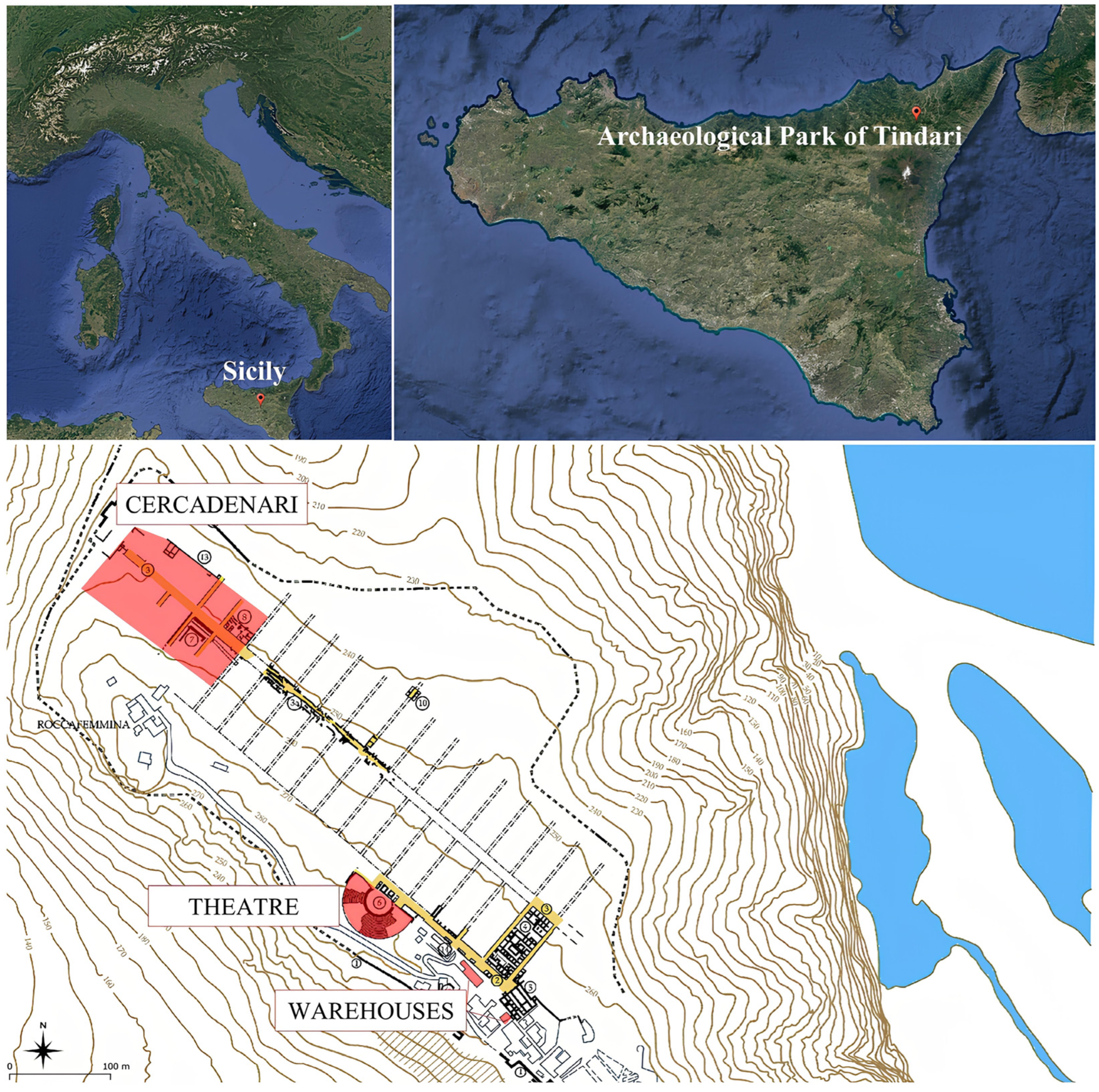
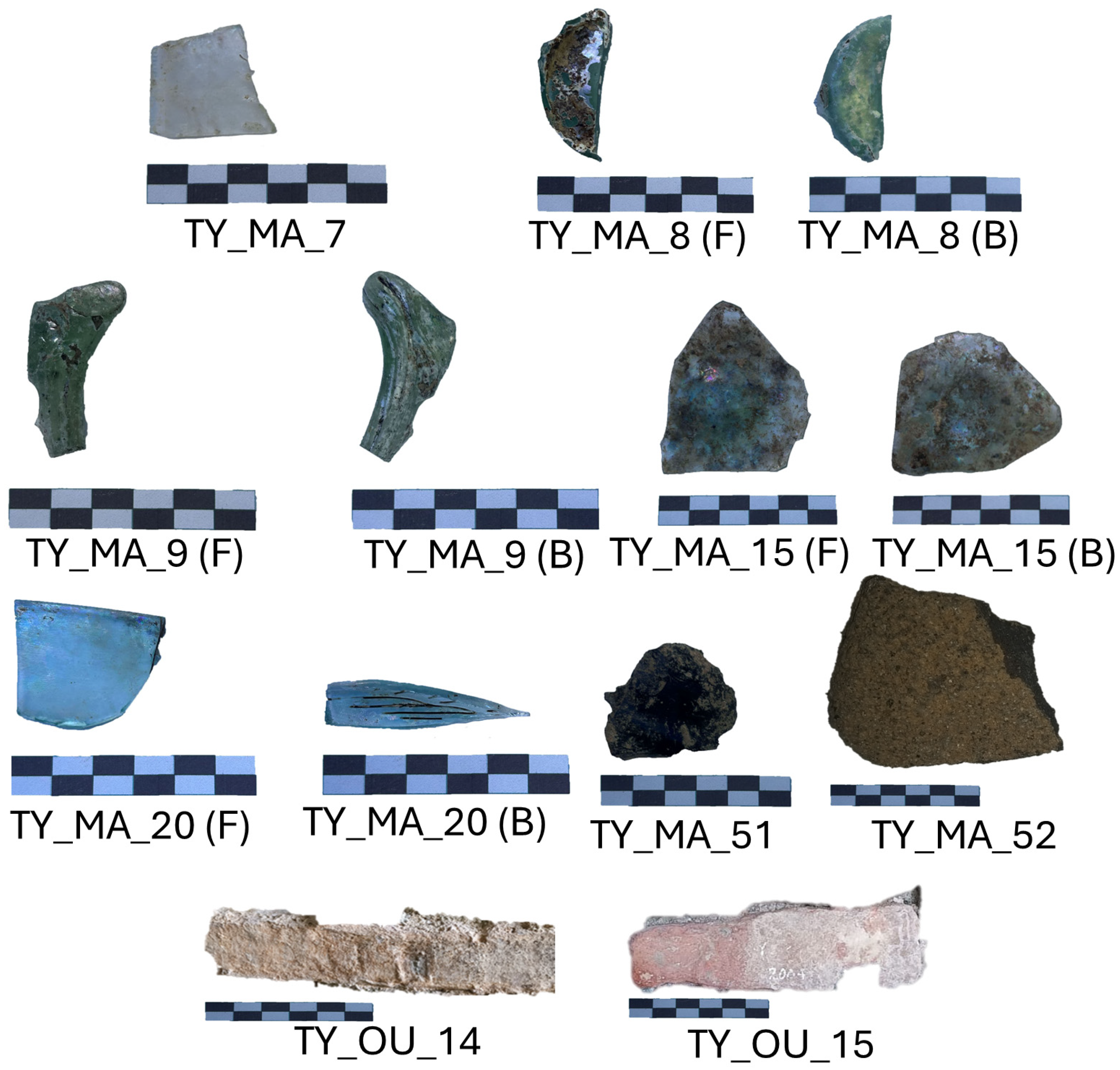
2.1.2. Archaeological Samples

Nine samples were collected from the Archaeological Park of Tindari (Italy) (Figure 2), including two bricks of uncertain age from the theatre, five archaeological glass sherds excavated from the Cercadenari area during various excavation campaigns, a millstone made of volcanic rock, and an obsidian fragment (Figure 3). Specifically, TY_MA_7 is a colorless thin glass fragment, while TY_MA_8 and TY_MA_9 are green glass fragments. These three samples, together with the obsidian fragment (TY_MA_51), were recovered during the August 1970 excavation campaign in the Cercadenari area, specifically from the decumanus, quadrants P19-20–21, layer II. In addition, two further glass fragments were analyzed: TY_MA_15, a base fragment of a glass container discovered in the same area during the July 1993 excavation, and TY_MA_20, a wall fragment of a glass vessel uncovered in the 2023 excavation campaign conducted by the University of Torino (Excavation XVIII-US 667). A fragment of a millstone (TY_MA_52) was sampled from near the main entrance of the Archaeological Park, but no information about the excavation context is available. Finally, TY_OU_14 and TY_OU_15 are bricks located at the central niche in the ring corridor in the theatre orchestra.

Except for the brick fragments and the millstone, all other samples are currently stored in the warehouse of the archaeological park. It is worth mentioning that the sample nomenclature adopted here reflects a broader sampling strategy implemented as part of the aforementioned MUR-PNRR SAMOTHRACE project, which aims to ensure traceability across the extensive dataset generated by the multi-disciplinary investigations currently ongoing on the entire collection of samples.

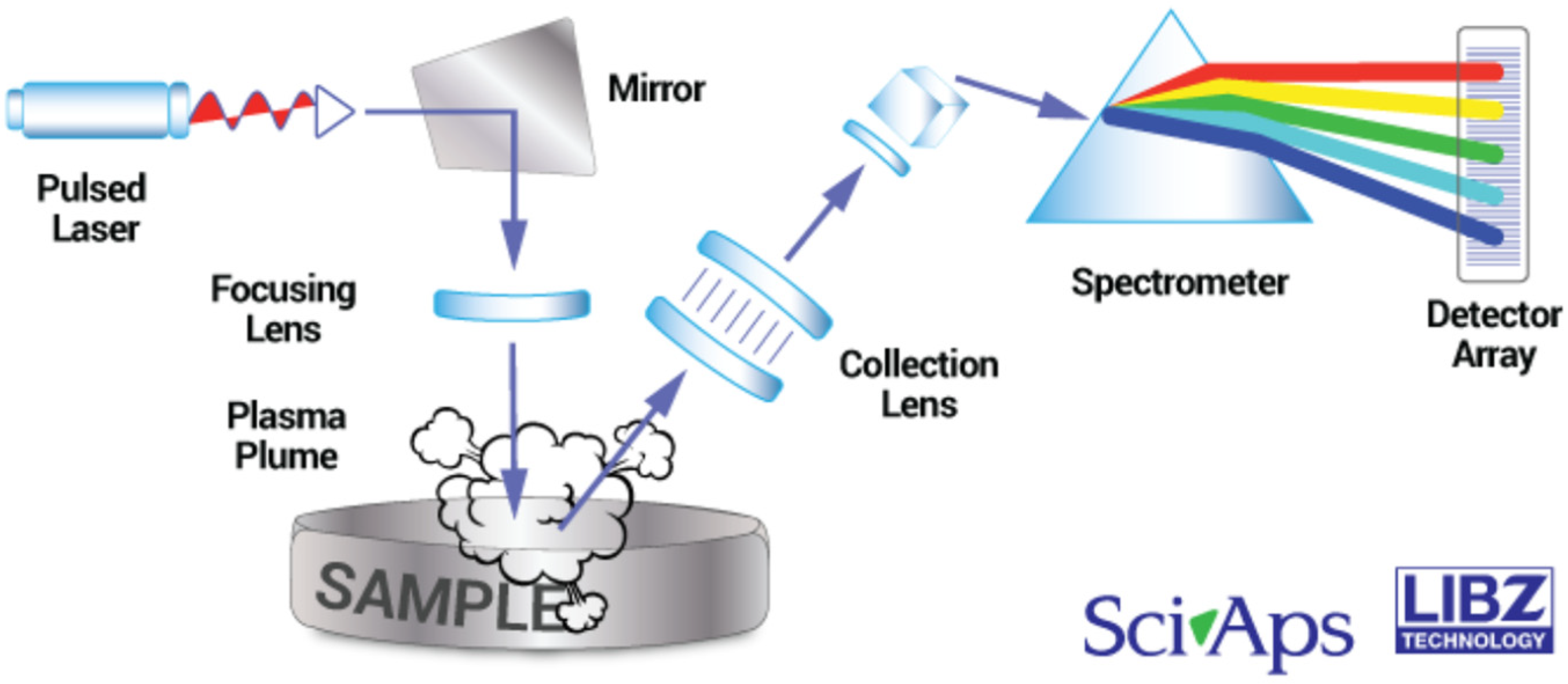
2.1.3. Data Collection with the h-LIBS Device

All standard samples, except NIST612 which is a glass and can be analyzed directly, were in powder form and thus required pressing, using a RETSCH PP 25 press (Dusseldorf, Germany), into pellets prior to being analyzed by h-LIBS (see Supporting Information for further experimental details). Archaeological samples were analyzed in selected areas of the artifacts to minimize problems related to surface roughness or microstructural variations.

Spectral data were collected from both standard and archaeological samples using a Z-903 h-LIBS analyzer (SciAps Inc., Andover, MA, USA) equipped with a 1064 nm Nd:YAg laser covering the 180–950 nm spectral range. In order to enhance the signal-to-noise ratio, spectra were acquired under argon gas (~12 atm) using an argon purge included in the system. For each sample, the LIBS spectrum was obtained, averaging 96 spectral profiles recorded on 6 different locations (16 profiles per location) with a spot size of about 100 μm. The penetration depth was not measured, but the literature reports that it is material-dependent, being around 10 µm for a laser shot [31,38]. If required by the operator, averaging of the spectral profiles was automatically performed by the acquisition software of the equipment. Some random checks were performed to evaluate the repeatability of the spectral profiles. The laser pulsed at a frequency of 1 Hz, and each pulse lasted for 1 ns, delivering 5–6 mJ to the sample. The delay time was 650 ns over a 3 ms integration time. The collected spectra were arranged in a matrix (S_40,23401) with 23,401 variable columns (emissions in arbitrary units as a function of wavelength) and 40 rows. This matrix is composed of two sub-matrices:

• X_17,23401, containing 17 spectra collected from standard samples (i.e., one for each standard sample) for model calibration and validation;
• A_23,23401, consisting of the 23 spectra collected from 9 archaeological samples (being some spectra collected in replicates, see

  Table 1. Number of replicates collected for each investigated archaeological sample.

  Sample Name	Material	Replicates
  TY_MA_7	Colorless glass	1
  TY_MA_8	Green glass	1
  TY_MA_9	Green glass	3
  TY_MA_15	Glass	3
  TY_MA_20	Glass	3
  TY_MA_51	Obsidian	2
  TY_MA_52	Volcanic rock	7
  TY_OU_14	Brick	1
  TY_OU_15	Brick	1

  ) with unknown elemental concentration.

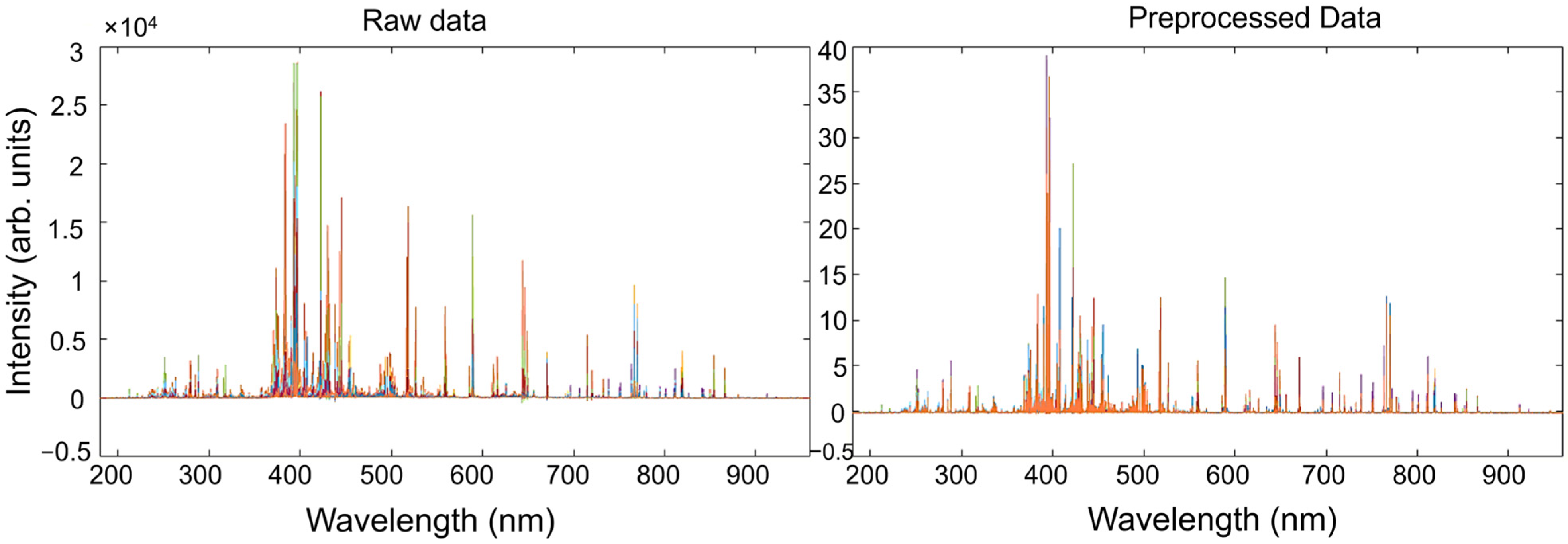
2.1.4. Data Processing

The matrix X, containing the spectra of the standard samples, was pre-processed first with the Weighted Least Squares (WLS) algorithm based on the Whittaker filter (λ = 100, p = 0.001) to establish a baseline, followed by a Standard Normal Variate (SNV) normalization. The adaptive iteratively reweighted Penalized Least Squares (airPLS) algorithm [72] was also tested for the baseline treatment. The matrix containing the concentration of nineteen elements, including major and minor components, in the seventeen standard samples (Y_17,19) was column-wise autoscaled. The instrument was calibrated through the sequential selection of individual elements (i.e., one column vector at a time). The Kennard–Stone algorithm [73] was used to split the X spectral matrix and the Y concentration matrix into calibration (X_cal and Y_cal, 9 samples) and validation (X_val and Y_val, 8 samples) sets. According to Lopez et al. [74], the validation step performed with a subset never used during the calibration and cross-validation steps can be regarded as an external test. However, to enable a more general assessment of the model’s predictive capabilities, another validation step obtained using a strict external test set, namely, a distinct dataset differing not only in composition but also originating from a separate sampling campaign, would be desirable.

The initial calibrated PLS regression model (X_cal vs. Y_cal) was input to a VIP analysis [75]. Since the average of squared VIP scores equals 1, a spectral variable with a VIP score equal or greater than 1 (one) was considered important in the model, whereas variables with VIP scores significantly lower than 1 (one) were excluded from the model. The performance of this step was assessed using the leave-one-out cross-validation approach. The output of the VIP analysis was a reduced spectral matrix (i.e., X_cal’) that was further independently fitted against each Y_cal column vector, corresponding to an element, to build the final PLS-VIP regression model. The optimal number of latent variables for the PLS-VIP analysis was selected by minimizing the Root Mean Squared Error (RMSE) in leave-one-out cross-validation. Then, the model was validated using the X_val and Y_val subsets. After the validation step, the model was applied to the spectral matrix of the archaeological samples (i.e., A) to obtain unknown element concentration, together with the uncertainty associated with the prediction.

In all steps, namely, calibration (cal), cross-validation (CV), and validation (val), the quality of the results was assessed by evaluating the RMSE (see Equation (1)), bias, and correlation coefficient (R², see Equation (2)). The subscripts “cal”, “CV”, and “val” were added to RMSE and R² to define to which phase it refers (e.g., RMSE_cal). The Limit of Detection (LOD) and Limit of Quantification (LOQ) were assessed in the calibration phase by Equations (3) and (4).

$$\mathrm{RMSE}=\sqrt{{\displaystyle \frac{{\sum }_{\mathrm{i}=1}^{\mathrm{N}}{({\mathrm{y}}_{\mathrm{i}}-{\widehat{\mathrm{y}}}_{\mathrm{i}})}^2}{\mathrm{N}}}}$$

(1)

$${\mathrm{R}}^2=1-{\displaystyle \frac{\mathrm{Residual} \mathrm{sum} \mathrm{of} \mathrm{squares}}{\mathrm{Total} \mathrm{sum} \mathrm{of} \mathrm{squares}}}=1-{\displaystyle \frac{{\sum }_{\mathrm{i}=1}^{\mathrm{N}}\left({\mathrm{y}}_{\mathrm{i}}-{ \widehat{\mathrm{y}}}_{\mathrm{i}}\right)}{{\sum }_{\mathrm{i}=1}^{\mathrm{N}}({\mathrm{y}}_{\mathrm{i} }-{\stackrel{-}{\mathrm{y}}}_{\mathrm{i}})}}$$

(2)

$$\mathrm{LOD}={\displaystyle \frac{3·\mathsf{\sigma }}{\mathit{s}}}={\displaystyle \frac{{\mathrm{RMSE}}_{\mathrm{cal}}·\sqrt{{\mathrm{N}}_{\mathrm{cal}}}}{\mathit{s} ·\sqrt{{\mathrm{N}}_{\mathrm{cal}}-1}}}$$

(3)

$$\mathrm{LOQ}=3.3·\mathrm{LOD}$$

(4)

where ${\mathrm{y}}_{\mathrm{i}}$, ${\widehat{\mathrm{y}}}_{\mathrm{i}}$, and ${\stackrel{-}{\mathrm{y}}}_{\mathrm{i}}$ are the ith experimental, calculated from the calibration curve and average concentration, respectively; s is the slope of the predicted vs. measured concentrations values in the calibration phase; and N_cal is the amount of data in the calibration set. The RMSE and bias are expressed in the same unit as the concentration (ppm, in this case), whereas the correlation coefficient is a pure number.

All data pre-processing, variable selection, and regression analysis steps were performed in a Matlab environment version 2023b (The MathWorks Inc., Natick, MA, USA) using PLS toolbox version 8.7.1 (Eigenvector Research, Inc., Manson, WA, USA).

3. Results and Discussion

3.1. Calibration and Validation

Although the number of available standard samples (seventeen) was relatively limited, it was sufficient to calibrate the h-LIBS device. However, not every standard sample contained all elements of the periodic table at concentrations exceeding the declared limit of detection (LOD) [76,77,78]. Consequently, the calibration of the h-LIBS device was performed only for those nineteen elements that surpassed the LOD across all seventeen standard samples.

Selected elements for the CRMs and GEO standard samples, together with their concentrations in parts per million (ppm), are listed in

Table 2. Concentrations (in parts per million, ppm) of the nineteen chemical elements in the certified reference materials (CRMs) and geological samples (GEO) used for the calibration of the h-LIBS device, with some descriptive statistics.

Standard Name	Type	Na	Mg	Al	Si	P	K	Ca	Ti	Mn	Fe	Be	Cu	Zn	Rb	Sr	Y	Mo	Ba	Pb	Ref.
BCR2	CRM	23,148	21,701	71,365	252,479	1569	14,720	50,814	13,567	1522	96,286	2	20	130	46	337	36	251	684	11	a
BIR1A	CRM	13,592	58,423	82,112	223,444	131	241	94,929	5743	1340	79,714	1	121	70	10	109	16	1	7	3	a
GSP2	CRM	20,626	5789	78,882	311,391	1266	44,643	15,000	3953	320	34,263	2	43	120	245	240	28	2	2	42	a
MK1	CRM	24,113	11,276	81,265	299,609	995	33,026	28,071	3097	1239	36,571	4	57	120	160	480	1	3	1400	160	b
NIST612	CRM	97,639	1	12,282	337,434	44	83	86,357	39	77	140	35	34	34	32	10	37	37	36	1	c
GBW07312	CRM	2839	2834	49,235	361,373	235	24,147	8286	1510	1400	34,123	8	1230	498	270	24	29	8	206	285	d
GB07103	CRM	23,223	2533	70,941	340,520	405	41,572	11,071	1720	463	14,964	12	3	28	466	106	62	4	343	31	e
NCSZC71024	CRM	14,765	7778	70,200	312,794	613	22,072	11,929	4310	820	30,907	2	63	100	99	196	23	14	783	182	f
CAL1	GEO	4340	241	39,771	263,087	164	11,249	572	3386	39	420	1	87	37	10	373	4	2	619	10	g
CAL9	GEO	2819	905	45,540	234,473	382	6641	1001	5196	39	17,767	1	36	9	10	841	13	23	1027	16	g
CAL11-BIS	GEO	3042	543	38,925	276,458	458	7513	1644	6299	39	2973	1	24	10	10	856	15	32	1023	23	g
CAL11-ALTO	GEO	964	9410	51,388	245,367	240	2739	4646	3704	287	21,369	1	259	188	10	385	18	3	514	13	g
CAL13	GEO	3005	6575	42,629	248,172	164	6973	4145	3488	62	17,242	1	41	42	10	348	10	11	561	14	g
CAL14-2	GEO	2003	7178	45,117	215,631	262	4151	500	3848	54	42,144	1	16	24	10	437	7	9	641	19	g
CAL15	GEO	1150	11,039	45,910	246,816	175	3155	2859	4124	39	23,013	1	24	34	20	349	13	14	576	8	g
CAL15-SUP	GEO	5564	12,487	46,519	231,434	207	5479	2573	3716	54	28,714	1	27	24	10	364	9	15	562	16	g
CAL16	GEO	2596	1086	44,799	272,905	229	9298	2501	5934	54	5421	1	65	28	30	608	11	11	1100	59	g
m		12,418	9139	52,421	272,380	416	12,284	16,649	4309	413	27,708	4	127	87	74	355	19	23	578	46
s		21,806	12,802	17,910	41,910	403	13,629	28,040	2639	532	24,440	8	271	113	122	227	14	54	369	75
r		97,008	58,423	69,829	145,742	1525	44,560	94,428	13,529	1483	96,147	35	1227	489	466	856	62	251	1399	285
Min		631	1	12,282	215,631	44	83	500	39	39	140	1	3	9	10	10	10	1	2	1
Max		97,639	58,423	82,112	361,373	1569	44,643	94,929	13,567	1522	96,286	35	1230	498	466	856	62	251	1400	285

^a [76]; ^b [77], also known as VS2125-81; ^c [76]; new name is NISTSRM 612; ^d [76]; new name is GSD-12; ^e [76]; new name is GSD-3; ^f [78]; ^g determined in this work.

. A specific portion of this table—comprising the complete set of element concentrations measured in the standard samples—constitutes the previously mentioned Y matrix. Additionally, the table includes descriptive statistical parameters, namely, the mean value (m), standard deviation (s), range (r), minimum value (min.), and maximum value (max.). The elements Na, Mg, Al, Si, K, Ca, and Fe can be regarded as major elements, since their mean concentration (m) is equal or greater than 10,000 ppm (i.e., 1%); P, Ti, Mn, Sr, and Ba can be regarded as minor elements, with an average concentration between 100 and 10,000 ppm, whereas Be, Cu, Zn, Rb, Y, Mo, and Pb are considered as trace elements, since their average concentration is equal to or less than 100 ppm.

Spectral data acquired from the standard samples, allocated in the X matrix, were pre-processed prior to performing multivariate regression vs. the Y concentration matrix. As was previously stated, common issues for LIBS spectra analysis include baseline fluctuations and varying sensitivity among elements. To address these issues, the most commonly adopted approach involves baseline correction and spectral normalization. To this end, a pre-processing step based on the Whittaker filter, followed by a SNV, was carried out. The parameters of the Whittaker filter were chosen to effectively model the baseline while minimizing low-frequency oscillations. A regularization parameter of λ = 100 was selected to impose sufficient smoothness on the estimated baseline without excessively flattening relevant spectral features. The penalty factor p = 0.001 was chosen to allow a degree of sensitivity to subtle baseline variations, improving the separation of weak peaks from the background. This combination enhances the signal-to-noise ratio, particularly for low-intensity spectral lines, which is critical for accurate elemental identification in LIBS analysis. The parameters were initially based on values reported by Nardecchia et al. [58], and subsequently adjusted to optimize performance on the specific dataset used in this work. The impact of such pre-treatments on the LIBS spectra of standard samples, shown in different colors, is illustrated in Figure 4. In parallel, the airPLS algorithm [72] was also tested as an alternative method to the Whittaker filter for baseline correction, offering an adaptive, data-driven approach to suppress background noise while preserving peak integrity. Also, in this case, after baseline correction, the pre-treated spectra were normalized with a SNV transformation. Parameters for the airPLS algorithm were: λ = 10⁵, order of the difference of penalties = 2, Weight of Exception Proportion (WEP) = 0.1, asymmetry p = 0.5, maximum number of iterations = 20. The impact of the use of two different baseline pre-treatments on the calibration and validation performance is discussed later.

The X and Y matrices were split into calibration and validation subsets using the Kennard–Stone algorithm [73], which was chosen because it generates subsets with similar sample density, being a distance-based splitting method. This approach ensures that both subsets maintain a comparable range of element concentration, leading to a more reliable internal validation process.

The calibration phase started with a PLS multivariate regression between the X_cal vs. Y_cal matrices, performed sequentially for each individual element. This approach generated 19 distinct models, one for each element. Subsequently, a VIP analysis was conducted on each PLS model to identify the most correlated variables (i.e., emissions at a specific wavelength) with the column response (i.e., element by element concentration in the Y matrix) using VIP scores [75]. This analysis facilitated variable selection, enabling a refined PLS regression using only the significant variables. The performances of the VIP analysis and the number of Latent Variables (LV) to be retained in the PLS-VIP models were assessed by RMSE_CV.

After this calibration step, the validation step consisted of projecting X_val and Y_val matrices of the standard samples, never used across calibration and cross-validation steps, onto the PLS-VIP models to test its prediction capabilities in terms of element concentration.

A graphical representation of the agreement between predicted and measured concentration of Na, Si, K, and Al is provided in Figure 5. These elements were selected because they are among the major constituents of the standard samples and the corresponding predictive models reflect different performance conditions. Sodium (Na) was included because its model demonstrated the best overall performance, in terms of RMSE and R². Potassium (K) and Silicon (Si) were selected due to their strong performance in the calibration phase, although a decline was observed during validation step. Aluminum (Al), on the other hand, showed satisfactory calibration results, but exhibited a low correlation coefficient in the validation phase.

In each plot, the standard samples used during the calibration phase are represented by grey circles, whereas those employed for validation are depicted as red diamonds. Moreover, the red line represents the regression slope of the predicted vs. measured concentrations during the validation phase, while the green line denotes the ideal 1:1 relationship, indicating perfect accuracy.

Regarding Na, the fitted line (red) and the ideal line (green) are nearly superimposed, revealing excellent predictive capability. Furthermore, reliable predictions are achieved across the entire Na concentration range, as evidenced by the distribution of test samples (i.e., red diamonds) throughout the graph. A similar observation applies to Si, where the fitting line closely follows the ideal one, reflecting satisfying concentration predictions. This indicates the absence of bias (i.e., no systematic deviation from the expected value) during the validation phase. However, in this case, while the samples of validation set cover the full range of Si concentrations, their distribution is skewed towards lower values, with only one validation sample (GB07103) exceeding a Si concentration of 3·10⁵ ppm.

As far as K and Al are concerned, red line and green line are not fully superimposed, indicating the presence of bias. However, if, for K, the validation samples are spread in a manner that traces Si, with more data points at low concentration and one at high concentration (GB07103), in the case of Al validation, the samples are clustered within a narrow concentration range (4 to 7·10⁴ ppm). Such a range corresponds to where the calibration is more reliable but indicates that the model provides less robust concentration estimation for values below 4·10⁴ ppm and above than 7·10⁴ ppm.

The diagrams reporting predicted vs. measured concentration for all elements are given as Supporting Information together with the variables selected (i.e., emission wavelengths) through VIP analysis.

In

Table 3. Summary of the results obtained for the calibration (cal), cross-validation (CV), and validation (val) phases of the PLS-VIP model. Correlation coefficients greater than 0.8 are reported in bold.

			cal			CV			val
Element	Number of Selected Variables	n. LV a	RMSEcal	Bias	R2cal	RMSECV	Bias	R2CV	RMSEval	Bias	R2val	LOD
Na	196	2	2270	0	0.91	2630	−24	0.88	2314	870	0.95	2427
Mg	87	5	3925	−82	0.95	16,807	−5000	0.25	6581	−2583	0.90	4196
Al	180	3	3852	11	0.97	43,307	7771	0.04	16,112	2062	0.01	4118
Si	3893	3	14,261	−110	0.89	22,349	−2465	0.73	29,520	−1545	0.69	15,246
P	1406	4	207	−8	0.81	475	−46	0.18	289	135	0.47	221
K	616	3	6145	15	0.83	13,842	3783	0.21	6072	2747	0.79	6569
Ca	106	3	4034	−309	0.99	13,730	−1875	0.84	3296	−259	0.67	4313
Ti b	356	2	1115	−10	0.67	1566	−3	0.38	801	303	0.63	1192
Mn	30	6	190	0.1	0.89	871	−206	0.01	307	199	0.02	203
Fe	622	3	15,902	−182	0.72	46,406	−10,000	0.20	14,742	8350	0.73	17,000
Be	21,584	2	6	0	0.67	13	−2	0.07	7	−7	0.63	6
Cu	266	3	154	−4	0.53	423	−87	0.05	465	300	0.63	165
Zn	3739	6	14	0	0.99	116	−11	0.32	306	256	0.18	15
Rb	445	5	1.4	0	0.99	32	2	0.90	68	−9	0.96	1
Sr	12,871	6	11	0	0.99	200	−0.37	0.39	134	19	0.60	12
Y c	22	4	2.4	0	0.95	7	−1	0.62	8.9	3.9	0.43	3
Mo	3893	6	10	0	0.98	90	−27	0.01	110	−51	0.05	11
Ba	21	4	177	8	0.86	246	−21	0.75	503	−287	0.01	189
Pb	328	5	39	0	0.84	125	−7	0.05	106	51	0.02	42

^a number of Latent Variables retained; ^b BCR2 CRM was eliminated, ^c GB07103 CRM was eliminated.

, the quality parameters for each individual PLS-VIP model, corresponding to a different element, are reported. Specifically, the table provides RMSE, bias, and R² for each step of the multivariate regression (i.e., calibration, cross-validation, validation), as well as the number of variables selected after the VIP analysis, the number of retained latent variables (LV), and the limit of detection (LOD).

As for the calibration step, the bias is close to zero in all cases, and the correlation coefficients are generally high (>0.8, reported in bold), particularly for the major elements (Na: 0.91; Mg: 0.95, Al: 0.97; Si: 0.89; Ca: 0.99). However, some elements exhibit correlation coefficients in calibration lower than 0.7, including Be (R² = 0.67), Cu (R² = 0.53), and Ti (R² = 0.67), for which a standard sample (BCR2) was determined to be an outlier. For Y, the calibration phase resulted quite satisfactory (R²_cal = 0.95), although one standard sample (GB07103) was excluded.

In the validation step, the quality parameters indicate that the models obtained for Na, Mg, and Rb, are featured by the highest R²_val values, being 0.95, 0.90, and 0.96, respectively.

Overall, it can be inferred that among the major elements, the predictive capabilities of the models are highly satisfactory for both the calibration and validation steps for Na, Ca, Fe, K, Mg, and Si. However, the validation performance for Al could be improved by including additional samples that cover the entire concentration range (see Figure 5 and the low correlation coefficient in Table 3).

For the minor elements (i.e., P, Ti, Mn, Sr, and Ba), the results are generally satisfactory in the calibration phase, whereas the validation phase shows less consistent performance. Notably, Ti and Sr achieved relatively high correlation coefficients (R²_val = 0.63 and 0.60, respectively), and the performance for P (R²_val = 0.47) can be considered moderately acceptable. In contrast, Mn exhibited a low correlation coefficient (R²_val = 0.02), which can be attributed to the clustering of validation samples within a narrow region at low concentration (see Supporting Information), similar to what was observed for Al.

For trace elements, the correlation coefficient is excellent for Rb (R²_val = 0.96) and reasonably satisfactory for Be (R²_val = 0.63), Cu (R²_val = 0.63), and Y (R²_val = 0.43). Conversely, poor correlation was found for Zn (R²_val = 0.18), Mo (R²_val = 0.05), and Pb (R²_val = 0.02). As was observed in the case of Al above, low R²_val values featured by the models obtained for these elements can be interpreted considering the tight concentration range in which the validation samples fall. In the case of Pb, validation samples comprised between 20 and 60 ppm, which is a much narrower range compared to that of the calibration samples (i.e., 1–300 ppm). However, a comprehensive assessment of the predictive capabilities requires considering all quality parameters, as the evaluation of the correlation coefficient alone does not always provide the complete picture. For example, despite the relatively high correlation coefficient for Be (R²_val = 0.63) in the validation phase, the PLS-VIP model cannot be considered fully validated because only two samples in the validation set exhibited concentrations significantly above 1 ppm. As a general result, the models obtained for trace elements must be regarded as tentative.

Regarding the number of variables selected, it is worth noting that for Be, 92% of the total spectral variables (21,584 out of 23,401) were identified as significant in the PLS model. This is another indication that the spectra obtained from the standard samples poorly correlates with the Be concentration.

The referenced scientific literature on PLS regression models (see, e.g., [79,80]) states that the number of samples in a dataset should be sufficiently large in relation to the number of predictor variables to ensure the stability of the model. Although no specific values have been universally defined (apart from the obvious requirement that the number of samples must exceed the number of predictors), this is a crucial aspect that must be carefully considered. In the case presented in this study, the number of standard samples was seventeen, a statistically meaningful quantity, yet not sufficient to build stable models with an excessive number of predictor variables (i.e., latent variables). In Table 3, the number of latent variables retained in each VIP-PLS model is reported. Based on the analysis of these values, it can be stated that the dataset size was adequate to build stable models in all cases where fewer than six latent variables were retained. For those elements where more than five latent variables were retained (i.e., Mn, Zn, Sr, Mo), the dataset size is just sufficient to consider the model reliable. However, in order to increase model robustness, cross-validation was applied during the calibration step. The models that appeared to be less stable—those including six latent variables—are precisely those developed for trace elements, suggesting that the calibration of the h-LIBS device to quantitatively determine the concentration of trace elements with a sufficient precision level must be performed with more than twenty standard samples. The poor predictive ability obtained for trace elements also depended on this aspect.

The LOD values, estimated during the calibration phase, are consistently below 10,000 ppm (1%), with the exception of Si (15,246 ppm, ~1.5%), which is the most abundant element in the standard samples, and Fe (17,000 ppm, ~1.7%). Notably, the LOD for Fe is relatively high and not fully satisfying.

As was previously mentioned above, two different baseline pre-treatments were tested in combination with a SNV normalization, namely, the Whittaker filter (later indicated as Whittaker+SNV) and airPLS (later airPLS+SNV). A numerical comparison of the fitting results, in terms of RMSE and R², both in the calibration and validation phases, is provided in

Table 4. Comparison of quality parameters (RMSE and R²) for the calibration and validation phases using a Whittaker filter followed by a SNV normalization (Wittaker + SNV) and an airPLS algorithm followed by a SNV normalization (airPLS + SNV).

	Whittaker + SNV				airPLS + SNV
Element	RMSEcal	R2cal	RMSEval	R2val	RMSEcal	R2cal	RMSEval	R2val
Na	2270	0.91	2314	0.95	2301	0.90	2554	0.94
Si	14,261	0.89	29,520	0.69	17,087	0.84	26,189	0.85
Al	3852	0.97	16,112	0.01	3700	0.97	16,329	0.19
K	6145	0.83	6072	0.79	3942	0.93	8616	0.69

for the four elements taken as example (i.e., Na, Si, Al, K). Relative diagrams reporting predicted vs. measured concentration are reported as Supporting Information. The comparison indicates that Whittaker+SNV generally provides better performance across the calibration and validation phases. In particular, where the model for Na is concerned, all the parameters considered perform better in the case of Whittaker+SNV (i.e., lower RMSE and higher R²). In the case of Si, the model obtained with a Whittaker+SNV pre-treatment achieved lower RMSE and higher R² values for the calibration phase compared to airPLS, while the contrary is observed for the validation step. A reversed pattern is shown for K and Al, for which airPLS+SNV performed better in the calibration step, while the opposite was observed for the validation step. The selection of the optimal preprocessing strategy appeared to be element-dependent. In general, the Whittaker baseline treatment followed by SNV offers a conservative and stable approach, while airPLS combined with SNV can be beneficial when dealing with more complex or noisy signals, as observed in the case of Si.

The usefulness of soft data-driven models lies in their predictive ability; specifically, in the case of the PLS-VIP approach proposed here, the estimation of the concentration of an element in a sample using h-LIBS. In this context, a critical aspect is the interplay between expected concentration in the sample and the limit of quantification (LOQ). Ideally, the LOQ should be significantly lower than the concentration in the sample, allowing for precise compositional differentiation. On the contrary, when the LOQ exceeds the sample concentration values, the predictions are not sufficiently accurate for practical application.

To provide a clearer understanding of the PLS-VIP model’s applicability, Figure 6 illustrates the LOQ, expressed as a percentage of average and maximum concentration in standard samples, for all the elements studied herein.

For Ca, K, Si, Al, and Na among the major elements, as well as for Ti and Sr among the minor elements and for Rb, Zn, and Y among the trace elements, the LOQ is substantially lower than both the mean and maximum concentrations in the standard samples. This indicates that the model can reliably work when the concentration in a sample is near the mean values of the standard samples (see Table 2). However, for Fe, Mg, and K, despite the model’s good predictive capabilities, the LOQ remains relatively high, making the model practical only when the element concentration exceeds the LOQ. Similar considerations apply to Pb, Cu, Be, Mn, and P. However, in all cases, the LOQ values are well below the maximum element concentration.

From all of the above, despite the relatively limited number of standard samples available in this study, the proposed approach demonstrated satisfactory performance for a significant number of elements, highlighting the effectiveness of PLS-VIP calibration for h-LIBS devices. This outcome is particularly significant, because the calibration of h-LIBS instruments is a difficult, though desirable, task due to the rapidity of the measurements. Moreover, the importance of these finding is further emphasized when one considers that similar calibration strategies reported in the literature are mainly applied to bench-top instruments, often utilizing extensive sets of standard samples [45,46,47,48]. A direct comparison of the uncertainties in prediction determined in this work and those reported in the literature by Dyar et al. [47] is proposed in

Table 5. Comparison of prediction uncertainties obtained in this work and reported in the literature by Dyar et al. [47].

Element	This Work	Dyar et al. [47]
Si	1.5%	1.7%
Ti	0.2%	0.2%
Al	1.2%	0.9%
Fe	2.5%	1.2%
Mg	1.2%	0.7%
Ca	1.0%	0.7%
Na	0.5%	0.4%
K	0.5%	0.6%
P	300 ppm	350 ppm
Ba	450 ppm	232 ppm
Be	9 ppm	0.7 ppm
Cu	400 ppm	26 ppm
Mn	400 ppm	282 ppm
Mo	20 ppm	0.8 ppm
Pb	65 ppm	7 ppm
Rb	50 ppm	52 ppm
Sr	120 ppm	85 ppm
Y	25 ppm	10 ppm
Zn	150 ppm	26 ppm

. The authors published a reference article for the elemental quantification by means of LIBS analysis and trained a PLS model on a multi-matrix dataset containing more than 2000 standard geochemical samples including igneous, sedimentary, and metamorphic rocks. The literature RMSE in prediction, originally reported as oxide percentages, were converted to element percentage to match the concentration scale used in this work.

The uncertain values are highly comparable for all the major elements (i.e., those expressed in%). In particular, the value reported in this work for Si (1.5%) is slightly lower than literature value (1.7%), which is understandable because this work is focused on silica-based materials. Values reported for Ti, Na, and K are not essentially different between the two reports, whereas data listed for Al, Mg, Ca, and Fe are higher than the literature’s values. This latter element, in particular, evidenced some inconsistencies, as the experimental value (2.5%) doubles the literature’s value (1.2%). As minor or trace elements are concerned, uncertainties reported for P, Rb, Sr, and Y are very similar between this work and Dyar et al., who obtained lower RMSE values for the other minor elements, namely, Ba, Be, Cu, Mn, Mo, Pb, and Zn.

3.2. Archaeological Samples

Once the PLS-VIP model was calibrated and validated, it was applied to determine the concentration of 19 elements in the aforementioned archaeological samples (Figure 3) from the Archaeological Park of Tindari. These samples were selected as part of the SAMOTHRACE project, due to their silica-based matrix being compatible with that of the standard samples. The results are presented in

Table 6. Quantitative elemental composition of the samples collected in the Archaeological Park of Tindari.

Element	TY_MA_7	TY_MA_8	TY_MA_9	TY_MA_15	TY_MA_20	TY_MA_51	TY_MA_52	TY_OU_14	TY_OU_15
Na (%)	2.0	2.3	2.3	2.2	2.7	1.0	1.5	1.1	0.9
Mg (%)	<LOQ	<LOQ	<LOQ	<LOQ	1.3	<LOQ	3.6	4.8	6.3
Al (%)	7.6	7.5	6.9	6.5	3.4	3.6	8.8	5.9	5.5
Si (%)	29.4	29.5	29.7	29.8	30.5	30.6	26.2	29.1	30.1
K (%)	<LOQ	<LOQ	<LOQ	0.5	0.8	1.7	1.1	<LOQ	<LOQ
Ca (%)	10.0	10.4	9.8	10.1	8.9	2.4	9.8	10.3	10.8
Ti (%)	<LOQ	<LOQ	<LOQ	<LOQ	<LOQ	<LOQ	<LOQ	<LOQ	0.3
Mn (%)	0.06	0.11	<LOQ	<LOQ	0.09	<LOQ	0.11	0.17	0.47
Fe (%)	<LOQ	<LOQ	<LOQ	5.8	9.8	<LOQ	6.6	8.3	11.5
P (ppm)	<LOQ	<LOQ	<LOQ	<LOQ	<LOQ	<LOQ	<LOQ	<LOQ	<LOQ
Be (ppm)	<LOQ	<LOQ	<LOQ	10	13	19	11	25	29
Cu (ppm)	<LOQ	464	545	<LOQ	<LOQ	<LOQ	<LOQ	<LOQ	<LOQ
Zn (ppm)	<LOQ	<LOQ	<LOQ	<LOQ	<LOQ	153	<LOQ	<LOQ	<LOQ
Rb (ppm)	<LOQ	<LOQ	<LOQ	<LOQ	<LOQ	77	<LOQ	<LOQ	<LOQ
Sr (ppm)	634	610	609	627	708	181	639	724	635
Y (ppm)	<LOQ	<LOQ	31	<LOQ	<LOQ	<LOQ	<LOQ	<LOQ	<LOQ
Mo (ppm)	46	34	63	54	60	<LOQ	43	22	<LOQ
Ba (ppm)	539	<LOQ	<LOQ	527	1622	589	547	513	646
Pb (ppm)	<LOQ	<LOQ	<LOQ	73	104	98	<LOQ	<LOQ	<LOQ

. For samples with multiple replicates, the average concentration values are reported. From a methodological perspective, non-invasive or micro-destructive approaches are preferred when analyzing archaeological materials. In the case of h-LIBS devices, the laser leaves microscopic ablation marks on the sample surface. To minimize any visual or structural impact, measurements were taken on pre-existing fractures or in non-critical areas, following standard archaeometric practices. Visual inspection under magnification confirmed that the laser-induced marks were minimal and did not compromise the integrity or legibility of the artifacts. For fragile or particularly valuable samples, such as some of the glass fragments, measurements were performed on edges or undecorated surfaces to minimize any potential visual impact. When feasible, multiple replicates were collected from different areas of each sample to account for material heterogeneity and improve statistical robustness. However, in certain cases, such as very thin, uneven, or particularly fragile samples, only one representative measurement was acquired. It should be noted that even when a single replicate was reported, this does not correspond to a single laser shot, as already stated in Section 2.1.3. In the case of brick samples, for example, a single acquisition was considered sufficient due to the samples’ uniformity at the analyzed scale. Currently, no comparative data are available to evaluate whether this experimental protocol provides superior performance compared to other analytical techniques (e.g., XRF or ICP-MS).

In detail, the glass samples TY_MA_7 and TY_MA_8 are green glass sherds, while TY_MA_9, TY_MA_15, and TY_MA_20 appear slightly whitish, although they were likely originally transparent. All exhibit a thin, iridescent surface layer indicative of glass degradation [81]. Elemental analysis revealed a primary composition of Si (29–35%), Al (6–8%, except for TY_MA_20), and Ca (9–10%), with consistently low Na (2–3%) and undetectable Ti levels. K remained below 1%. Fe was only detected in TY_MA_15 (5.8%) and TY_MA_20 (9.8%), while Mg and Mn were exclusive to TY_MA_20 (1.3% and 0.1%, respectively). These findings contrast with typical silica-soda-lime Roman glasses, which generally exhibit higher Na contents (ca. 15–17%). The significantly lower Na levels (ca. 2–3%) in these samples are consistent with degradation via alkali leaching, resulting in a hydrated, alkali-depleted surface [6,82,83]. Notably, TY_MA_20 differed from the other samples by showing high levels of Fe, Mn, K, Mg, Pb, and Ba, alongside reduced Al content. Although excavated from the same area as the others, TY_MA_20 was recovered in 2023, about 30 years after the others. This temporal difference, although short from an archaeological perspective, may be relevant due to the Cercadenari area’s agricultural use in recent decades, which may have disturbed the surface and introduced contaminants, particularly K, from fertilizers. The Pb level in TY_MA_20 (104 ppm) may suggest the intentional addition of lead oxide (PbO) as a flux to lower quartz melting temperature [84]: However, the level remains well below the >1% typically found in lead-rich glasses. Another relevant observation is the uniformity of Sr concentrations (ca. 0.1% across all samples, Table 6), supporting the hypothesis of a common sand source, likely coastal sands rich in shell fragments and feldspar impurities (i.e., Al, Ti, Fe, and Mn) [85,86], known for their higher Sr content. Additionally, TY_MA_8 and TY_MA_9, the green glass samples, contain relevant Cu levels (ca. 500 ppm), which likely accounts for their coloration. Overall, the elemental profiles and weathering features are consistent with a silica-soda-lime glass made using natron as a flux and lime as a stabilizer. The results also suggest the use of calcareous sands with feldspar impurities as raw materials [87].

Moreover, the composition of the millstone (TY_MA_52) and obsidian (TY_MA_51) aligns, within experimental errors, with volcanic rocks from Aeolian Islands rather than Mount Etna [88]. This is consistent with the relative geographical proximity of the Aeolian archipelago to the study area.

Concerning the two brick samples, TY_OU_14 is presumed Roman, while TY_OU_15 is believed to be modern. TY_OU_15 exhibits higher Mg and Fe levels and lower Na and Al than TY_OU_14, supporting a distinction in provenance or manufacturing technique. However, conclusive classification requires additional reference samples, including bricks with proven Roman origin. Furthermore, powder X-ray diffraction could help identify high-temperature crystalline phases, potentially distinguishing modern production technologies.

4. Conclusions

In this study, a chemometrics-assisted calibration of a Z-903 h-LIBS device was developed. Spectral data collected on seventeen silica-based standard samples were pre-processed using a Whittaker filter, which performed better than the airPLS algorithm, for baseline correction and normalized via SNV. The Kennard–Stone algorithm was employed to split the dataset into calibration and validation subsets to allow for an internal validation step. Multivariate regression analysis was then carried out by PLS regression, supported by a VIP variable selection routine. The proposed PLS-VIP method proved to be highly promising, achieving limits of quantification (LOQ) comparable with those reported for bench-top LIBS systems. Moreover, the performances in prediction across nineteen elements, encompassing major and minor components, were critically compared to the literature and resulted in satisfactory findings, enabling rapid quantitative determination in situ. However, measurements performed from real artifacts require further optimization to address issues related to surface roughness or microstructural variations, which can affect spectral quality and accuracy.

The calibrated h-LIBS device was then used to analyze nine silica-based samples from the Archaeological Park of Tindari (Italy). The composition of obsidian and millstone fragments suggested a strong similarity to volcanic materials from the nearby Aeolian Islands. For the glass samples, elemental composition revealed consistency with Roman-era glass artifacts found in another Sicilian archaeological area (i.e., Roman Domus of Villa San Pancrazio in Taormina), suggesting a glass-making technology using natron as a flux, lime as stabilizer, and calcareous sands as the primary raw material. The two brick samples exhibited slightly different elemental profiles, potentially indicating varied production techniques. However, definitive classification of these ceramic samples requires additional comparative materials and further analyses, such as powder XRD, to identify specific high-temperature crystalline phases.

While the results highlight the potential of using h-LIBS devices for archaeological materials analysis, the study is limited by the relatively narrow sample diversity, as the calibration was developed using silica-based standards. This restricts the generalizability of the model to other material matrices, such as carbonates or metals. Furthermore, environmental factors such as humidity and temperature fluctuations during measurements were not systematically evaluated, which may influence calibration stability. Another limitation is the absence of a comparative evaluation with other established techniques like pXRF, which is commonly used in the field. Future research will focus on expanding the reference dataset to include a broader range of materials and elemental compositions, including trace and rare-earth elements, to enhance the calibration robustness. This expansion will encompass additional archaeological material typologies, such as mortars, plasters, and alloys from the Tindari site, in alignment with the ongoing SAMOTHRACE project. Furthermore, systematic studies will be conducted to assess the influence of the environmental variables on instrument performance and to benchmark h-LIBS against state-of-the-art techniques like pXRF. Finally, efforts will be made to optimize measurement protocols for real artifact surfaces, addressing surface roughness and microstructural heterogeneity to improve accuracy and reproducibility in situ.

References

1. Rousaki, A.; Moens, L.; Vandenabeele, P. Archaeological Investigations (Archaeometry). Phys. Sci. Rev. 2018, 3, 20170048. [Google Scholar] [CrossRef]
2. Artioli, G. Scientific Methods and Cultural Heritage: An Introduction to the Application of Materials Science to Archaeometry and Conservation Science; Oxford Academic: Oxford, UK, 2010. [Google Scholar]
3. Mazzeo, R. Analytical Chemistry for Cultural Heritage, 1st ed.; Topics in Current Chemistry Collections (TCCC); Springer International Publishing: Cham, Switzerland, 2017; ISBN 978-3-319-52802-1. [Google Scholar]
4. Pollard, A.M.; Heron, C.; Armitage, A.M. Archaeological Chemistry, 3rd ed.; The Royal Society of Chemistry: London, UK, 2016; ISBN 978-1-78262-426-4. [Google Scholar]
5. Pollard, A.M.; Armitage, R.A.; Makarewicz, C.A. Handbook of Archaeological Sciences; John Wiley & Sons Ltd.: Hoboken, NJ, USA, 2023. [Google Scholar]
6. Gomez-Laserna, O.; Irto, A.; Irizar, P.; Lando, G.; Bretti, C.; Martinez-Arkarazo, I.; Campagna, L.; Cardiano, P. Non-Invasive Approach to Investigate the Mineralogy and Production Technology of the Mosaic Tesserae from the Roman Domus of Villa San Pancrazio (Taormina, Italy). Crystals 2021, 11, 1423. [Google Scholar] [CrossRef]
7. Cardiano, P.; Sergi, S.; De Stefano, C.; Ioppolo, S.; Piraino, P. Investigations on Ancient Mortars from the Basilian Monastery of Fragalà. J. Therm. Anal. Calorim. 2008, 91, 477–485. [Google Scholar] [CrossRef]
8. Yogurtcu, B.; Cebi, N.; Koçer, A.T.; Erarslan, A. A Review of Non-Destructive Raman Spectroscopy and Chemometric Techniques in the Analysis of Cultural Heritage. Molecules 2024, 29, 5324. [Google Scholar] [CrossRef]
9. Carter, S.; Clough, R.; Fisher, A.; Gibson, B.; Russell, B.; Waack, J. Atomic Spectrometry Update: Review of Advances in the Analysis of Metals, Chemicals and Materials. J. Anal. At. Spectrom. 2019, 34, 2159–2216. [Google Scholar] [CrossRef]
10. Vandenabeele, P.; Donais, M.K. Mobile Spectroscopic Instrumentation in Archaeometry Research. Appl. Spectrosc. 2016, 70, 27–41. [Google Scholar] [CrossRef]
11. Bardelli, F.; Barone, G.; Crupi, V.; Longo, F.; Majolino, D.; Mazzoleni, P.; Venuti, V. Combined Non-Destructive XRF and SR-XAS Study of Archaeological Artefacts. Anal. Bioanal. Chem. 2011, 399, 3147–3153. [Google Scholar] [CrossRef]
12. Vandenabeele, P.; Edwards, H.G.M.; Jehlička, J. The Role of Mobile Instrumentation in Novel Applications of Raman Spectroscopy: Archaeometry, Geosciences, and Forensics. Chem. Soc. Rev. 2014, 43, 2628. [Google Scholar] [CrossRef]
13. Gómez-Laserna, O.; Arrizabalaga, I.; Prieto-Taboada, N.; Olazabal, M.Á.; Arana, G.; Madariaga, J.M. In Situ DRIFT, Raman, and XRF Implementation in a Multianalytical Methodology to Diagnose the Impact Suffered by Built Heritage in Urban Atmospheres. Anal. Bioanal. Chem. 2015, 407, 5635–5647. [Google Scholar] [CrossRef]
14. Venuti, V.; Fazzari, B.; Crupi, V.; Majolino, D.; Paladini, G.; Morabito, G.; Certo, G.; Lamberto, S.; Giacobbe, L. In Situ Diagnostic Analysis of the XVIII Century Madonna Della Lettera Panel Painting (Messina, Italy). Spectrochim. Acta A 2020, 228, 117822. [Google Scholar] [CrossRef]
15. Spoto, S.E.; Paladini, G.; Caridi, F.; Crupi, V.; D’Amico, S.; Majolino, D.; Venuti, V. Multi-Technique Diagnostic Analysis of Plasters and Mortars from the Church of the Annunciation (Tortorici, Sicily). Materials 2022, 15, 958. [Google Scholar] [CrossRef] [PubMed]
16. Jehlička, J.; Culka, A. Critical Evaluation of Portable Raman Spectrometers: From Rock Outcrops and Planetary Analogs to Cultural Heritage—A Review. Anal. Chim. Acta 2022, 1209, 339027. [Google Scholar] [CrossRef]
17. Briani, F.; Caridi, F.; Ferella, F.; Gueli, A.M.; Marchegiani, F.; Nisi, S.; Paladini, G.; Pecchioni, E.; Politi, G.; Santo, A.P.; et al. Multi-Technique Characterization of Painting Drawings of the Pictorial Cycle at the San Panfilo Church in Tornimparte (AQ). Appl. Sci. 2023, 13, 6492. [Google Scholar] [CrossRef]
18. Frahm, E. Protocols, Pitfalls, and Publishing for pXRF Analyses: From “Know How” to “Best Practices”. J. Archaeol. Sci. 2024, 60, 104831. [Google Scholar] [CrossRef]
19. Harmon, R.S.; DeLucia, F.C.; McManus, C.E.; McMillan, N.J.; Jenkins, T.F.; Walsh, M.E.; Miziolek, A. Laser-Induced Breakdown Spectroscopy—An Emerging Chemical Sensor Technology for Real-Time Field-Portable, Geochemical, Mineralogical, and Environmental Applications. Appl. Geochem. 2006, 21, 730–747. [Google Scholar] [CrossRef]
20. Giakoumaki, A.; Melessanaki, K.; Anglos, D. Laser-Induced Breakdown Spectroscopy (LIBS) in Archaeological Science—Applications and Prospects. Anal. Bioanal. Chem. 2007, 387, 749–760. [Google Scholar] [CrossRef]
21. Fortes, F.J.; Laserna, J.J. The Development of Fieldable Laser-Induced Breakdown Spectrometer: No Limits on the Horizon. Spectrochim. Acta B 2010, 65, 975–990. [Google Scholar] [CrossRef]
22. Botto, A.; Campanella, B.; Legnaioli, S.; Lezzerini, M.; Lorenzetti, G.; Pagnotta, S.; Poggialini, F.; Palleschi, V. Applications of Laser-Induced Breakdown Spectroscopy in Cultural Heritage and Archaeology: A Critical Review. J. Anal. At. Spectrom. 2019, 34, 81–103. [Google Scholar] [CrossRef]
23. García-Escárzaga, A.; Martínez-Minchero, M.; Cobo, A.; Gutiérrez-Zugasti, I.; Arrizabalaga, A.; Roberts, P. Using Mg/Ca Ratios from the Limpet Patella Depressa Pennant, 1777 Measured by Laser-Induced Breakdown Spectroscopy (Libs) to Reconstruct Paleoclimate. Appl. Sci. 2021, 11, 2959. [Google Scholar] [CrossRef]
24. Kuzmanovic, M.; Stancalie, A.; Milovanovic, D.; Staicu, A.; Damjanovic-Vasilic, L.; Rankovic, D.; Savovic, J. Analysis of Lead-Based Archaeological Pottery Glazes by Laser Induced Breakdown Spectroscopy. Opt. Laser Technol. 2021, 134, 106599. [Google Scholar] [CrossRef]
25. Siozos, P.; Hausmann, N.; Holst, M.; Anglos, D. Application of Laser-Induced Breakdown Spectroscopy and Neural Networks on Archaeological Human Bones for the Discrimination of Distinct Individuals. J. Archaeol. Sci. 2021, 35, 102769. [Google Scholar] [CrossRef]
26. Živković, S.; Botto, A.; Campanella, B.; Lezzerini, M.; Momčilović, M.; Pagnotta, S.; Palleschi, V.; Poggialini, F.; Legnaioli, S. Laser-Induced Breakdown Spectroscopy Elemental Mapping of the Construction Material from the Smederevo Fortress (Republic of Serbia). Spectrochim. Acta B 2021, 181, 106219. [Google Scholar] [CrossRef]
27. Richiero, S.; Sandoval, C.; Oberlin, C.; Schmitt, A.; Lefevre, J.-C.; Bensalah-Ledoux, A.; Prigent, D.; Coquidé, C.; Valois, A.; Giletti, F.; et al. Archaeological Mortar Characterization Using Laser-Induced Breakdown Spectroscopy (LIBS) Imaging Microscopy. Appl. Spectrosc. 2022, 76, 978–987. [Google Scholar] [CrossRef]
28. Sun, D.; Zhang, Y.; Yin, Y.; Zhang, Z.; Qian, H.; Wang, Y.; Yu, Z.; Su, B.; Dong, C.; Su, M. A Comparative Study of the Method to Rapid Identification of the Mural Pigments by Combining LIBS-Based Dataset and Machine Learning Methods. Chemosensors 2022, 10, 389. [Google Scholar] [CrossRef]
29. Senesi, G.S.; Allegretta, I.; Marangoni, B.S.; Ribeiro, M.C.S.; Porfido, C.; Terzano, R.; De Pascale, O.; Eramo, G. Geochemical Identification and Classification of Cherts Using Handheld Laser Induced Breakdown Spectroscopy (LIBS) Supported by Supervised Machine Learning Algorithms. Appl. Geochem. 2023, 151, 105625. [Google Scholar] [CrossRef]
30. Harmon, R.S.; Throckmorton, C.S.; Haverstock, G.; Baron, D.; Yohe, R.M.; Hark, R.R.; Knott, J.R. Connecting Obsidian Artifacts with Their Sources Using Multivariate Statistical Analysis of LIBS Spectral Signatures. Minerals 2023, 13, 1284. [Google Scholar] [CrossRef]
31. Mattiello, S.; De Pascale, O.; Palleschi, V.; Fiorentino, G.; Senesi, G.S. Application of Handheld/Portable Spectroscopic Tools to the Identification, Inner Stratigraphy and Mapping of Archaeological Metal Artefacts. J. Phys. Photonics 2024, 6, 035005. [Google Scholar] [CrossRef]
32. Avdeev, G.; Kukeva, R.; Yancheva, D.; Mihailov, V.; Tankova, V.; Dimitrov, M.; Nekhrizov, G.; Stoyanova, R.; Stamboliyska, B. Multi-Analytical Analysis of Decorative Color Plasters from the Thracian Tomb Near Alexandrovo, Bulgaria. Minerals 2024, 14, 374. [Google Scholar] [CrossRef]
33. El-Saeid, R.H.; Abdelhamid, M.; Ali, M.F.; Abdel-Harith, M. LIBS Utilization for the Elemental Analysis of Black Resin and Gold Used by Ancient Egyptians in Embalming. J. Cult. Herit. 2024, 67, 101–110. [Google Scholar] [CrossRef]
34. Cremers, D.A.; Radziemski, L.J. Handbook of Laser-Induced Breakdown Spectroscopy, 1st ed.; John Wiley & Sons Ltd: Chichester, UK, 2006. [Google Scholar]
35. Analytical Methods Committee AMCTB No. 91. Laser-Induced Breakdown Spectroscopy (LIBS) in Cultural Heritage. Anal. Methods 2019, 11, 5833–5836. [Google Scholar] [CrossRef]
36. Anglos, D. Chemical Analysis in Cultural Heritage; Sabbatini, L., van der Werf, I.D., Eds.; De Gruyter: Berlin, Germany, 2020; pp. 77–98. ISBN 978-3-11-045753-7. [Google Scholar]
37. Detalle, V.; Bai, X. The Assets of Laser-Induced Breakdown Spectroscopy (LIBS) for the Future of Heritage Science. Spectrochim. Acta B 2022, 191, 106407. [Google Scholar] [CrossRef]
38. Senesi, G.S.; Carrara, I.; Nicolodelli, G.; Milori, D.M.B.P.; De Pascale, O. Laser Cleaning and Laser-Induced Breakdown Spectroscopy Applied in Removing and Characterizing Black Crusts from Limestones of Castello Svevo, Bari, Italy: A Case Study. Microchem. J. 2016, 124, 296–305. [Google Scholar] [CrossRef]
39. Kechaoglou, E.; Agrafioti, K.A.; Mastrotheodoros, G.P.; Anagnostopoulos, D.F.; Kosmidis, C. On the Study of Paintings’ Stratigraphy by Fs-LIBS and MA-XRF Techniques. J. Anal. At. Spectrom. 2024, 39, 854–867. [Google Scholar] [CrossRef]
40. Donais, M.K.; Douglass, L.; Ramundt, W.H.; Bizzarri, C.; George, D.B. Handheld Laser-Induced Breakdown Spectroscopy for Field Archaeology: Characterization of Roman Wall Mortars and Etruscan Ceramics. Appl. Spectrosc. Pract. 2023, 1, 27551857231175847. [Google Scholar] [CrossRef]
41. Le Guirriec, J.; Alcaina-Mateos, J.; Bousquet, B.; Le Bourdonnec, F.-X.; Sánchez De La Torre, M. Supervised Laser Induced Breakdown Spectroscopy Classification for Prehistoric Chert Provenance: A Methodological Framework. Chemom. Int. Lab. Syst. 2025, 263, 105411. [Google Scholar] [CrossRef]
42. Fu, H.; Jia, J.J.; Wang, H.; Ni, Z.; Dong, F. Calibration Methods of Laser-Induced Breakdown Spectroscopy. In Calibration and Validation of Analytical Methods—A Sampling of Current Approaches; Stauffer, M.T., Ed.; IntechOpen: Rijeka, Croatia, 2018; pp. 87–98. [Google Scholar]
43. Aramendia, J.; Gómez-Nubla, L.; Fdez-Ortiz De Vallejuelo, S.; Castro, K.; Arana, G.; Madariaga, J.M. The Combination of Raman Imaging and LIBS for Quantification of Original and Degradation Materials in Cultural Heritage. J. Raman Spectrosc. 2019, 50, 193–201. [Google Scholar] [CrossRef]
44. Lepore, K.H.; Ytsma, C.R.; Dyar, M.D. Quantitative Prediction Accuracies Derived from Laser-Induced Breakdown Spectra Using Optimized Multivariate Submodels. Spectrochim. Acta B 2022, 191, 106408. [Google Scholar] [CrossRef]
45. Anderson, R.B.; Forni, O.; Cousin, A.; Wiens, R.C.; Clegg, S.M.; Frydenvang, J.; Gabriel, T.S.J.; Ollila, A.; Schröder, S.; Beyssac, O.; et al. Post-Landing Major Element Quantification Using SuperCam Laser Induced Breakdown Spectroscopy. Spectrochim. Acta B 2022, 188, 106347. [Google Scholar] [CrossRef]
46. Lepore, K.H.; Dyar, M.D.; Ytsma, C.R. Sharing Calibration Information among Laser-Induced Breakdown Spectroscopy Instruments Using Spectral Line Binning and Calibration Transfer. Spectrochim. Acta B 2024, 211, 106839. [Google Scholar] [CrossRef]
47. Dyar, M.D.; Ytsma, C.R.; Lepore, K. Geochemistry by Laser-Induced Breakdown Spectroscopy on the Moon: Accuracy, Detection Limits, and Realistic Constraints on Interpretations. Earth Space Sci. 2024, 11, e2024EA003635. [Google Scholar] [CrossRef]
48. Anderson, R.B.; Clegg, S.M.; Frydenvang, J.; Wiens, R.C.; McLennan, S.; Morris, R.V.; Ehlmann, B.; Dyar, M.D. Improved Accuracy in Quantitative Laser-Induced Breakdown Spectroscopy Using Sub-Models. Spectrochim. Acta B 2017, 129, 49–57. [Google Scholar] [CrossRef]
49. Guirado, S.; Fortes, F.J.; Laserna, J.J. Elemental Analysis of Materials in an Underwater Archeological Shipwreck Using a Novel Remote Laser-Induced Breakdown Spectroscopy System. Talanta 2015, 137, 182–188. [Google Scholar] [CrossRef]
50. Agresti, J.; Indelicato, C.; Perotti, M.; Moreschi, R.; Osticioli, I.; Cacciari, I.; Mencaglia, A.A.; Siano, S. Quantitative Compositional Analyses of Calcareous Rocks for Lime Industry Using LIBS. Molecules 2022, 27, 1813. [Google Scholar] [CrossRef]
51. Li, M.; Ruan, F.; Li, R.; Zhou, J.; Zhang, T.; Tang, H.; Li, H. In Situ Simultaneous Quantitative Analysis Multi-Elements of Archaeological Ceramics via Laser-Induced Breakdown Spectroscopy Combined with Machine Learning Strategy. Microchem. J. 2022, 182, 107928. [Google Scholar] [CrossRef]
52. Fabre, C.; Trebus, K.; Tarantola, A.; Cauzid, J.; Motto-Ros, V.; Voudouris, P. Advances on microLIBS and microXRF Mineralogical and Elemental Quantitative Imaging. Spectrochim. Acta B 2022, 194, 106470. [Google Scholar] [CrossRef]
53. Leonidova, A.; Aseev, V.; Prokuratov, D.; Jolshin, D.; Khodasevich, M. Application of Laser-Induced Breakdown Spectroscopy for Quantitative Analysis of the Chemical Composition of Historical Lead Silicate Glasses. Quantum Beam Sci. 2023, 7, 24. [Google Scholar] [CrossRef]
54. Maestro-Guijarro, L.; Sedano, M.; Schibille, N.; Pradell, T.; Castillejo, M.; Oujja, M.; Palomar, T. Determination of Boron Content in Surface Paintings from Historical Stained-Glass Windows. Chem. Methods 2025, 5, e202400057. [Google Scholar] [CrossRef]
55. Lasheras, R.J.; Anzano, J.; Bello-Gálvez, C.; Escudero, M.; Cáceres, J. Quantitative Analysis of Roman Archeological Ceramics by Laser-Induced Breakdown Spectroscopy. Anal. Lett. 2017, 50, 1325–1334. [Google Scholar] [CrossRef]
56. Tankova, V.; Blagoev, K.; Grozeva, M.; Malcheva, G.; Penkova, P. Qualitative and Quantitative Laser-Induced Breakdown Spectroscopy of Bronze Objects. J. Phys. Conf. Ser. 2016, 700, 012003. [Google Scholar] [CrossRef]
57. Guan, C.; Wu, T.; Chen, J.; Li, M. Detection of Carbon Content from Pulverized Coal Using LIBS Coupled with DSC-PLS Method. Chemosensors 2022, 10, 490. [Google Scholar] [CrossRef]
58. Nardecchia, A.; De Juan, A.; Motto-Ros, V.; Gaft, M.; Duponchel, L. Data Fusion of LIBS and PIL Hyperspectral Imaging: Understanding the Luminescence Phenomenon of a Complex Mineral Sample. Anal. Chim. Acta 2022, 1192, 339368. [Google Scholar] [CrossRef]
59. Ciucci, A.; Corsi, M.; Palleschi, V.; Rastelli, S.; Salvetti, A.; Tognoni, E. New Procedure for Quantitative Elemental Analysis by Laser-Induced Plasma Spectroscopy. Appl. Spectrosc. 1999, 53, 960–964. [Google Scholar] [CrossRef]
60. Hu, Z.; Zhang, D.; Wang, W.; Chen, F.; Xu, Y.; Nie, J.; Chu, Y.; Guo, L. A Review of Calibration-Free Laser-Induced Breakdown Spectroscopy. TrAC Trends Anal. Chem. 2022, 152, 116618. [Google Scholar] [CrossRef]
61. John, L.M.; Issac, R.C.; Sankararaman, S.; Anoop, K.K. Multi-Element Saha Boltzmann Plot (MESBP) Coupled Calibration-Free Laser-Induced Breakdown Spectroscopy (CF-LIBS): An Efficient Approach for Quantitative Elemental Analysis. J. Anal. At. Spectrom. 2022, 37, 2451–2460. [Google Scholar] [CrossRef]
62. Senesi, G.S.; Manzini, D.; De Pascale, O. Application of a Laser-Induced Breakdown Spectroscopy Handheld Instrument to the Diagnostic Analysis of Stone Monuments. Appl. Geochem. 2018, 96, 87–91. [Google Scholar] [CrossRef]
63. Senesi, G.S.; Harmon, R.S.; Hark, R.R. Field-Portable and Handheld Laser-Induced Breakdown Spectroscopy: Historical Review, Current Status and Future Prospects. Spectrochim. Acta B 2021, 175, 106013. [Google Scholar] [CrossRef]
64. Limbeck, A.; Brunnbauer, L.; Lohninger, H.; Pořízka, P.; Modlitbová, P.; Kaiser, J.; Janovszky, P.; Kéri, A.; Galbács, G. Methodology and Applications of Elemental Mapping by Laser Induced Breakdown Spectroscopy. Anal. Chim. Acta 2021, 1147, 72–98. [Google Scholar] [CrossRef]
65. Ye, X.; Chen, Y.; Peng, L.; Yang, X.; Bai, Y. Application of Spectroscopy Technique in Cultural Heritage: Systematic Review and Bibliometric Analysis. npj Herit. Sci. 2025, 13, 169. [Google Scholar] [CrossRef]
66. Bernabò Brea, L. Due Secoli Di Studi, Scavi e Restauri Del Teatro Greco Di Tindari. Riv. Dell’istituto Naz. D’archeologia E Stor. Dell’arte 1964/1965, 13–14, 99–144. [Google Scholar]
67. Spigo, U. Tindari. L’area Archeologica e l’antiquarium; Regione Siciliana; Rebus edizioni: Messina, Italy, 2005. [Google Scholar]
68. Leone, R.; Spigo, U. Tyndaris 1. Ricerche Nel Settore Occidentale: Campagne Di Scavo 1993–2004; Regione Siciliana: Palermo, Italy, 2008. [Google Scholar]
69. Astolfi, A.; Bo, E.; Aletta, F.; Shtrepi, L. Measurements of Acoustical Parameters in the Ancient Open-Air Theatre of Tyndaris (Sicily, Italy). Appl. Sci. 2020, 10, 5680. [Google Scholar] [CrossRef]
70. Panagiotonakou, M. Revisiting the Theater of Tyndaris: A New Chronology Proposal. J. Anc. Archit. 2023, 2, 9–30. [Google Scholar]
71. SciAps 2019 LIBS Analyzer Models. Available online: https://www.sciaps.com/libs-handheld-laser-analyzers/z-series/ (accessed on 15 May 2025).
72. Zhang, Z.-M.; Chen, S.; Liang, Y.-Z. Baseline Correction Using Adaptive Iteratively Reweighted Penalized Least Squares. Analyst 2010, 135, 1138. [Google Scholar] [CrossRef] [PubMed]
73. Kennard, R.W.; Stone, L.A. Computer Aided Design of Experiments. Technometrics 1969, 11, 137–148. [Google Scholar] [CrossRef]
74. Lopez, E.; Etxebarria-Elezgarai, J.; Amigo, J.M.; Seifert, A. The Importance of Choosing a Proper Validation Strategy in Predictive Models. A Tutorial with Real Examples. Anal. Chim. Acta 2023, 1275, 341532. [Google Scholar] [CrossRef]
75. Chong, I.-G.; Jun, C.-H. Performance of some Variable Selection Methods When Multicollinearity is Present. Chemom. Int. Lab. Syst. 2005, 78, 103–112. [Google Scholar] [CrossRef]
76. Jochum, K.P.; Nohl, U.; Herwig, K.; Lammel, E.; Stoll, B.; Hofmann, A.W. GeoReM: A New Geochemical Database for Reference Materials and Isotopic Standards. Geostand. Geoanal. Res. 2005, 29, 333–338. [Google Scholar] [CrossRef]
77. Brown, R.H.; Baker, J.; Wilson, W.S. NOAA Technical Memorandum NOS ORCA 94; National Oceanic and Atmospheric Administration: Silver Springs, MD, USA, 1995; p. 480.
78. Labmix24 GmbH Agricultural Soils. NCS ZC71024. Available online: https://labmix24.com/en/products/NCS%20ZC71024 (accessed on 15 March 2025).
79. van der Voet, H. Comparing the Predictive Accuracy of Models Using a Simple Randomization Test. Chemom. Int. Lab. Syst. 1994, 25, 313–323. [Google Scholar] [CrossRef]
80. Wold, S.; Sjöström, M.; Eriksson, L. PLS-Regression: A Basic Tool of Chemometrics. Chemom. Int. Lab. Syst. 2001, 58, 109–130. [Google Scholar] [CrossRef]
81. Silvestri, A.; Molin, G.; Salviulo, G. Archaeological Glass Alteration Products in Marine and Land-Based Environments: Morphological, Chemical and Microtextural Characterization. J. Non-Cryst. Solids 2005, 351, 1338–1349. [Google Scholar] [CrossRef]
82. Palomar, T.; Oujja, M.; García-Heras, M.; Villegas, M.A.; Castillejo, M. Laser Induced Breakdown Spectroscopy for Analysis and Characterization of Degradation Pathologies of Roman Glasses. Spectrochim. Acta B 2013, 87, 114–120. [Google Scholar] [CrossRef]
83. Gueli, A.M.; Pasquale, S.; Tanasi, D.; Hassam, S.; Lemasson, Q.; Moignard, B.; Pacheco, C.; Pichon, L.; Stella, G.; Politi, G. Weathering and Deterioration of Archeological Glasses from Late Roman Sicily. Int. J. Appl. Glass Sci. 2020, 11, 215–225. [Google Scholar] [CrossRef]
84. Ricciardi, P.; Colomban, P.; Tournié, A.; Macchiarola, M.; Ayed, N. A Non-Invasive Study of Roman Age Mosaic Glass Tesserae by Means of Raman Spectroscopy. J. Archaeol. Sci. 2009, 36, 2551–2559. [Google Scholar] [CrossRef]
85. Freestone, I.C.; Leslie, K.A.; Thirlwall, M.; Gorin-Rosen, Y. Strontium Isotopes in the Investigation of Early Glass Production: Byzantine and Early Islamic Glass from the Near East. Archaeometry 2003, 45, 19–32. [Google Scholar] [CrossRef]
86. Degryse, P.; Scott, R.B.; Brems, D.T. The Archaeometry of Ancient Glassmaking: Reconstructing Ancient Technology and the Trade Ofraw Materials. Perspective 2014, 2, 224–238. [Google Scholar] [CrossRef]
87. Silvestri, A. The Coloured Glass of Iulia Felix. J. Archaeol. Sci. 2008, 35, 1489–1501. [Google Scholar] [CrossRef]
88. Peccerillo, A. Plio-Quaternary Volcanism in Italy Petrology, Geochemistry, Geodynamics; Springer: Berlin/Heidelberg, Germany, 2005. [Google Scholar]
Figure 1. Diagram of the SciAps Z-903 h-LIBS device used in this work (credit: SciAps Inc. [71]).
Applsci 15 06929 g001
Figure 2. Map of Italy (top left), location of the Archaeological Park of Tindari in Sicily (Italy) (top right), and detailed map of the Archaeological Park of Tindari (bottom).
Applsci 15 06929 g002
Figure 3. Archaeological samples collected from the Archaeological Park of Tindari (Italy) along with photographic scale. Each colored segment represents 1 cm length × 0.5 cm height, providing a reference for size. (F): front side, (B): back side.
Applsci 15 06929 g003
Figure 4. Effect of the pre-treatments on the LIBS spectra of standard samples along the entire spectral range. Each color represents the spectral profile of a standard sample.
Applsci 15 06929 g004
Figure 5. Plot of predicted (obtained from the PLS-VIP model) vs. measured concentration for Na, Si, K, and Al. Grey circles: standard samples used in the calibration step; red diamonds: standard samples used for validation; red lines: fitting of predicted vs. measured concentrations values during validation; green lines: ideal fitting.
Applsci 15 06929 g005
Figure 6. LOQ (%) of each element as percentages of the mean (blue bar) and maximum (red bar) concentration, for the standard samples.
Applsci 15 06929 g006