A Framework for Low-Carbon Container Multimodal Transport Route Optimization Under Hybrid Uncertainty: Model and Case Study

Abstract

To enhance the operational efficiency of container multimodal transportation and mitigate carbon emissions during freight transit, this study investigates carbon emission-conscious multimodal transportation route optimization models and solution methodologies. Addressing the path optimization challenges under uncertain conditions, triangular fuzzy numbers are employed to characterize transportation time uncertainty, while a scenario-based robust regret model is formulated to address freight price volatility. Concurrently, the temporal value attributes of cargo are incorporated by transforming transportation duration into temporal costs within the model framework. Through the implementation of four distinct low-carbon policies, carbon emissions are either converted into cost metrics or established as constraint parameters, thereby constructing an optimization model with total cost minimization as the objective function. For model resolution, fuzzy chance-constrained programming is adopted for defuzzification processing. Subsequently, a multi-strategy improved whale optimization algorithm (WOA) is developed to solve the formulated model. Numerical case studies are conducted to validate the proposed methodology through comparative analysis with conventional WOA implementations, demonstrating the algorithm’s enhanced computational efficiency. The experimental results confirm the model’s capability to adapt multimodal transportation schedules for cargo with varying temporal value attributes and effectively reduce CO₂ emissions under different carbon reduction policies. This research establishes a comprehensive decision-making framework that provides logistics enterprises with a valuable reference for optimizing low-carbon multimodal transportation operations.

1. Introduction

With the rapid development of modern logistics, where clients increasingly demand time-sensitive and reliable transportation services, the logistics industry faces critical challenges in reducing operational costs, enhancing transportation efficiency, and mitigating carbon emissions [1]. Traditional unimodal transportation systems have become inadequate to meet multifaceted market requirements, while uncertainties in transit time, freight pricing, and transportation demand increasingly compromise service reliability [2,3,4]. Multimodal transportation emerges as an efficient, flexible, and environmentally sustainable collaborative solution that systematically enhances operational efficiency, strengthens service reliability, and significantly reduces carbon emissions through the integrated optimization of multiple transport modes [5]. Addressing uncertainty-induced impacts and formulating adaptive multimodal solutions under diverse scenarios thus represents a pivotal approach to advancing organizational competence and competitive advantage in multimodal operations [6].

Containerized multimodal transport constitutes a complex dynamic system facing numerous challenges characterized by uncertainty, where fluctuations in transportation costs present a persistent difficulty in cargo transactions, primarily stemming from market dynamics—such as fluctuating supply and demand during peak logistics seasons leading to capacity constraints and route congestion, coupled with volatile fuel prices driven by international crude oil markets and geopolitical factors directly impacting unit rates—and disruptive emergencies, including natural disasters or policy adjustments necessitating additional cross-regional transport segments and resulting in multifaceted cost increases that amplify price uncertainty [7]. Beyond cost uncertainty, transport time uncertainty is equally critical, as operations are frequently disrupted by emergencies and unforeseen events like extreme weather, seasonal bottlenecks, equipment failures, and urgent order insertions, impeding adherence to planned schedules [8]. While existing research predominantly addresses either transport time uncertainty or demand uncertainty in isolation, a notable gap persists concerning multimodal transport path optimization under the combined uncertainty of both transportation costs and time, thereby establishing the theoretical significance and practical implications of this paper’s focus.

This paper develops a methodological framework incorporating carbon taxation, carbon trading, mandatory emission limits, and carbon offset mechanisms to regulate emissions while simultaneously addressing uncertainties in cargo arrival times and unit freight pricing. By analyzing the time–value attributes of heterogeneous cargo types. A cost-minimization optimization model for low-carbon multimodal routing is formulated, solved through an improved whale optimization algorithm (IWOA). Parametric sensitivity analysis is conducted to examine cargo-specific routing patterns across scenarios. Government transportation departments or multimodal transport operators may be interested in this study.

The remainder of this study is organized as follows: Section 2 reviews literature on multimodal transportation, low-carbon logistics, and optimization algorithms. Section 3 formalizes the problem statement and mathematical model. Section 4 details the enhanced WOA and its implementation. Section 5 presents case studies comparing algorithm performance. Finally, Section 6 concludes with theoretical contributions and policy implications while outlining future research directions.

2. Literature Review

With the deepening institutionalization of sustainable development paradigms, scholars have progressively integrated carbon emission factors into conventional multimodal transportation route optimization research while accounting for stochastic uncertainties inherent in transport operations, thereby establishing enhanced methodological frameworks that more accurately align with real-world logistical exigencies.

In the aspect of path optimization, most of the existing studies consider dangerous cargo [9], cold chain cargo [10], oversize and heavyweight cargo [11], and other goods with different attributes and introduce the concept of transport carbon emissions as an objective function or into the total cost. On this basis, some scholars use the knowledge of game theory to consider transport risks [12,13] or transport congestion [14]. Chen et al. [15] incorporated cargo-specific temporal cost–value attributes into their analytical framework, adopting triangular fuzzy numbers to characterize uncertain freight demand and introducing fuzzy chance-constrained programming for defuzzification processing, thereby establishing a low-carbon multimodal routing optimization model with the objective of minimizing total operational costs. Kaewfak et al. [16] systematically integrated transportation risk assessment into their methodological framework for route selection modeling, establishing a comprehensive analytical paradigm that incorporates risk quantification metrics as critical decision variables within multimodal transportation network optimization. Pustiulha et al. [17] proposed a two-stage model for optimizing the transportation routes of hazardous materials. This model incorporates two crucial risk parameters: the probability of an emergency occurring and the complexity risk related to consequence mitigation. This methodology enables comprehensive route selection with the quantification of risks through a two-phase optimization process.

In addressing uncertainties inherent in transportation processes, Li et al. [18] employed trapezoidal fuzzy numbers to characterize demand volatility in freight operations, establishing a multi-objective fuzzy nonlinear programming model that integrates hybrid time window constraints while simultaneously optimizing cost minimization, time efficiency, and carbon emission reduction as competing objectives. Koohathongsumrit [19] proposed a novel fuzzy risk assessment methodology synergistically integrating AHP and VIKOR, which holistically evaluates transportation cost-time tradeoffs, quantifies risk reliability levels, and determines priority valuations within multi-criteria decision-making frameworks. Sun et al. [20] addressed risk uncertainties inherent in both individual cargo handling stages and collective shipment operations during transportation processes, developing a Lagrangian relaxation heuristic to solve the resultant complex optimization problem through dual decomposition of operational constraints and risk propagation dynamics. Zhang [21] investigated queue coordination mechanisms in freight transportation and dispatch scheduling challenges for cargo trucks under temporal uncertainties in driving durations, developing a methodological framework that addresses stochastic queuing dynamics and optimizes departure timetables through systematic analysis of temporal variability impacts on logistics synchronization. While triangular/trapezoidal fuzzy numbers [22,23], robust dual optimization [24], and robust regret minimization [25] represent established approaches for addressing operational uncertainties, hybrid uncertainty modeling methodologies that concurrently address multiple stochastic dimensions remain scarce in the extant literature.

Within the domain of low-carbon multimodal transport route optimization, extant research coalesces around two primary strategies: First, internalizing external carbon emission costs across multimodal segments through policy instruments like carbon taxes or emissions trading schemes [26], embedding these costs within objective functions to leverage market mechanisms for decarbonizing transport modes. Second, constructing multi-objective optimization models that simultaneously pursue Pareto-optimal solutions minimizing both transportation expenditures and aggregate carbon emissions during route selection [27], thereby highlighting multimodal transport’s unique capacity for integrating the decarbonization advantages of disparate transport modalities. Nevertheless, systematic investigation into how multimodal routing strategies dynamically adapt under concurrent carbon policies remains underexplored.

In the realm of optimization algorithms, well-established methodologies such as genetic algorithms (GA) [28], ant colony optimization (ACO) [29], and particle swarm optimization (PSO) [30] are commonly employed. Li et al. [31] developed a hybrid fireworks algorithm with gravitational search operator (FAGSO), conducting rigorous validation through comparative analysis and convergence testing to verify algorithmic efficacy. Concurrently, Liu et al. [32] enhanced ant colony optimization by incorporating simulated annealing mechanisms, specifically defining a dynamic temperature decay coefficient to expedite convergence while maintaining solution quality in complex multimodal transportation networks. Wang et al. [33] proposed a self-adaptive differential evolution algorithm (ADE), conducting comparative analyses to benchmark its optimization performance against conventional genetic algorithms and Dijkstra’s algorithm in multimodal transportation optimization scenarios. Niksirat [34] proposed a hybrid optimization framework featuring deep integration of simulated annealing and genetic algorithms while innovatively addressing the inherent limitations of premature convergence in conventional ant colony optimization through a novel dual-population architecture with bidirectional search mechanisms, thereby significantly enhancing algorithmic performance in complex combinatorial optimization problems.

In summary, uncertainty factors and carbon emissions remain prominent research focus areas in multimodal transportation route optimization. This methodological gap necessitates the development of optimization models that comprehensively integrate hybrid uncertainties (temporal and pricing volatilities) and multiple low-carbon policy mechanisms (taxation, trading, mandatory caps, and offset systems). Furthermore, it is imperative to analyze the impact of cargo with varying value–time attributes on low-carbon multimodal routing decisions, thereby providing actionable insights for multimodal operators to balance operational efficiency, cost-effectiveness, and environmental sustainability under complex logistical constraints.

3. Modal Construction

This study addresses the dual uncertainties in low-carbon multimodal route optimization by simultaneously considering temporal and pricing volatility. The analytical framework integrates fuzzy temporal cost components into conventional low-carbon path optimization models while systematically examining differential objective functions and constraint formulations under varying low-carbon policy regimes. The modeling architecture is developed through three sequential phases: first, identifying cost structures and computational methodologies specific to low-carbon multimodal operations; second, representing total transit duration through triangular fuzzy numbers to capture temporal uncertainties; and third, establishing a hybrid robust optimization framework that synthesizes stochastic programming and fuzzy set theory for containerized multimodal transportation under carbon-constrained scenarios. The modeling approach and phases are shown in Figure 1.

3.1. Problem Description and Model Assumptions

This study conceptualizes a multimodal transportation scenario where an operator undertakes the task of delivering specified cargo quantities from origin city O to destination city D within prescribed timelines. The transportation network comprises multiple transfer nodes interconnected by road, rail, and waterway transport modes, each characterized by distinct unit costs, velocity profiles, and carbon emission coefficients. While road transport offers immediate dispatch capabilities, rail and maritime modes operate under fixed schedules requiring scheduled waiting periods at nodes.

The operational environment incorporates dual uncertainties: volatile freight rates influenced by market dynamics and environmental factors, and the fuzzy nature of transit durations exacerbated by stochastic disruptions. Such concurrent fluctuations in temporal and financial parameters may render predetermined routing schemes suboptimal, potentially incurring economic losses. This research investigates cost-minimized routing strategies for heterogeneous cargo types under these hybrid uncertainties.

Key assumptions govern the modeling framework:

(1)

Cargo quantities are standardized using 20-foot equivalent unit (TEU) measurements;

(2)

Shipments maintain integrity and constant volume throughout transit;

(3)

Single permitted modal transfer per node with mandatory cargo consolidation;

(4)

Predefined average velocities and unit costs per transport mode;

(5)

Unlimited transshipment capacity across all nodes;

(6)

Exclusion of storage costs during intermodal waiting periods;

(7)

Negligence of cargo damage during container transfers;

(8)

Focused analysis on inter-node transportation parameter variances, excluding intra-node transfer fluctuations.

In the modeling framework, several assumptions are made to simplify the analysis. Cargo quantities are standardized using TEU measurements to enable consistent cross-modal comparisons. Shipments are assumed to maintain integrity and constant volume to streamline cargo flow modeling. Each node allows only a single modal transfer with consolidation to reduce scenario complexity. Average velocities and unit costs per mode are predefined as stable input parameters. Unlimited transshipment capacity at all nodes removes capacity constraint modeling. Storage costs during waiting periods are excluded to focus on routing and mode choice. Cargo damage during transfers is neglected for straightforward process analysis, and the model emphasizes inter-node parameter variances while excluding intra-node fluctuations. These assumptions provide a structured basis for formulating the multimodal transport optimization model.

3.2. Model Construction

The symbols of the parameters and decision variables involved in this question are as follows (

Table 1. Symbol description of the main variables and parameters in the model.

	Notation	Description
Sets	$O$	The starting node
	$D$	The ending node
	$N$	The collection of transit nodes
	$A$	The collection of transportation nodes, A = O∪D∪N
	$M$	The collection of transportation modes: 1—road transportation; 2—railway transportation; 3—waterway transportation
	H	The collection of transportation scenarios
	$q$	Freight volume, TEU
	$\omega$	Average daily depreciation rate
	$P_h$	Unit value of goods, USD/TEU
	$c_{ij}^m$	The unit transportation price between nodes i and j with mode m, CNY/(TEU·km)
	$c_i^{mk}$	The unit transshipment cost from mode m to k at node i, CNY/TEU
	$d_{ij}^m$	The transportation distances between nodes i and j with mode m, km
	$v^m$	Average travel speed of transportation mode m, km/h
	$e_{ij}^m$	The unit transportation carbon emissions between nodes i and j with mode m, kg/(TEU·km)
	$e_i^{mk}$	The unit carbon emissions from transportation from mode m to k at node i, kg/TEU;
	$u_i^{mk}$	The container reloading efficiency from mode m to k at node i, h/TEU
	$l_i^{mk}$	The transfer transportation distance from mode m to k at node i, km
	$v_i$	The average driving speed of transfer vehicles at node i, km/h
	$t_i^{m,s}$	The departure time of the s-th scheduled service for mode m at node i
	$t_{ij}^m$	The transportation time between nodes i and j with mode m, h
	$t^{\mathrm{go}}$	The departure time of the goods from the starting node
	$t_i^{arrive}$	The time when the goods arrive at node i
	$t_i^{trans}$	The transit time of the goods at node i, h
	$t_i^{wait}$	The waiting time of the goods at node i, h
	$t_i^{leave}$	The time when the goods leave node i
	P	Carbon price, CNY/kg
	$U$	Carbon quota, kg
	$LT$	The customer can accept the latest arrival time of the goods
	$\alpha$	Confidence level
	$p_h$	Probability of occurrence of transportation scenario h
	$\phi$	Regret coefficient
	$Z_r$	The minimum expected function value corresponding to the robust optimal solution
	$C_h\left(x\right)$	The total cost corresponding to x in transportation scenario h
	$C_{h\ast }$	The total cost corresponding to the optimal solution in transportation scenario h
Decision variables	$x_{ij}^m$	Whether transportation mode m was selected between nodes i and j. If yes, then $x_{ij}^m=1$, otherwise $x_{ij}^m=0$.
	$y_i^{mk}$	Whether transportation mode m was converted to l at nodes i. If yes, then $y_i^{mk}=1$, otherwise $y_i^{mk}=0$.

):

3.2.1. Transport Time Analysis

Within containerized multimodal transportation systems, the total transit duration for cargo movement from origin to destination comprises three operationally linked temporal dimensions: inter-nodal transportation time across network segments, transshipment duration at intermediate nodes, and scheduled waiting periods during modal transfers. These interdependent temporal components collectively determine the overall logistical efficiency through their systematic influence on shipment delivery timelines.

The inter-nodal transit duration between transportation nodes is mathematically determined by the average operational velocity of the selected transport mode and the actual geographical distance between consecutive nodes, with this fundamental relationship explicitly formalized in Equation (1).

$$t_{ij}^m={\displaystyle \frac{d_{ij}^m}{v^m}},\forall m\in M,\forall i,j\in A$$

(1)

The intra-nodal transfer duration is analytically decomposed into two constituent temporal components: cargo transloading operation time for modal shifts and internal nodal transportation duration within the node’s infrastructure, with this operational bifurcation formally formulated through the mathematical expression presented in Equation (2).

$$t_i^{trans}={\displaystyle \sum _{m\in M}{\displaystyle \sum _{k\in M}{y}_i^{mk}·(2\frac{q}{u_i^{mk}}+\frac{l_i^{mk}}{v_i}),\forall i\in A}}$$

(2)

The computational process for determining cargo waiting duration within transfer nodes is formally articulated through Equations (3)–(5). The nodal arrival timestamp is mathematically defined as the cumulative sum of departure time from the preceding node and inter-nodal transportation duration. Departure timing exhibits modal-specific characteristics: road transport permits instantaneous dispatch upon transshipment completion without queuing delays, whereas rail and maritime modes necessitate temporal synchronization with scheduled departures. For scheduled transport modes, the operational protocol involves selecting the earliest feasible service departure subsequent to cargo readiness—determined by the sum of arrival timestamp and transshipment duration—thereby establishing the definitive departure timeline through rigorous temporal optimization between resource availability and service schedules.

$$t_j^{arrive}=\left\{\begin{array}{cc}{t}^{go}& ,\forall j\in O\hfill \\ {\displaystyle \sum _{i\in A}}{\displaystyle \sum _{m\in M}}{x}_{ij}^m·\left(t_i^{leave}+t_{ij}^m\right)& ,\forall j\in N\cup D\hfill \end{array}\right.$$

(3)

$$t_i^{leave}=\left\{\begin{array}{cc}{t}_i^{arrive}+t_i^{trans},& m\in \left\{1\right\}\\ t_i^{m,1},& t_i^{arrive}+t_i^{trans}\le t_i^{m,1}\cup m\in \{2,3\}\\ t_i^{m,2},& t_i^{m,1}<t_i^{arrive}+t_i^{trans}\le t_i^{m,2}\bigcup m\in \{2,3\}\\ & ·\\ & ·\\ & ·\\ t_i^{m,s},& t_i^{m,s-1}<t_i^{arrive}+t_i^{trans}\le t_i^{m,s}\bigcup m\in \{2,3\}\end{array}\right.$$

(4)

$$t_i^{wait}=t_i^{leave}-\left(t_i^{arrive}+t_i^{trans}\right)$$

(5)

Conclusively, the total transit duration for cargo shipments is formally defined as the temporal differential between the arrival timestamp at the destination node and the initial departure timestamp, which is mathematically equivalent to the cumulative aggregation of three operational temporal components: inter-nodal transportation duration, transshipment processing time, and scheduled waiting intervals throughout the multimodal transportation chain.

$$T=t_D^{arrive}-t^{go}={\displaystyle \sum _{i\in A}\left(t_i^{trans}+t_i^{wait}+{\displaystyle \sum _{j\in A}{x}_{ij}^m}·t_{ij}^m\right)}$$

(6)

3.2.2. Cost Analysis

This study’s total cost structure integrates four principal components: Transportation expenditure constitutes the primary direct costs incurred during cargo movement; transshipment operations encompass loading, unloading, and storage fees at transfer nodes. The time-–value degradation cost captures capital opportunity losses and commodity depreciation, quantifying the financial implications of temporal sensitivity across goods categories. Finally, carbon emission liabilities address environmental regulatory compliance and associated fiscal obligations, thereby promoting economically viable and environmentally strategic decision-making in multimodal route optimization. Given the outsourcing of transportation operations to third-party entities, the enterprise is exempt from bearing fixed operational expenditures, including vehicle depreciation and personnel remuneration, within the multimodal transportation framework.

$$C_1={\displaystyle \sum _{i\in A}{\displaystyle \sum _{j\in A}{\displaystyle \sum _{m\in M}{x}_{ij}^m·q·d_{ij}^m·c_{ij}^m}}}$$

(7)

$$C_2={\displaystyle \sum _{i\in N}{\displaystyle \sum _{j\in N}{\displaystyle \sum _{m\in M}{y}_i^{mk}·q·c_i^{mk}}}}$$

(8)

$$C_3=T·q·P_h·{\displaystyle \frac{IR}{365\times 24}}+(1-e^{-\omega t})·q·P_h$$

(9)

Within the analytical framework formalized in Equation (9), the time–value cost of cargo is methodologically decomposed into two distinct economic components: capital occupation cost and depreciation loss cost. The interest rate parameter (IR) in this formulation is operationalized using the People’s Bank of China’s December 2024 short-term lending rate of 3.10%, reflecting contemporaneous financial market conditions for capital cost calculations.

3.2.3. Carbon Emissions Analysis

The carbon emissions inherent in multimodal transportation operations predominantly manifest through two discrete operational phases [35]: direct emissions generated by energy consumption of transport vehicles during inter-nodal movement and indirect emissions arising from auxiliary transport operations and material handling equipment utilization during nodal transshipment processes. Consequently, the total carbon emissions across the multimodal transportation network can be systematically quantified through the mathematical formulation presented in Equation (10). This parametric representation enables flexible policy-responsive modeling, where carbon outputs are strategically incorporated as either cost variables or system constraints based on specific regulatory requirements during subsequent analytical framework development.

$$E={\displaystyle \sum _{i\in A}{\displaystyle \sum _{j\in A}{\displaystyle \sum _{m\in M}{\displaystyle \sum _{k\in M}q·(x_{ij}^m·d_{ij}^m·e_{ij}^m+y_i^{mk}·e_i^{mk})}}}}$$

(10)

3.3. Basic Model Construction

The modeling approach in this study proceeds in two distinct phases [36]. Initially, a deterministic multimodal transport route optimization model is developed in this section, serving as the foundational framework; this model is subsequently adapted to accommodate varying low-carbon policy requirements. Subsequently, uncertainties in both transportation costs and time are incorporated. Scenario-based robust regret minimization is employed to quantify freight cost fluctuations, while triangular fuzzy numbers address transport time variability. This integration culminates in a novel multimodal route optimization model capable of handling the hybrid uncertainty arising from these dual factors.

(1)

Model under the Carbon Tax Policy.

Under carbon taxation policy frameworks, governmental authorities levy fiscal charges on enterprises’ per-unit carbon emissions, thereby incorporating environmental externalities as quantifiable cost components into the optimization objective function. This study sets the carbon emission tax rate under the carbon tax policy as $P_t$.

$$C_4^t=P_t·E$$

(11)

$$min{C}^t=C_1+C_2+C_3+C_4^t$$

(12)

(2)

Model under the Carbon Trading Policy.

Within carbon trading policy frameworks, regulatory authorities or designated organizations allocate enterprises specific carbon emission quotas. Enterprises may strategically manage these allowances through purchasing supplementary emission credits in carbon markets or generating fiscal offsets by selling surplus quotas, thereby achieving cost optimization through market-based emission right transactions. This study operationalizes the carbon trading mechanism by parameterizing the market equilibrium price as $P_s$ within the emissions trading analytical model. This study sets the carbon emission quota as $U_s$ under the carbon trading policy.

$$C_4^s=P_s·(E-U_s)$$

(13)

$$min{C}^s=C_1+C_2+C_3+C_4^s$$

(14)

(3)

Model under the Mandatory Carbon Emission Policy.

Under mandatory carbon emission policy frameworks, regulatory authorities allocate enterprises specific carbon emission quotas through institutionalized allocation mechanisms. Enterprises are subject to rigorous emission constraints, with all production-related carbon outputs strictly prohibited from exceeding the predetermined maximum threshold. This regulatory imperative is mathematically operationalized as a carbon cap constraint within the analytical model, mandating that cumulative emissions across operational phases remain within the assigned quota boundary. The study parameterizes the emission allowance ceiling as $U_c$ within this policy-specific modeling paradigm, thereby establishing an absolute compliance requirement for emission containment in multimodal transportation operations.

$$C_5^c=0$$

(15)

$$min{C}^c=C_1+C_2+C_3$$

(16)

$$s.t.E\le U_c$$

(17)

(4)

Model under the Carbon Offset Policy.

Under carbon offset policy frameworks, enterprises receive predetermined carbon emission allowances through institutional allocation mechanisms. Regulatory compliance mandates that entities exceeding allocated quotas must allocate financial resources to subsidize certified emission reduction initiatives to neutralize surplus emissions, while conversely prohibiting the monetization of unused allowances through market transactions when emissions fall below assigned thresholds, thereby eliminating potential cost offsets through carbon credit sales. This study operationalizes the carbon compensation mechanism by parameterizing the certified carbon price as $P_o$ and initial allowance allocation as $U_o$, establishing a unidirectional cost absorption model where enterprises bear full financial responsibility for emission exceedances without compensatory market-based revenue opportunities.

$$C_4^o=P_o·max(0,E-U_o)$$

(18)

$$min{C}^o=C_1+C_2+C_3+C_4^o$$

(19)

In the above model, the common constraints that need to be satisfied to describe the optimization of multimodal transportation paths are as follows:

$$x_{ij}^m\in \{0,1\},\hspace{1em}\forall i,j\in A,\forall m\in M$$

(20)

$$y_i^{mk}\in \{0,1\},\hspace{1em}\forall i\in N,\forall m,k\in M$$

(21)

$${\displaystyle \sum _{i\in A}{\displaystyle \sum _{m\in M}{x}_{Oi}^m}}={\displaystyle \sum _{j\in A}{\displaystyle \sum _{m\in M}{x}_{jD}^m}}=1$$

(22)

$${\displaystyle \sum _{i\in A}{\displaystyle \sum _{m\in M}{x}_{ij}^m}}-{\displaystyle \sum _{p\in A}{\displaystyle \sum _{m\in M}{x}_{jp}^m}}=\left\{\begin{array}{c}-1,\hspace{1em}\forall j\in O\\ 0,\hspace{1em}\forall j\in N\\ 1,\hspace{1em}\forall j\in D\end{array}\right.$$

(23)

$${\displaystyle \sum _{m\in M}{x}_{ij}^m}\le 1,\hspace{1em}\forall i,j\in A$$

(24)

$${\displaystyle \sum _{m\in M}{\displaystyle \sum _{k\in M}{y}_i^{mk}}}\le 1,\hspace{1em}\forall i,j\in A$$

(25)

$$x_{ij}^m·x_{jp}^k=y_j^{mk},\hspace{1em}\forall i,j,p\in A,\forall m,k\in M\cup m\ne k$$

(26)

$$x_{ij}^m\ge {\displaystyle \frac{B}{d_{ij}^m}},\hspace{1em}\forall i,j\in A,\forall m\in M$$

(27)

$$t_D^{arrive}\le LT$$

(28)

The model formulation adheres to the following constraints: decision variables (20–21) define binary and continuous variable domains to ensure mathematical consistency; path continuity (22) ensures a connected route from origin O to destination D; flow conservation (23) maintains cargo balance at each node with inflows equal to outflows; mode exclusivity (24) constrains adjacent nodes to a single transport mode; single transshipment (25) limits modal shifts per node via cardinality constraints; operational continuity (26) ensures seamless transitions between transportation and transshipment; conditional availability (27) uses a big-M formulation with parameter B (a sufficiently large constant) to enforce infrastructure dependencies; temporal compliance (28) requires arrival times to precede specified delivery windows.

3.4. Model Construction Under Hybrid Uncertainty Conditions

The fuzzy transit time is represented through a triangular fuzzy number ${\tilde{t}}_{ij}^m=(t_{ij}^{m1},t_{ij}^{m2},t_{ij}^{\mathrm{m}3})$, comprising three critical parameters: minimum transit duration $t_{ij}^{m1}$, maximum transit duration $t_{ij}^{\mathrm{m}3}$, and most likely transit duration $t_{ij}^{m2}$, satisfying the ordinal relationship $t_{ij}^{m1}\le t_{ij}^{m2}\le t_{ij}^{\mathrm{m}3}$. The minimum duration $t_{ij}^{m1}$ corresponds to idealized operational conditions characterized by unimpeded road networks, optimal vehicle performance, and favorable meteorological circumstances. Conversely, the maximum duration $t_{ij}^{\mathrm{m}3}$ accounts for multiple adverse scenarios, including severe traffic congestion, recurrent mechanical failures, and extreme weather adversities. The modal value $t_{ij}^{m2}$ is statistically derived through empirical analysis of historical transit time distributions across comparable transportation operations. The membership function governing this fuzzy temporal representation is formally articulated in Equation (29), mathematically defining the plausibility distribution across the temporal spectrum. The membership function graph is shown in Figure 2.

$${\mathsf{\mu }}_{{\tilde{t}}_{\mathit{ij}}^m}\left(\mathrm{x}\right)=\left\{\begin{array}{c}{\displaystyle \frac{{\mathrm{x}-t}_{\mathit{ij}}^{m1}}{t_{\mathit{ij}}^{m2}{-t}_{\mathit{ij}}^{m1}}},t_{\mathit{ij}}^{m1}\le x<t_{\mathit{ij}}^{m2}\\ 1,{x=t}_{\mathit{ij}}^{m2}\\ {\displaystyle \frac{t_{\mathit{ij}}^{m3}-x}{t_{\mathit{ij}}^{m3}{-t}_{\mathit{ij}}^{m2}}},t_{\mathit{ij}}^{m2}<x\le t_{\mathit{ij}}^{m3}\\ 0,\mathit{other}\end{array},\forall m\in M\right.,i,j\in A$$

(29)

Consequently, the total transit duration within transportation operations is formally operationalized through Equations (30) and (31), which is methodologically integrated into the foundational optimization framework established in Section 3.2.3 to ensure temporal parameter consistency across the analytical model architecture.

$$\tilde{T}={\tilde{t}}_D^{arrive}-t^{go}={\displaystyle \sum _{i\in A}\left(t_i^{trans}+{\tilde{t}}_i^{wait}+{\displaystyle \sum _{j\in A}{x}_{ij}^m}·{\tilde{t}}_{ij}^m\right)}$$

(30)

$${\tilde{t}}_j^{arrive}=\left\{\begin{array}{cc}{t}^{go}& ,\forall j\in O\hfill \\ {\displaystyle \sum _{i\in A}{\displaystyle \sum _{m\in M}{x}_{ij}^m·({\tilde{t}}_i^{leave}}}+{\tilde{t}}_{ij}^m)& ,\forall i\in N\cup D\hfill \end{array}\right.$$

(31)

This study employs a scenario-based robust regret model to characterize freight rate volatility, where unit transportation prices are differentially parameterized across discrete operational scenarios according to realistic market conditions. Consequently, the integrated optimization framework addressing hybrid uncertainties is mathematically formalized through the system of Equations (31)–(38), which systematically incorporates stochastic pricing scenarios and fuzzy temporal parameters within a unified analytical structure.

$$Z_r^t=\min {\displaystyle \sum _{h\in H}{p}_h}\cdot C_h^t\left(x\right)$$

(32)

$$\min C_h^t\left(x\right)=C_{1,h}+C_2+{\tilde{C}}_3+C_4^t$$

(33)

$$Z_r^s=\min {\displaystyle \sum _{h\in H}{p}_h}\cdot C_h^s\left(x\right)$$

(34)

$$\min C_h^s\left(x\right)=C_{1,h}+C_2+{\tilde{C}}_3+C_4^s$$

(35)

$$Z_r^c=\min {\displaystyle \sum _{h\in H}{p}_h}\cdot C_h^c\left(x\right)$$

(36)

$$\min C_h^c\left(x\right)=C_{1,h}+C_2+{\tilde{C}}_3$$

(37)

$$Z_r^o=\min {\displaystyle \sum _{h\in H}{p}_h}\cdot C_h^o\left(x\right)$$

(38)

$$\min C_h^o\left(x\right)=C_{1,h}+C_2+{\tilde{C}}_3+C_4^o$$

(39)

The proposed model must satisfy the following supplementary constraints in addition to fulfilling the existing constraint set formalized in Equations (20)–(28):

$$C_h^t\left(x\right)\le \left(1+\phi \right)C_{h\ast }^t$$

(40)

$$C_h^s\left(x\right)\le \left(1+\phi \right)C_{h\ast }^s$$

(41)

$$C_{h^{\prime }}^c\left(x\right)\le \left(1+\phi \right)C_{h\ast }^c$$

(42)

$$C_h^o\left(x\right)\le \left(1+\phi \right)C_{h\ast }^o$$

(43)

$${\displaystyle \sum _{h\in H}{p}_h}=1$$

(44)

Equations (39)–(42) establish robust regret constraints, mandating that for any given transportation scenario, the relative regret ratio between the objective function value of solutions under alternative carbon emission policies and the scenario-specific optimal solution must not exceed the predetermined regret coefficient threshold $\phi$. Equation (43) enforces probabilistic completeness through a normalizing constraint, requiring that under any carbon policy regime, the summation of occurrence probabilities across all feasible uncertain scenarios must equal unity, thereby ensuring comprehensive scenario space coverage in the robust optimization framework.

4. Model Solving

The main parameters of the model and algorithm are shown in

Table 2. Summary of parameters.

Parameter Category	Parameter Name
Algorithm parameters	Initial population size
	Maximum iterations
	VNS adoption rate
	Elitism preservation rate
Model parameter	Maximum regret
	Time confidence

.

4.1. Model Clarification

The inherent presence of triangular fuzzy numbers within the aforementioned optimization framework necessitates a defuzzification transformation to derive a computationally tractable deterministic model. Defuzzification is essential to translate triangular fuzzy representations of transport time uncertainty into deterministic values, addressing the fundamental requirement of optimization algorithms to process crisp numerical inputs. This step enables the model to generate comparable metrics (e.g., expected transport time) that can be directly integrated into objective functions and constraints, facilitating practical decision-making for route selection and resource allocation [37]. By converting fuzzy intervals into single-point estimates, the study ensures its results are actionable for logistics planners, aligning theoretical modeling with real-world operational needs. Drawing upon the fuzzy chance-constrained programming methodology outlined in Reference [38], this study establishes a confidence level parameter $\alpha$ to operationalize the defuzzification process. Through Equation (45), inter-nodal fuzzy transportation durations are systematically converted into deterministic equivalents, while intra-nodal transshipment durations and scheduled waiting periods retain their original deterministic characteristics. This hybrid temporal parameterization is subsequently integrated into the optimization framework for comprehensive solution derivation, maintaining mathematical rigor while ensuring computational feasibility.

$$t_j^{arrive}⩾\left\{\begin{array}{cc}{t}^{go}& ,\forall j\in O\hfill \\ {\displaystyle \sum _{i\in A}}{\displaystyle \sum _{m\in M}}{x}_{ij}^m·\left(t_i^{leave}+(1-\alpha )t_{ij}^{m1}+\alpha t_{ij}^{m2}\right)& ,\forall j\in N\cup D\hfill \end{array}\right.$$

(45)

4.2. Solution Algorithm Design

WOA is characterized by its advantages of few algorithmic parameters and robust global search capabilities [39]; however, conventional WOA implementations are fundamentally incompatible with multimodal transportation route optimization problems due to their exclusive applicability to continuous optimization domains, coupled with inherent limitations in local search efficacy that predispose the algorithm to premature convergence in combinatorial search spaces. This study proposes a multi-strategy enhanced whale optimization algorithm (IWOA) employing discrete encoding mechanisms, featuring three principal innovations: First, Sobol sequences are implemented during population initialization to ensure low-discrepancy solution distribution, significantly reducing computational overhead in the preliminary optimization phase. Second, the canonical position update mechanism is fundamentally reconceptualized through discrete operator transformations, enabling effective adaptation to combinatorial optimization problems. Third, strategic enhancements, including variable neighborhood search (VNS) operators for local intensification and elitist preservation mechanisms, are integrated to systematically expand the solution space while mitigating local optima entrapment risks. This hybrid design paradigm synergistically balances exploration–exploitation dynamics, thereby improving global convergence properties and solution quality for complex multimodal transportation optimization challenges. The algorithm was implemented using MATLAB R2021a, and its core parameters are explicitly defined as follows: initial population size, maximum iterations, VNS adoption rate, and elitism preservation rate.

(1)

Coding method

The algorithm employs a positive integer-based hybrid encoding strategy, where the core representation integrates both feasible multimodal path $x_{ij}^m$ and corresponding transportation mode $y_i^{mk}$ information into a unified one-dimensional vector. Specifically, the first n positions of the encoding vector store the sequential node indices along the transportation path, while the subsequent n − 1 positions encode the transportation modes utilized between consecutive node pairs. The mathematical expression and schematic diagram of this encoding method are shown in Equation (46) and Figure 3, respectively. Numbers denote nodes in the path, and R/H/W represent road transportation, railway transportation, and waterway transportation, respectively.

$$X=\left[\left\{x_1,x_2,\dots x_n\right\}\left|\left\{y_1,y_2,\dots y_{n-1}\right\}\right.\right]$$

(46)

(2)

Sobol sequence initialization population

The Sobol sequence, a low-discrepancy sequence demonstrating superior uniformity characteristics in high-dimensional space, systematically addresses the issue of solution clustering through its quasi-random sampling mechanism. By generating solution populations that uniformly cover the search space with minimized dispersion, it fundamentally enhances initialization quality and optimization efficiency. This approach not only substantially mitigates population aggregation during the initialization phase but also achieves comprehensive spatial coverage of the solution domain. Consequently, it establishes favorable initial conditions for global optimization while significantly enhancing the probability of algorithmic convergence to globally optimal solutions through improved exploration–exploitation balance.

(3)

Whale individual location update

Given the distinctive combinatorial optimization characteristics inherent in multimodal transportation route selection problems, the canonical position update mechanism of the whale optimization algorithm has been fundamentally reconceptualized through discrete state transition operators, as formally presented in Equation (47). This algorithmic adaptation specifically addresses the discrete nature of transportation mode selection and path sequencing decisions, ensuring operational compatibility with the problem’s inherent combinatorial optimization structure.

$$X^{i+1}=\left\{\begin{array}{c}Cros{s}_1\left(X^i,X^{*}\right), p<0.5\forall \left|\overrightarrow{A}\right|\le 1\\ Neighborhood\left(X^i,X^{*}\right), p<0.5\forall \left|\overrightarrow{A}\right|>1\\ Cros{s}_2\left(X^i,X^{*}\right), p\ge 0.5\end{array}\right.$$

(47)

$$\overrightarrow{A}=2\overrightarrow{a}\cdot \overrightarrow{r_1}-\overrightarrow{a}$$

(48)

$$a=2-{\displaystyle \frac{2t}{T_{\max }}}$$

(49)

Within the algorithmic framework, $t$ denotes the current iteration count, $T_{\max }$ represents the maximum allowable iterations, while $\overrightarrow{r_1}$ is a stochastically generated vector uniformly distributed within the interval [0, 1], serving as a randomization operator in the position update mechanism.$X^{i+1}$ denotes the position-updated whale agent, $X^i$ represents the current whale agent in the solution space, and $X^{*}$ corresponds to the currently identified optimal whale agent within the evolutionary population.

The $Cros{s}_1$ operator in the proposed evolutionary algorithm operates through the following rigorous mechanism: Initially, it identifies common intermediate transshipment node positions ${\alpha }_1$(excluding origin and destination nodes) shared between two parental paths. Subsequently, the algorithm performs reciprocal exchange of both nodal sequences and transportation mode assignments from position ${\alpha }_1$ to the destination between whale agents $X^i$ and $X^{*}$, thereby generating two novel offspring individuals. Crucially, this crossover mechanism is constrained to nodes with transshipment capabilities and is triggered exclusively when the stochastic pairing of encoded whale agents satisfies the prerequisite condition of shared intermediate transshipment nodes, ensuring operational validity and solution feasibility in multimodal transportation networks. This operational mechanism is schematically represented in Figure 4.

Diverging from the $Cros{s}_1$, $Cros{s}_2$ operator imposes a minimum requirement of two crossover points for valid path segment exchange between parental routes. The operational protocol mandates (1) identification of at least two shared nodal positions (excluding origin-destination pairs) between parental encodings and (2) reciprocal exchange of path segments and corresponding transportation mode assignments bounded by these crossover points. Should the cardinality of shared nodes prove insufficient for dual-crossover operations, the algorithm initiates a stochastic path regeneration procedure to ensure offspring feasibility. This constrained crossover mechanism, graphically illustrated in Figure 4, maintains solution validity through rigorous topological preservation while enhancing genetic diversity through adaptive recombination strategies. This operational mechanism is schematically represented in Figure 5.

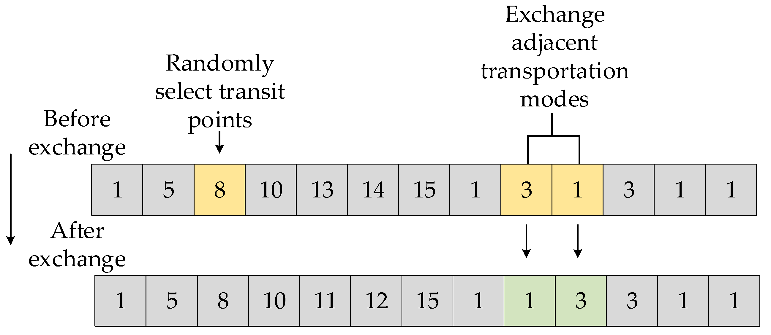
$Neighborhood$ operates by generating perturbed solutions through systematic application of predefined neighborhood operators to incumbent solutions, followed by rigorous validity verification procedures. Within this algorithmic architecture, four distinct neighborhood structures are implemented, with each whale agent stochastically selecting one operator per iteration under a uniform probability distribution across all available neighborhood transformation mechanisms.

The neighborhood search operators comprise four distinct mechanisms: Transport Mode Mutation stochastically selects a path segment and substitutes its current transport mode with an alternative viable option from available modes; Transshipment Node Insertion randomly identifies an insertion position, validates potential intermediate nodes maintaining bidirectional connectivity with adjacent nodes, inserts a qualified transshipment node, and assigns randomized transport modes to newly formed segments; Path Segment Reconfiguration selects a subpath for topological restructuring by exploring alternative nodal sequences and connectivity patterns to discover optimized routing configurations; Intermodal Transition Swap randomly selects a transshipment node and exchanges transport modes between its preceding and succeeding path segments, with operational schematics respectively illustrated in Figure 6, Figure 7, Figure 8 and Figure 9, demonstrating constrained stochastic perturbations that maintain network feasibility while enhancing solution diversity.

The variable neighborhood search (VNS) algorithm operates as a local search metaheuristic that systematically explores multiple predefined neighborhood structures around incumbent solutions to identify superior candidates, thereby refining selected individuals within the evolutionary population. Through cyclic activation of distinct neighborhood operators, it implements conditional transition logic: successful improvement triggers reversion to the primary neighborhood for intensified search, while exhaustive exploration without progress prompts sequential neighborhood switching. This hierarchical search protocol synergistically enhances solutions initially generated by the whale optimization algorithm’s tripartite position update strategies, enabling comprehensive solution space exploration that mitigates local optima entrapment risks. The mechanism probabilistically elevates global convergence likelihood while improving solution quality metrics through adaptive balance between intensification and diversification across dynamically reconfigured search landscapes.

In summary, the methodological workflow of the IWOA proposed in this study is systematically illustrated in Figure 10, delineating the synergistic integration of discrete encoding mechanisms, Sobol sequence initialization, hybrid crossover operators, and variable neighborhood search strategies within the algorithmic architecture.

5. Numerical Example

5.1. Data Preparation

In order to verify the effectiveness of the model and the accuracy of the algorithm, based on the existing research in relevant references [40], a case of a multimodal transport network with 14 nodes and 37 transport routes is constructed. The network is chosen to balance model complexity and computational feasibility, incorporating real-world multimodal features while aligning with benchmark scales in prior research for comparability. Assuming that the freight transportation demand is 20 TEU, it is transported from node 1 to node 14. The values of relevant parameters are shown in

Table 3. Transportation distance of different transportation modes between nodes in the network.

Number	Transportation Route	Road (km)	Railway (km)	Waterway (km)
1	1-2	332	735	—
2	1-3	306	786	—
3	1-4	281	540	638
4	2-3	814	606	—
5	2-5	569	427	346
6	2-6	687	745	496
7	2-7	402	390	—
8	2-8	429	386	—
9	3-4	1026	817	—
10	3-5	938	816	506
11	3-6	860	795	—
12	3-7	796	864	—
13	3-8	987	1035	1108
14	4-5	712	569	—
15	4-6	994	842	1084
16	4-7	613	775	—
17	4-8	805	613	—
18	5-9	413	574	825
19	5-10	543	413	—
20	6-9	634	695	474
21	6-10	625	752	304
22	7-9	327	432	—
23	7-10	455	516	866
24	8-9	435	508	—
25	8-10	396	487	—
26	9-10	341	346	—
27	9-11	478	584	542
28	9-12	535	617	—
29	9-13	677	585	—
30	10-11	1048	956	—
31	10-12	1178	1032	1245
32	10-13	988	1087	—
33	11-12	856	928	—
34	11-14	324	743	893
35	12-13	598	607	345
36	12-14	408	684	—
37	13-14	307	804	921

note—indicates that it does not exist.

,

Table 4. Transportation parameters of different transportation modes.

Mode of Transport	Speed (km/h)	Transportation Price (CNY/TEU·km)	Transport Carbon Emissions (kg/TEU·km)	Departure Interval (h)
Road	(40,90,100)	4.74	3.73	—
Railway	(45,50,75)	1.84	1.27	1
Waterway	(20,25,40)	0.89	0.42	1

note—indicates that it does not exist.

,

Table 5. Transit parameters of different transportation modes.

Mode of Transport	Transit Price (CNY/TEU)	Transfer Carbon Emission Coefficient (kg/TEU)
Road-Railway	150	2.17
Road-Waterway	100	1.98
Railway-Waterway	200	1.92

and

Table 6. Full load value and average daily depreciation rate of different categories of cargo.

Number	Type of Cargo	Name of Cargo	Price of Cargo (104 USD/TEU)	Average Daily Depreciation Rate (%)
n = 1	High value-added and timeliness-strong cargo	Mobile phones, tablets, etc.	40	0.043
n = 2	High value-added and timeliness-weak cargo	Precious metals, etc.	30	0.0012
n = 3	Low value-added and timeliness-strong cargo	Flowers, fruits, etc.	10	0.1
n = 4	Low value-added and timeliness-weak cargo	Ore raw materials, etc.	5	0.001

, and the structure of the multimodal transport network is shown in Figure 11. It is set that the transfer capacity of each node is the same, which is 50 TEU/h, the transfer and connection speed within the node is 40 km/h, the average connection distance is 10 km, and the goods need to complete the transportation task within 150 h. This study parameterizes the departure time for all transport modes at Node 1 as 8:00 AM, establishing a unified temporal reference point. Given that inter-nodal transit duration is mathematically determined by the quotient of transportation distance and velocity, we operationalize fuzzy transit duration calculation through modal-specific fuzzy velocity parameters under fixed geographical distances.

To systematically analyze transportation pricing dynamics, this study constructs 16 distinct freight rate scenario combinations to investigate the impact of cost volatility on route optimization outcomes, with detailed scenario parameterization presented in

Table 7. Transportation scenario settings.

Transportation Scenario	Parameter Value	Transportation Scenario	Parameter Value
1	0.6$c_{ij}^1$, 0.8$c_{ij}^2$	9	1.3$c_{ij}^1$, 0.8$c_{ij}^2$
2	0.6$c_{ij}^1$, 0.9$c_{ij}^2$	10	1.3$c_{ij}^1$, 0.9$c_{ij}^2$
3	0.6$c_{ij}^1$, 1.1$c_{ij}^2$	11	1.3$c_{ij}^1$, 1.1$c_{ij}^2$
4	0.6$c_{ij}^1$, 1.2$c_{ij}^2$	12	1.3$c_{ij}^1$, 1.2$c_{ij}^2$
5	0.7$c_{ij}^1$, 0.8$c_{ij}^2$	13	1.4$c_{ij}^1$, 0.8$c_{ij}^2$
6	0.7$c_{ij}^1$, 0.9$c_{ij}^2$	14	1.4$c_{ij}^1$, 0.9$c_{ij}^2$
7	0.7$c_{ij}^1$, 1.1$c_{ij}^2$	15	1.4$c_{ij}^1$, 1.1$c_{ij}^2$
8	0.7$c_{ij}^1$, 1.2$c_{ij}^2$	16	1.4$c_{ij}^1$, 1.2$c_{ij}^2$

.

5.2. Result Analysis

The IWOA was implemented in MATLAB R2021a, with core parameters configured as follows: initial population size = 100, maximum iteration threshold = 100, VNS adoption rate = 0.05, and elitism preservation rate = 0.05.

5.2.1. Algorithm Validity Test

Utilizing the aforementioned case study framework, a comprehensive comparative analysis was conducted between the whale optimization algorithm (WOA) and the improved whale optimization algorithm (IWOA) to evaluate algorithmic performance metrics. Both algorithms were systematically configured with identical population sizes (N = 100) and maximum iteration thresholds (T = 100) to ensure experimental parity. Through systematic validation involving 100 experimental trials, critical performance indicators, including convergence behavior and computational efficiency, were rigorously assessed. Experimental results (Figure 12) demonstrate that IWOA achieves solution convergence with an average of 8 iterations (standard error = 0.95), significantly outperforming WOA’s average convergence at 16 iterations (standard error = 1.77). Figure 13 illustrates a representative iteration process, revealing that IWOA’s initial solutions exhibit superior proximity to optimal values while demonstrating enhanced convergence velocity compared to WOA’s gradual convergence pattern. Notably, both algorithms successfully terminate within 50 iterations, with IWOA displaying accelerated convergence dynamics and improved solution stability. These empirical findings substantiate the efficacy of the proposed algorithmic enhancements in optimizing global search capabilities while significantly improving convergence efficiency and robustness in multimodal transportation optimization scenarios.

5.2.2. Model Solution Results

Experimental results demonstrate that under carbon emission-excluded scenarios, optimal transportation strategies for different cargo types exhibit distinct characteristics, as detailed in

Table 8. Optimal transportation scheme for different types of cargo.

Type of Cargo	Transportation Route	Mode of Transport	Total Cost (CNY)	Total Time (h)	Carbon Emissions (kg)
n = 1	1-2-7-9-13-14	H-R-R-R-H	160,857.12	38.41	83,494
n = 2	1-2-6-9-11-14	R-W-W-W-W	87,732.70	114.72	38,909
n = 3	1-2-7-9-12-14	R-R-R-R-R	132,215.62	58.68	72,593
n = 4	1-2-6-9-11-14	R-W-W-W-W	70,844.38	114.72	38,909

. Time-sensitive cargo demonstrates a “time-priority” pattern characterized by shorter transportation cycles accompanied by elevated carbon emissions and economic costs, whereas low time-sensitivity cargo adopts a “cost-priority” approach, predominantly utilizing waterway transportation to minimize transportation expenses.

This study conducts a comparative differential analysis of high-value, timeliness-strong cargo transportation strategies under distinct carbon emission policies. Under carbon taxation regimes, the optimal transportation strategy exhibits phased evolution with progressive tax increments. The solution results are shown in

Table 9. Changes of optimal transportation scheme under different carbon tax values.

Carbon Tax Rate (CNY/kg)	Transportation Scheme	Total Cost (CNY)	Carbon Emissions (kg)	Proportion of Carbon Emission Cost
0.1	1-H-2-R-7-R-9-R-13-H-14	169,206.5	83,494	4.93%
0.5	1-R-2-R-7-R-9-R-13-H-14	201,693.5	77,352	19.17%
1	1-R-2-R-7-R-9-W-11-H-14	239,666.3	68,349	28.52%
2	1-R-2-W-6-W-9-W-11-W-14	289,033.9	38,909	26.92%
3	1-R-2-W-6-W-9-W-11-W-14	327,943.3	38,909	35.59%
4	1-W-4-W-6-W-9-W-11-W-14	377,825.9	30,500	32.29%
5	1-W-4-W-6-W-9-W-11-W-14	398,246.3	30,500	38.29%

and as illustrated in Figure 14. When the tax rate reaches 0.1 CNY/kg, the optimal solution remains identical to the baseline scenario; at 1 CNY/kg, the optimal strategy shifts from road–rail intermodal to road–rail–water intermodal transportation, reducing carbon emissions by 11.63%; at 2 CNY/kg, emissions decrease by 43% with a 1.6 percentage point reduction in emission cost proportion within total expenditures. Strategic stability emerges between 2 and 3 CNY/kg, where tax adjustments fail to alter routing decisions. However, when the tax rate escalates to 4 CNY/kg, the optimal strategy transitions to exclusive waterway transportation, achieving minimal emissions of 30,500 kg (63.47% reduction versus baseline) while incurring 134% cost inflation. The findings demonstrate that moderate carbon tax escalation effectively promotes modal shift toward sustainable transportation structures, whereas excessive taxation achieves significant emission reductions at prohibitive economic costs, necessitating scientifically calibrated carbon taxation standards and implementation frameworks to guide multimodal transportation systems toward low-carbon development.

Under carbon trading and mandatory emission policies, analytical results demonstrate that total operational costs exhibit an upward trajectory with decreasing emission allowances and increasing carbon prices. When carbon prices reach zero, optimal costs under both policies align with baseline scenario outcomes. As emission caps descend below the minimum emissions threshold of feasible solutions, total costs surge exponentially with carbon price escalation, converging with carbon taxation model results at zero emission allowance. Three distinct operational regimes emerge: (1) Below 30,000 kg emission caps, costs escalate rapidly with carbon price increases; (2) between 30,000 and 40,000 kg caps, cost growth moderates as multimodal combinations partially offset carbon pricing impacts despite suboptimal time–value costs; and (3) above 40,000 kg caps, transportation cost stability enables progressive total cost reduction with carbon price rises. The results are shown in Figure 15.

Under carbon offset mechanisms, transportation schemes remain carbon price-insensitive when caps exceed baseline emissions due to non-tradable surplus allowances. For caps between baseline and minimum emission levels, adaptive multimodal strategies emerge through dynamic allowance–price optimization, demonstrating cost reduction and stabilization with expanding allowances. These findings necessitate comprehensive consideration of allowance–price dynamics, multimodal configuration interactions, and cargo-specific attributes when formulating transportation strategies under emission-constrained operational frameworks.

Under the mandatory carbon emission policy with allowance caps parameterized between 30,000 and 90,000 kg (increment: 10,000 kg), the evolution of optimal transportation strategies is systematically documented in

Table 10. Changes of optimal transportation scheme under mandatory carbon emission policy.

Carbon Quota (kg)	Transportation Scheme	Total Cost (CNY)	Total Time (h)
30,000	—	—	—
40,000	1-W-4-R-5-W-9-W-11-W-14	240,374.51	132.72
50,000	1-H-2-W-6-W-9-W-11-W-14	201,564.58	102.72
60,000	1-H-2-R-7-R-9-W-11-W-14	190,081.62	80.72
70,000	1-R-2-R-7-R-9-R-11-R-14	171,317.29	59.58
80,000	1-R-2-R-7-R-9-R-13-R-14	163,017.26	48.41
90,000	1-H-2-R-7-R-9-R-13-H-14	160,857.12	38.41

note—indicates that it does not exist.

. When the emission cap is set at 30,000 kg, no feasible solution exists, indicating all potential routes exceed this constraint. Progressive cap increases from 30,000 kg to 90,000 kg induce strategic shifts from the initial “1-W-4-R-5-W-9-W-11-W-14” configuration to the optimized “1-H-2-R-7-R-9-R-13-H-14” scheme, achieving 33% cost reduction and 71% transit time improvement while incurring significant carbon emission increases. Strategic stabilization occurs beyond 90,000 kg caps. This policy demonstrates dual regulatory effects as a rigid constraint mechanism: (1) loosened caps incentivize economically favorable but environmentally detrimental modal combinations with reduced transit durations; (2) cargo-type differential responses emerge—for time-insensitive shipments dominated by maritime transport in baseline scenarios, carbon cap adjustments exert limited impacts on modal selection and cost structures. Practical implementation requires comprehensive integration of transportation demand patterns and market dynamics with environmental constraints.

Under hybrid uncertainty conditions with temporal confidence level parameterized at 0.8 and regret coefficient set to 0.25, the robust optimization analysis yields critical findings as documented in

Table 11. Optimal transportation scheme and robust optimal solution under various transportation scenarios.

Scenario	Optimal Transportation Scheme	Scenario-Optimal Total Cost (CNY)	Robust-Optimal Total Cost (CNY)	Regret Value (%)
1	1-H-2-R-7-R-9-R-13-H-14	117,104	120,958	3.29
2	1-H-2-R-7-R-9-R-13-H-14	121,719	12,798	5.15
3	1-H-2-H-7-H-9-H-11-H-14	131,390	156,087	18.8
4	1-H-2-H-7-H-9-H-11-H-14	135,116	16,372	21.17
5	1-H-2-R-7-R-9-R-13-H-14	123,162	123,868	0.57
6	1-H-2-R-7-R-9-R-13-H-14	127,777	130,894	2.44
7	1-H-2-R-7-R-9-R-13-H-14	146,237	158,997	8.73
8	1-H-2-H-7-H-9-H-11-H-14	149,051	16,602	11.39
9	1-R-2-R-7-R-9-R-12-R-14	126,115	142,495	12.99
10	1-R-2-R-7-R-9-R-12-R-14	135,490	149,520	10.36
11	1-R-2-R-7-R-9-R-12-R-14	17,298	177,623	2.68
12	1-R-2-R-7-R-9-R-12-R-14	182,361	184,650	1.25
13	1-R-2-R-7-R-9-R-12-R-14	126,115	145,405	15.3
14	1-R-2-R-7-R-9-R-12-R-14	13,549	152,431	12.5
15	1-R-2-R-7-R-9-R-12-R-14	172,987	180,534	4.36
16	1-R-2-R-7-R-9-R-12-R-14	182,361	187,560	2.85

. The robust optimal transportation scheme “1-Rail-2-Rail-7-Rail-9-Rail-13-Road-14” demonstrates an expected total cost of CNY 154,297, accompanied by an average regret value of 0.06 and maximum regret value of 0.21 across all pricing scenarios. This solution maintains comprehensive transportation cost deviations within the predefined 0.25 regret coefficient threshold relative to robust objective function values across all operational scenarios, thereby satisfying robust feasibility criteria. Comparative analysis reveals strategic divergence between baseline and robust optimal solutions in both nodal sequences and modal combinations, highlighting the methodology’s capacity to systematically address multimodal uncertainties. The identified scheme achieves cost-efficient robustness through balanced integration of railway dominance and strategic road transportation terminal legs, effectively mitigating pricing volatility impacts while maintaining temporal reliability under constrained confidence parameters.

Based on the analytical results, critical parameters for the four low-carbon policy models were systematically configured: carbon tax rate at CNY 0.4/kg, mandatory emission cap at 70,000 kg, carbon trading/offset caps at 75,000 kg, and carbon price at CNY 0.3/kg. The comparative results (Figure 16) reveal differentiated policy impacts on environmental performance, economic costs, and decision stability under uncertainty. Regarding emission reductions, the baseline model exhibits the highest carbon output due to absent policy constraints. All low-carbon policies demonstrate emission mitigation efficacy with varying intensities: the mandatory policy achieves 11.63% reduction through rigid constraints, while tax, trading, and offset policies yield equivalent 6.15% reductions via market mechanisms.

Economic analysis demonstrates tradeoff patterns: carbon taxation incurs 23.7% cost inflation alongside emission reductions; trading/offset policies maintain balanced cost-emission ratios; and the mandatory policy shows intermediate cost escalation, reflecting cost-environment equilibrium under regulatory constraints. Decision stability metrics reveal maximum regret values of 18.2% for baseline and 21.5% for tax policy, contrasted with elevated values under trading and offset mechanisms due to market complexity. The mandatory policy enhances stability through deterministic constraints. The comparative conditions of total costs, carbon emissions, and stability under different policies are shown in

Table 12. Comparison of the results of the regret coefficient change.

Policy Type	Cost	Emissions	Stability
Carbon Tax Policy	High	Medium	Medium
Carbon Trading Policy	Low	Medium	High
Mandatory Carbon Emission Policy	Medium	Low	Low
Carbon Offset Policy	Medium	Medium	High

. These findings highlight policy-specific optimization frontiers: mandatory constraints prioritize environmental rigor with moderate economic impacts; market-based mechanisms balance flexibility and sustainability; and taxation emphasizes emission control at higher costs. Strategic selection should integrate emission reduction targets, budgetary constraints, and operational risk tolerance to formulate context-specific decarbonization roadmaps for multimodal transportation systems.

5.2.3. Sensitivity Analysis

The regret coefficient, functioning as a pivotal risk metric, effectively balances economic efficiency and operational reliability in transportation planning. Comparative analysis of regret coefficient variations (

Table 13. Comparison of the results of the regret coefficient change.

Regret Coefficient	Robust Optimal Transportation Scheme	Expected Total Cost	Maximum Regret Value
0.2	—	—
0.3	1-R-2-R-7-R-9-R-13-H-14	154,297	0.21
0.4	1-R-2-R-7-R-9-R-13-R-14	154,138	0.34
0.5	1-H-2-R-7-R-9-R-13-H-14	154,025	0.46
0.6	1-H-2-R-7-R-9-R-13-H-14	154,025	0.46

) reveals three operational regimes: (1) No feasible solutions emerge below 0.2, indicating excessively stringent constraints; (2) between 0.3 and 0.5, robust optimal strategies evolve with decreasing total costs (12.7% reduction from 0.3 to 0.5), demonstrating that lower coefficients correspond to conservative strategies with cost premiums (18.3% higher than baseline), while higher coefficients enable risk-tolerant decision-making with cost optimization; and (3) beyond 0.5, strategic configurations stabilize despite coefficient increases. This parametric sensitivity analysis establishes a flexible decision-making mechanism allowing systematic navigation from complete risk aversion to managed risk acceptance through coefficient calibration. Such adaptive optimization proves particularly advantageous for container multimodal transportation systems exposed to stochastic disruptions like port congestion and scheduled service delays, enabling balanced tradeoffs between cost containment and service reliability under uncertainty.

The time confidence level $\alpha$ represents the decision-maker’s preference attitude towards the transportation time risk, and is used to measure the degree of trust in the “reliable part” of the triangular fuzzy number. In the above-mentioned example, with other conditions remaining unchanged, the robust total cost and the maximum regret value obtained by changing $\alpha$ are shown in Figure 17. When $\alpha$ increases, the total cost rises, indicating that the decision-maker tends to be conservative. In this case, it corresponds to a longer transportation time and lower risk, which is suitable for scenarios with high requirements for transportation stability. When $\alpha$ decreases, the total cost drops, and the decision-maker tends to take risks. At this time, it corresponds to a shorter transportation time, which is suitable for scenarios with high requirements for timeliness. When $\alpha =0.5$, the decision-maker has a relatively balanced consideration of the transportation time risk and the transportation cost economy. At this time, the maximum regret value in all scenarios is the smallest. As $\alpha$ increases or decreases, the maximum regret value keeps increasing, indicating that the volatility of the transportation plan is greater. Decision-makers need to flexibly set $\alpha$ according to the specific needs of multimodal transportation to balance the risk of time fluctuations and the cost.

6. Conclusions

This study proposes a containerized low-carbon multimodal transportation path optimization model under dual-factor hybrid uncertainties, incorporating railway schedule constraints, maritime departure regularity, and cargo-specific time–value costs. The IWOA demonstrates enhanced global and local search capabilities compared to conventional WOA, with experimental validation confirming its applicability to complex transportation optimization problems.

This study provides actionable insights for governmental bodies formulating transportation policies and multimodal transport operators designing logistics solutions. Crucially, our findings emphasize the necessity of concurrently addressing dual uncertainties—freight rate volatility and temporal efficiency—during route and mode selection. To this end, we propose a novel low-carbon routing framework under hybrid uncertainty, featuring robust policy-adaptive capabilities. By flexibly calibrating key parameters (e.g., unit carbon price, emission allowances), the framework dynamically responds to regional decarbonization mandates, enabling context-specific decision support. Furthermore, our methodology extends to designing carbon-conscious transport schemes for diverse cargo value profiles, establishing theoretical foundations for differentiated logistics strategies.

Notwithstanding these contributions, certain limitations warrant acknowledgment. While addressing cost and time uncertainties, the model assumes mutual independence between these stochastic factors and simplifies secondary parameter interactions. These necessary abstractions may constrain predictive accuracy in extreme or highly complex scenarios. Additionally, parameter calibration relies on historical datasets, partial assumptions, and the existing literature, potentially introducing deviations when applied across heterogeneous regulatory environments and industry standards. Although our case study aligns with prior computational tractability conventions, model scalability across large-scale networks requires further validation.

Building upon this foundation, we recommend that future work investigate the impacts of carbon price volatility by quantifying the currently unmodeled effects of dynamic carbon pricing on routing decisions, as well as develop enhanced optimization schemes by constructing more realistic models that capture complex multi-factor interdependencies to significantly increase practical utility. These priorities will guide our subsequent research endeavors.

References

1. Ahmady, M.; Yeghaneh, Y.E. Optimizing the Cargo Flows in Multi-modal Freight Transportation Network Under Disruptions. Iran. J. Sci. Technol.-Trans. Civ. Eng. 2022, 46, 453–472. [Google Scholar] [CrossRef]
2. Dini, N.; Yaghoubi, S.; Bahrami, H. Logistics Performance Index-driven in operational planning for logistics companies: A smart transportation approach. Transp. Policy 2025, 160, 42–62. [Google Scholar] [CrossRef]
3. Shramenko, N.; Muzylyov, D.; Shramenko, V. Methodology of costs assessment for customer transportation service of small perishable cargoes. Int. J. Bus. Perform. Manag. 2020, 21, 132–148. [Google Scholar] [CrossRef]
4. Solano-Charris, E.L.; Prins, C.; Santos, A.C. Solving the bi-objective robust vehicle routing problem with uncertain costs and demands. RAIRO-Oper. Res. 2016, 50, 689–714. [Google Scholar] [CrossRef]
5. Amine Masmoudi, M.; Baldacci, R.; Mancini, S.; Kuo, Y.-H. Multi-compartment waste collection vehicle routing problem with bin washer. Transp. Res. Part E Logist. Transp. Rev. 2024, 189, 103681. [Google Scholar] [CrossRef]
6. Chang, T.S. Best routes selection in international intermodal networks. Comput. Oper. Res. 2008, 35, 2877–2891. [Google Scholar] [CrossRef]
7. Raicu, S.; Popa, M.; Costescu, D. Uncertainties Influencing Transportation System Performances. Sustainability 2022, 14, 7660. [Google Scholar] [CrossRef]
8. Christ, N.; Ferrantino, M.J. Land Transport for Export: The Effects of Cost, Time, and Uncertainty in Sub-Saharan Africa. World Dev. 2011, 39, 1749–1759. [Google Scholar] [CrossRef]
9. Fattahi, Z.; Behnamian, J. Location and transportation of intermodal hazmat considering equipment capacity and congestion impact: Elastic method and sub-population genetic algorithm. Ann. Oper. Res. 2022, 316, 303–341. [Google Scholar] [CrossRef]
10. Ba, Y.L.; Feng, C.X.; Jia, W.P.; Liu, X.; Ren, J.W. A Multi-Scenario Optimization Model for Emergency Cold Chain Logistics Distribution. Math. Probl. Eng. 2021, 2021, 9. [Google Scholar] [CrossRef]
11. Luo, Y.; Zhang, Y.G.; Huang, J.X.; Yang, H.Y. Multi-route planning of multimodal transportation for oversize and heavyweight cargo based on reconstruction. Comput. Oper. Res. 2021, 128, 13. [Google Scholar] [CrossRef]
12. Lasota, M.; Jacyna, M.; Szacillo, L. Fault tree method as a decision-making tool for assessing the risks of transportation of dangerous loads. Sci. J. Sil. Univ. Technol.-Ser. Transp. 2024, 123, 133–154. [Google Scholar] [CrossRef]
13. Ozbiltekin-Pala, M.; Kazancoglu, Y.; Karamperidis, S.; Ram, M. Managing the risks against carbon neutralization for green maritime transport. J. Clean. Prod. 2024, 457, 11. [Google Scholar] [CrossRef]
14. Basso, L.J.; Jara-Díaz, S.R. Integrating congestion pricing, transit subsidies and mode choice. Transp. Res. Part A Policy Pract. 2012, 46, 890–900. [Google Scholar] [CrossRef]
15. Chen, X.H.; Hu, X.H.; Liu, H.B. Low-carbon route optimization model for multimodal freight transport considering value and time attributes. Socio-Econ. Plan. Sci. 2024, 96, 16. [Google Scholar] [CrossRef]
16. Kaewfak, K.; Ammarapala, V.; Huynh, V.N. Multi-objective Optimization of Freight Route Choices in Multimodal Transportation. Int. J. Comput. Intell. Syst. 2021, 14, 794–807. [Google Scholar] [CrossRef]
17. Pustiulha, S.; Samchuk, V.; Holovachuk, I.; Prydiuk, V.; Klak, Y. Methodology for Selecting Optimal Routes for the Transportation of Dangerous Goods in Conditions of Risk Uncertainty. Transp. Telecommun. J. 2024, 25, 150–160. [Google Scholar] [CrossRef]
18. Li, L.; Zhang, Q.; Zhang, T.; Zou, Y.; Zhao, X. Optimum Route and Transport Mode Selection of Multimodal Transport with Time Window under Uncertain Conditions. Mathematics 2023, 11, 3244. [Google Scholar] [CrossRef]
19. Koohathongsumrit, N.; Chankham, W. A hybrid approach of fuzzy risk assessment-based incenter of centroid and MCDM methods for multimodal transportation route selection. Cogent Eng. 2022, 9, 31. [Google Scholar] [CrossRef]
20. Sun, L.S.; Karwan, M.H.; Kwon, C. Robust Hazmat Network Design Problems Considering Risk Uncertainty. Transp. Sci. 2016, 50, 1188–1203. [Google Scholar] [CrossRef]
21. Zhang, W.; Jenelius, E.; Ma, X.L. Freight transport platoon coordination and departure time scheduling under travel time uncertainty. Transp. Res. Part E Logist. Transp. Rev. 2017, 98, 1–23. [Google Scholar] [CrossRef]
22. Avila-Torres, P.; Caballero, R.; Litvinchev, I.; Lopez-Irarragorri, F.; Vasant, P. The urban transport planning with uncertainty in demand and travel time: A comparison of two defuzzification methods. J. Ambient Intell. Humaniz. Comput. 2018, 9, 843–856. [Google Scholar] [CrossRef]
23. Dhanasekar, S.; Rani, J.J.; Annamalai, M. Transportation Problem for Interval-Valued Trapezoidal Intuitionistic Fuzzy Numbers. Int. J. Fuzzy Log. Intell. Syst. 2022, 22, 155–168. [Google Scholar] [CrossRef]
24. Xu, Q.; Yan, Y.; Huang, J.; Chen, X.Y.; Cheng, R.; Yin, X.Y.; Yang, Z.Z. Optimization on Container Drayage Scheduling in Stochastic Time-dependent Network. J. Mar. Sci. Technol. 2024, 32, 20. [Google Scholar] [CrossRef]
25. Rahiminia, S.; Mehrabi, A.; Jabbarzadeh, A.; Aghaee, M.P. A hybrid optimization approach for designing sustainable intermodal freight transport under mixed uncertainty. Socio-Econ. Plan. Sci. 2025, 98, 18. [Google Scholar] [CrossRef]
26. Zhang, X.; Jin, F.Y.; Yuan, X.M.; Zhang, H.Y. Low-Carbon Multimodal Transportation Path Optimization under Dual Uncertainty of Demand and Time. Sustainability 2021, 13, 8180. [Google Scholar] [CrossRef]
27. Yang, L.; Zhang, C.; Wu, X. Multi-Objective Path Optimization of Highway-Railway Multimodal Transport Considering Carbon Emissions. Appl. Sci. 2023, 13, 4731. [Google Scholar] [CrossRef]
28. Wu, C.Y.; Zhang, Y.G.; Xiao, Y.; Mo, W.W.; Xiao, Y.X.; Wang, J. Optimization of Multimodal Paths for Oversize and Heavyweight Cargo under Different Carbon Pricing Policies. Sustainability 2024, 16, 6588. [Google Scholar] [CrossRef]
29. Cheng, M.Y.; Dong, L.M. An Evolutionary Multitasking Ant Colony Optimization Method Based on Population Diversity Control for Multimodal Transport Problems. Int. J. Comput. Intell. Syst. 2024, 17, 15. [Google Scholar] [CrossRef]
30. Haris, M.; Nam, H. Path Planning Optimization of Smart Vehicle with Fast Converging Distance-Dependent PSO Algorithm. IEEE Open J. Intell. Transp. Syst. 2024, 5, 726–739. [Google Scholar] [CrossRef]
31. Li, M.; Sun, X. Path Optimization of Low-Carbon Container Multimodal Transport under Uncertain Conditions. Sustainability 2022, 14, 14098. [Google Scholar] [CrossRef]
32. Liu, Z.W.; Zhou, S.H.; Liu, S. Optimization of Multimodal Transport Paths Considering a Low-Carbon Economy Under Uncertain Demand. Algorithms 2025, 18, 92. [Google Scholar] [CrossRef]
33. Wang, X.Y.; Zhang, P.; Du, Z.G.; Tian, A.Q.; Lv, H.X. Research on Optimization of International Multimodal Transportation Routes Based on Uncertainty Theory. Transp. Res. Record 2024, 2678, 798–821. [Google Scholar] [CrossRef]
34. Niksirat, M.; Ghatee, M.; Hashemi, S.M. Multimodal K-shortest viable path problem in Tehran public transportation network and its solution applying ant colony and simulated annealing algorithms. Appl. Math. Model. 2012, 36, 5709–5726. [Google Scholar] [CrossRef]
35. Zhu, P.; Lv, X.; Shao, Q.; Kuang, C.; Chen, W. Optimization of Green Multimodal Transport Schemes Considering Order Consolidation under Uncertainty Conditions. Sustainability 2024, 16, 6704. [Google Scholar] [CrossRef]
36. Mohammadi, M.; Jula, P.; Tavakkoli-Moghaddam, R. Design of a reliable multi-modal multi-commodity model for hazardous materials transportation under uncertainty. Eur. J. Oper. Res. 2017, 257, 792–809. [Google Scholar] [CrossRef]
37. Shojaie, A.A.; Raoofpanah, H. Solving a two-objective green transportation problem by using meta-heuristic methods under uncertain fuzzy approach. J. Intell. Fuzzy Syst. 2018, 34, 1–10. [Google Scholar] [CrossRef]
38. Koohathongsumrit, N.; Meethom, W. A Fuzzy Decision-Making Framework for Route Selection in Multimodal Transportation Networks. EMJ-Eng. Manag. J. 2022, 34, 689–704. [Google Scholar] [CrossRef]
39. Mirjalili, S.; Lewis, A. The Whale Optimization Algorithm. Adv. Eng. Softw. 2016, 95, 51–67. [Google Scholar] [CrossRef]
40. Deng, M.J.; Dai, Y.Z.; Li, X. Robust Optimization of Multi-modal Transportation Routing with Low-carbonunder Demand Uncertainty. Ind. Eng. J. 2023, 26, 104–113. [Google Scholar]
Figure 1. Three sequential phases in the development of the model architecture.
Applsci 15 06894 g001
Figure 2. Membership function of triangular fuzzy numbers.
Applsci 15 06894 g002
Figure 3. Schematic diagram of coding structure.
Applsci 15 06894 g003
Figure 4. Single point crossing.
Applsci 15 06894 g004
Figure 5. Double point crossing.
Applsci 15 06894 g005
Figure 6. Variation of the transportation mode.
Applsci 15 06894 g006
Figure 7. Transit node insertion.
Applsci 15 06894 g007
Figure 8. Path segment reorganization.
Applsci 15 06894 g008
Figure 9. Exchange the adjacent transportation modes of the transit node. Variable Neighborhood Search Strategy (VNS).
Applsci 15 06894 g009
Figure 10. The process of IWOA.
Applsci 15 06894 g010
Figure 11. Multimodal transport network structure.
Applsci 15 06894 g011
Figure 12. Comparison of the algorithm-solving efficiency.
Applsci 15 06894 g012
Figure 13. Single iteration comparison.
Applsci 15 06894 g013
Figure 14. Total cost, carbon emissions, and carbon emission cost under different carbon tax values.
Applsci 15 06894 g014
Figure 15. Comparative analysis of cost responsiveness to carbon trading and carbon offset policy scenarios. (a) Variation of total cost as a function of carbon price and allowance allocation under carbon trading policy. (b) Variation of total cost as a function of carbon price and allowance allocation under carbon offset policy.
Applsci 15 06894 g015
Figure 16. Comparison of the results under different types of carbon policies.
Applsci 15 06894 g016
Figure 17. Effect of the period time confidence on total cost and maximum regret value.
Applsci 15 06894 g017