Accuracy of Vegetation Height and Terrain Elevation Derived from Terrestrial Ecosystem Carbon Inventory Satellite in Forested Areas

Abstract

Forest ecosystems serve as pivotal components of the global carbon cycle, with canopy height representing a critical biophysical parameter for quantifying ecosystem functionality, thereby holding substantial implications for forest resource management and carbon sequestration assessments. The precise extraction of ground elevation and vegetation canopy height is essential for advancing topographic and ecological research. The Terrestrial Ecosystem Carbon Inventory Satellite (referred to as TECIS hereafter) offers unprecedented capabilities for the large-scale, high-precision extraction of ground elevation and vegetation canopy height. Using the Northeast China Tiger and Leopard National Park as our study area, we first processed TECIS data to derive topographic and canopy height profiles. Subsequently, the accuracy of TECIS-derived ground and canopy height estimates was validated using onboard light detection and ranging (LiDAR) measurements. Finally, we systematically evaluated the influence of multiple factors on estimation accuracy. Our analysis revealed that TECIS-derived ground and canopy height estimates exhibited mean errors of 0.7 m and −0.35 m, respectively, with corresponding root mean square error (RMSE) values of 3.83 m and 2.70 m. Furthermore, slope gradient, vegetation coverage, and forest composition emerged as the dominant factors influencing canopy height estimation accuracy. These findings provide a scientific basis for optimizing the screening and application of TECIS data in global forest carbon monitoring.

1. Introduction

Forest ecosystems constitute a crucial component of global natural resources. As the largest terrestrial carbon pool, they contribute over 60% of terrestrial carbon sinks and play an irreplaceable role in regulating the climate and stabilizing the biosphere [1]. Tree height serves as a key factor that characterizes the vertical structure of forests. It is also an important indicator for assessing carbon stock, productivity, and ecosystem service functions [2,3,4], as well as for estimating biomass and evaluating forest health [5,6]. Therefore, it holds significant importance to acquire tree height information within forest systems in a rapid, real-time, and high-precision manner.

Tree height information is predominantly obtained via two approaches, namely manual ground-based surveys and remote sensing inversion [7]. Manual survey methods are capable of providing more precise forest data in low-density and sparse forests [8,9]. However, it proves challenging to acquire accurate information in forests featuring complex topography, intricate stand structures, and high vegetation coverage. In this study, topography refers to the physical characteristics of the land surface, including elevation, slope, and terrain features, which can significantly influence the accuracy of tree height measurements. Moreover, such surveys typically demand a substantial amount of time and labor [10]. To address the limitations of manual surveys, remote sensing technology, which boasts the advantages of extensive coverage and high precision, has been extensively utilized in recent years for the collection and monitoring of forest- related data, including that of various tree species [11,12]. Light detection and ranging (LiDAR) can be classified into ground-based LiDAR (TLS), airborne laser scanning (ALS), and satellite-borne LiDAR based on different platforms. ALS is capable of acquiring high-precision three-dimensional forest structural information and extracting forest features such as tree heights. Nevertheless, it is constrained by the flight altitude of the aircraft, route planning, and the high cost [13,14,15,16,17]. Satellite-borne LiDAR, on the contrary, is characterized by large-scale coverage and all-weather operability. This feature can guarantee the continuity and stability of the data. It also has robust anti-interference capabilities and can penetrate forest vegetation to provide information on the canopy stratification structure, understory vegetation, and the ground surface [15,18,19].

The Ice, Cloud, and Land Elevation Satellite (ICESat-1; 2003–2009) pioneered spaceborne full-waveform altimetry through its Geoscience Laser Altimeter System (GLAS), enabling unprecedented monitoring of polar elevation dynamics across glaciers, ice sheets, and sea ice [20]. As ICESat-1’s successor, ICESat-2 (launched September 2018) [21] features the Advanced Terrain Laser Altimeter System (ATLAS), employing photon-counting LiDAR technology with multi-beam micropulses at high repetition rates for three-dimensional along-track feature characterization [22,23]. Neuenschwander et al. [24] conducted accuracy assessments of extracted ground and canopy heights in Finnish forests, while Yu et al. [25] systematically analyzed influencing factors on ICESat-2’s height estimation accuracy. Their respective studies reported Bias of 0.28$\mathrm{m}$ (ground) and −0.21$\mathrm{m}$ (canopy), with corresponding RMSE values of 0.96$\mathrm{m}$ and 2.50$\mathrm{m}$. Launched in December 2018, the Global Ecosystem Dynamics Investigation (GEDI) [26] represents the first dedicated satellite LiDAR system for vegetation vertical structure monitoring, featuring superior technical specifications including reduced footprint diameter, enhanced sampling density, and improved resolution/sensitivity compared to conventional spaceborne LiDAR systems. However, its performance remains susceptible to slope, vegetation height, and beam sensitivity factors.

Launched from China’s Taiyuan Satellite Launch Center in August 2022, the Terrestrial Ecosystem Carbon Inventory Satellite (TECIS) represents China’s inaugural quantitative remote sensing satellite dedicated to terrestrial ecosystem monitoring. Equipped with the next-generation Carbon Sinks and Aerosol LiDAR (CASAL) as its primary payload—the nation’s first multi-beam full-waveform LiDAR system—TECIS specializes in the high-precision measurement of carbon stocks, forest resources, and productivity [27,28,29,30]. The satellite features an advanced payload configuration, including (1) the CASAL with dual-mode vegetation measurement and aerosol detection capabilities (see Figure 1 for operational schematic); (2) a directional multi-spectral camera (DMC) for spectral characterization; (3) a fluorescence spectral imager (FSI) for assessing vegetation physiological status; and (4) a directional polarization camera (DPC) for atmospheric correction. These payloads work synergistically to form a comprehensive Earth observation system. Pang et al. [31] validated TECIS’s forest monitoring capability through waveform analysis, demonstrating strong consistency between the satellite’s canopy parameters and the 75th percentile heights from airborne laser scanning (ALS) (random forest model: $R^2=0.85$, $RMSE=$1.38$\mathrm{m}$).

Table 1. Comparison of operational parameters for ICESat-1/GLAS, ICESat-2/ATLAS, GEDI, and TECIS LiDAR systems.

Parameters	ICESat-1/GLAS	ICESat-2/ATLAS	GEDI	TECIS/CASAL
Launch date	2003	2018.09	2018.12	2022.08
Platform	ICESat	ICESat-2	ISS	TECIS
Nominal altitude	600	500	405	506
Wavelength	1064/532	532	1064	1064
Pulse repetition	40	10	343	40
Ground tracks	1	6	8	5
Measurement concept	Full waveform	Photon counting	Full waveform	Full waveform
Footprint size	∼70$\mathrm{m}$	17$\mathrm{m}$	∼25$\mathrm{m}$	25$\mathrm{m}$
Along-track distance	170$\mathrm{m}$	0.7$\mathrm{m}$	60$\mathrm{m}$	180$\mathrm{m}$
Across-track distance	2.5–15 km	3.3	0.6	4

systematically compares the mission-critical parameters of four generations of spaceborne LiDARs-ICESat, ICESat-2, GEDI, and TECIS.

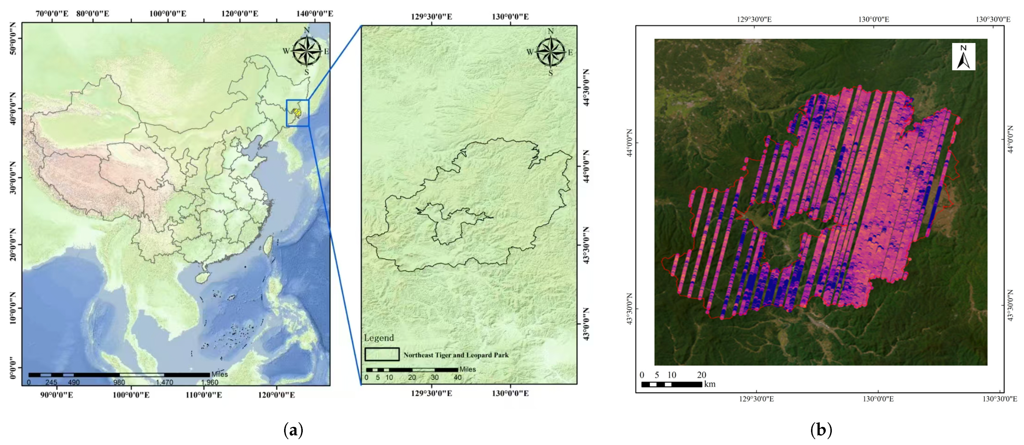
While forest canopy height inversion studies utilizing ICESat/GLAS and GEDI datasets have been extensively documented, research employing laser full-waveform data from domestic terrestrial carbon monitoring satellites remains comparatively limited. Given significant variations in payload hardware specifications, the performance of terrestrial carbon monitoring satellites for forest canopy height retrieval warrants comprehensive investigation. This study employs China’s Northeast Tiger and Leopard National Park as a test site to (1) evaluate the accuracy of CASAL-derived ground and canopy height estimates and (2) establish a methodological foundation for subsequent TECIS applications in forest canopy height and aboveground biomass quantification.

2. Materials and Methods

2.1. Study Area

The research was conducted in Northeast China Tiger and Leopard National Park (Figure 2), spanning geographical coordinates 129°5′ E–130°23′ E and 43°19′ N–44°10′ N, with a total area of approximately 5600 km². The region experiences a continental humid monsoon climate, characterized by windy and dry springs, short and hot summers, cool autumns with rapid temperature declines, and prolonged cold winters. The mean annual temperature is 5 °C, with annual precipitation ranging from 450 mm to 750 mm, predominantly concentrated between May and September. The terrain exhibits complex geomorphological diversity, primarily comprising low-to-medium mountains, valleys, and hills. The area harbors exceptionally rich temperate forest flora, with forest coverage reaching 93.32%. Dominant forest types include broadleaf forests, deciduous coniferous forests, and a limited proportion of evergreen coniferous forests. The extended winter season provides an extended temporal window for light detection and ranging (LiDAR) monitoring, while the structurally simplified and well-defined tree canopies during this period offer optimal data acquisition conditions.

2.2. Dataset

2.2.1. Carbon Sinks and Aerosol LiDAR Data

This study utilized 9 orbital passes of Terrestrial Ecosystem Carbon Inventory Satellite (TECIS) altimetry data acquired over the study area between October 2022 and April 2023 to assess laser altimetry elevation accuracy. Specific information is provided in

Table 2. List of CASAL datasets used in this study.

No.	Dataset ID
1	CM1_CASAL_A1_20221029_0000001309_L20000232387
2	CM1_CASAL_A1_20221103_0000001386_L20000231223
3	CM1_CASAL_A1_20221213_0000001993_L20000231221
4	CM1_CASAL_A1_20230102_0000002297_L20000337144
5	CM1_CASAL_A1_20230117_0000002525_L20000337174
6	CM1_CASAL_A1_20230206_0000002829_L20000337152
7	CM1_CASAL_A1_20230313_0000003361_L20000337159
8	CM1_CASAL_A1_20230318_0000003438_L20000337137
9	CM1_CASAL_A1_20230323_0000003513_L20000337167

. The L2 product provides comprehensive geospatial and waveform information, including longitude, latitude, elevation, full-waveform data, optical axis monitoring images, and ancillary data for each laser footprint. In-orbit calibration of TECIS demonstrates elevation measurement accuracy better than 0.7 m and horizontal positioning precision within 6 m [27]. To minimize non-forest area bias, we employed 30 m resolution GlobeLand30 land cover data to filter laser footprints, excluding non-forest areas from analysis. The final dataset comprised 21,784 validated laser footprints within the study area.

2.2.2. Airborne Laser Scanning Data

To validate Carbon Sinks and Aerosol LiDAR (CASAL) elevation estimation accuracy, we utilized airborne laser scanning (ALS) data acquired by a RIEGL VQ-1560i system (RIEGL Laser Measurement Systems, Horn, Austria) mounted on a Cessna 208B aircraft (Textron Aviation, Wichita, KS, USA) in August–September 2018. The data were referenced to the China Geodetic Coordinate System 2000 (CGCS2000) with elevation values based on the 1985 National Elevation Datum, projected using a 3° Gauss–Krüger coordinate system and acquired at a point density of 16 pulses/m2. Point cloud preprocessing, including noise removal and classification, was performed using LiDAR360 v2.2. Classified point clouds were interpolated via triangular irregular network (TIN) modeling to generate 1 m resolution digital surface models (DSMs) and a digital elevation model (DEM). To ensure elevation reference consistency, we performed datum conversion between the Universal Transverse Mercator (UTM) WGS84 coordinate system used for ALS products and the Geoid12A vertical datum, aligning them with the WGS84 ellipsoid reference of CASAL data prior to accuracy assessment.

2.3. Data Processing

In this paper, ALS forest canopy height and CASAL full-waveform forest canopy height were used for comparison, and the study was carried out in accordance with the following methodological steps: (1) accuracy analysis of all CASAL observation data; (2) accuracy analysis of different forest types; and (3) screening and analysis of effective factors affecting the performance of CASAL in forest areas. Data processing in this study can be divided into two parts, namely data preprocessing and statistical analysis. The data processing and statistical analysis were performed using Python v3.8, and the mapping visualization was achieved using ArcGIS v10.7. The data processing flow is illustrated in Figure 3.

2.3.1. Carbon Sinks and Aerosol LiDAR Data Processing

Footprint Screening

The accurate estimation of tree height using satellite-borne large-footprint LiDAR data requires rigorous quality control, as atmospheric interference (e.g., clouds, haze) and non-forested laser returns can significantly compromise measurement fidelity. To ensure data integrity, low-quality waveforms were filtered using quality assessment fields embedded in the CASAL L2 product, retaining only observations with a signal-to-noise ratio ($SNR$) > 5. The CASAL system operates in two gain modes (Fgain and Vgain); we exclusively analyzed Fgain-mode footprints due to their superior SNR characteristics. Footprints were geolocated using IndexNum and BLH fields, with non-forest returns excluded through spatial filtering. Only footprints meeting all quality criteria (flag > 0, rec_peaks > 1, and SNR > 5) were retained, ensuring valid echoes with detectable waveform peaks and sufficient signal quality. SNR was computed using Equation (1) [32] as follows:

$$SNR=10{log}_{10}{\displaystyle \frac{D{N}_{max}-N_{ave}}{\sigma }}$$

(1)

where $D{N}_{max}$ denotes the maximum waveform amplitude, $N_{ave}$ represents the mean background noise value, and $\sigma$ indicates the standard deviation of background noise. The fields involved in the screening criteria are detailed in

Table 3. Description of main parameters in CASAL LiDAR products.

Parameter	Directory	Description
IndexNum	Lasern/IndexNum	Laser waveform sequence number
BLH	Lasern/Location_Fgain/BLH	Geodetic coordinates: B: Latitude L: Longitude H: Elevation
Flag	Location_Fgain/Flag	Data quality flag
rec_peaks	Rec_waveform/Wf_Fgain/Characters/rec_peaks	Number of Gaussian components in fitted waveform
rec_Thr	Rec_waveform/Wf_Fgain/Characters/rec_Thr	Effective signal threshold calculated from raw echoes
rec_noise	Rec_waveform/Wf_Fgain/Characters/rec_noise	Mean background noise value of raw received echoes

. After applying these filters, a total of 18,321 valid laser footprints were retained for analysis.

Waveform Feature Parameter Extraction

Forest canopy height is typically derived by subtracting the ground elevation (corresponding to the last waveform peak) from the maximum elevation detected in the full waveform, with the resulting difference representing the maximum canopy height [33,34,35,36]. Using the extracted threshold value (rec_Thr) from the dataset, we identified the waveform signal boundaries by (1) defining SigBeg as the first position where backward signal strength from the initial data frame exceeds rec_Thr and (2) defining SigEnd as the first position where the forward signal strength from the terminal data frame surpasses rec_Thr.

The relative height (RH) metric represents the vertical distance from the cumulative energy percentage (0% to 100%) of the full waveform to the ground echo position [26,37]. It is commonly used to characterize the vertical structure of forest canopies and serves as a critical parameter in CASAL LiDAR data processing and analysis. However, in forested areas, the ground echo is often difficult to identify. In this study, the RH metric was calculated based on the end position of the effective waveform segment.

The RH calculation consists of the three following steps:

Step 1: Cumulative energy calculation: The waveform amplitude $f\left(i\right)$ is integrated from SigEnd to SigBeg to obtain the total energy $E_i$:

$$E_i=\sum _{i=SigEnd}^{SigBeg}f\left(i\right)$$

(2)

where $SigEnd$ denotes the end position of the effective waveform segment (i.e., the starting point for cumulative energy calculation) and $SigBeg$ represents the beginning position of the effective waveform segment (i.e., the endpoint for cumulative energy calculation).

Step 2: Percentile position determination: The sampling position $PRHn$ (where n ranges from 0 to 100) is identified when the cumulative energy reaches x%:

$$PRHn=argpersen{t}_n\left\{E_i\right\}$$

(3)

where $argpersen{t}_n$ is a function that calculates the position of the specified percentile in an array.

Step 3: RH value conversion: $PRHn$ is converted to height (in meters):

$$PRHn=(PRHn-PRH0)\times C/2/K$$

(4)

where K is the TECIS full-waveform signal sampling frequency (1.2) and c is the speed of light in a vacuum.

The calculated RH metrics start from RH0 to RH100 for a total of 101 RH metrics. Figure 4 shows some of the RH metrics (RH25, RH50, RH75, and RH100), which are sub-tabulated to represent the relative elevation of the vegetation corresponding to 25%, 50%, 75%, and 100% of the cumulative energy of the waveform for each footprint.

2.3.2. Airborne Laser Scanning Data Processing

Given that all ALS-derived products employ the Universal Transverse Mercator (UTM) WGS84 datum, while the ALS elevation reference relies on the Geoid 12A datum—inconsistent with the WGS84 ellipsoidal elevation reference of CASAL data—a datum conversion is required to establish elevation consistency prior to assessing CASAL’s vertical accuracy using ALS as the reference dataset [38]. Following point cloud preprocessing (including noise removal and classification via LiDAR 360 software), vegetation point clouds undergo normalization to mitigate terrain-induced biases in tree height estimation. A 1 m resolution digital terrain model (DTM) derived from ground points was applied to vegetation point heights through differential subtraction to generate normalized point clouds.

To enhance CASAL height estimation accuracy and mitigate ground elevation effects, we normalized vegetation point cloud data and implemented a 25 m buffer zone around footprint centroids derived from CASAL data [39]. Using waveform geolocation data, we aligned 25 m buffered footprints with onboard point clouds, extracting laser points within each footprint. The vertical structure and spatial distribution of vegetation point clouds are illustrated in Figure 5. Unique identifiers were assigned based on acquisition date, laser channel (Laser[x]), and footprint index.

Vegetation cover and corresponding height parameters were calculated for each laser footprint, with detailed metrics presented in

Table 4. Feature parameters derived from airborne LiDAR (ALS) data products.

Parameter	Quantity	Description
Vegetation cover	1	Ratio of vegetation points in the first return to the total number of first return points
elev_max	1	Maximum height value of all points within a statistical unit
elev_min	1	Minimum height value of all points within a statistical unit
elev_mean	1	Average height value of all points within a statistical unit
elev_median_z	1	Median height value of all points within a statistical unit
elev_percentile_1st–100th	15	Normalized point cloud heights within a statistical unit, sorted and divided into percentiles (1st to 100th)

. The CASAL-derived canopy relative height was calculated from the ground position relative to the waveform start (assuming waveform initiation at the vegetation maximum within the footprint) [38,40]. Consequently, elev_max was designated as the reference canopy height (ALS-Hmax) for each footprint. The digital terrain model (DTM) generated from the point cloud was resampled to a 5$\mathrm{m}$ resolution, and the slope was extracted (resampling was performed to minimize the effect of cells with extreme slope values, a methodology found in other similar studies [41]. For each CASAL buffer zone, DTM and slope values were extracted and integrated into the CASAL dataset attribute table. Median values were calculated for both DTM and slope rasters to reduce outlier influence in ALS-derived data.

2.4. Accuracy Evaluation

ALS data were employed as the reference benchmark to validate CASAL-derived ground elevation and canopy height estimates. Model performance was quantified using four statistical metrics against ALS reference data, including the coefficient of determination ($R^2$), $Bias$, root mean square error ($RMSE$), and median absolute deviation ($MAD$) (Equations (5)–(8)). Positive Bias values denote systematic overestimation, whereas negative values indicate underestimation relative to ALS measurements. Lower RMSE values, asymptotically approaching zero, correspond to enhanced prediction accuracy. The $MAD$ provided an outlier-resistant validation of CASAL accuracy [34], complementing the traditional error metric.

$$R^2=1-{\displaystyle \frac{{\sum }_{i=1}^n{(x_i-y_i)}^2}{{\sum }_{i=1}^n{(x_i-\overline{y})}^2}}$$

(5)

$$Bias={\displaystyle \frac{{\sum }_{i=1}^n(y_i-x_i)}{n}}$$

(6)

$$RMSE=\sqrt{{\displaystyle \frac{{\sum }_{i=1}^n{(x_i-y_i)}^2}{n-1}}}$$

(7)

$$MAD=1.4826\times media{n}_j\left(\left|△h_j-m_{△h}\right|\right)$$

(8)

where $x_i$ is the ALS parameter metric, $y_i$ is the height metric computed by CASAL, n is the number of CASAL footprints, $\widehat{y}$ is the average of the ALS parameter metrics, $△h_j$ is the difference between $x_i$ and $y_i$, and $m_{△h}$ is the median of these differences.

3. Results

3.1. Digital Terrain Model

Figure 6 shows scatter plots comparing the digital terrain model (DTM) derived from the Carbon Sinks and Aerosol LiDAR (CASAL) system and airborne laser scanning (ALS) across all footprints in the study area. The plots reveal a strong linear correlation ($R^2=0.999$) between the two datasets, with error metrics as follows: root mean square error (RMSE) = 3.83 m, Bias = 0.70 m, median error = 0.57 m, and median absolute deviation (MAD) = 2.96 m. These results demonstrate excellent agreement between the CASAL-DTM and ALS-DTM datasets.The relationship between CASAL-DTM accuracy and various environments is discussed below, and the corresponding box plot is shown in Figure 7.

As can be seen in Figure 7a, the effect of slope on the accuracy of terrain height estimates is very strong, with median errors increasing with slope as the slope exceeds 20°. Figure 7b shows that the accuracy of DTM terrain variance is almost independent of vegetation height, but Figure 7c shows that DTM terrain variance is relatively constant at lower vegetation cover ranges and the accuracy of the measurements only decreases in areas with more than 80% vegetation cover.

3.2. Canopy Height

Due to its echo characteristics, CASAL-derived forest height measurements represent the maximum tree height within each footprint. Therefore, ALS-Hmax was used as the reference value for comparison with CASAL-derived height estimates. We performed linear regression analysis between ALS-Hmax and each relative height metric (RH80, RH85, RH90, RH95, RH99, and RH100), with results presented in

Table 5. Comparison of CASAL-derived forest height percentiles with ALS maximum canopy height.

Parameter	RH80	RH85	RH90	RH95	RH99	RH100
$R^2$	0.499	0.512	0.512	0.501	0.484	0.481
RMSE (m)	2.89	2.75	2.70	2.76	2.86	2.88
Bias (m)	$-1$	$-0.64$	$-0.35$	$-0.06$	0.12	0.14
MAD (m)	2.17	2.13	2.13	2.17	2.21	2.21

.

As RH values increase, median and MAD values relative to ALS-Hmax progressively increase, while $R^2$ initially increases before decreasing. Similarly, RMSE and Bias values first decrease before increasing. The RH90 percentile demonstrates optimal performance, achieving a maximum $R^2$ (0.512) and minimum RMSE (2.70$\mathrm{m}$), indicating its superior accuracy for canopy height estimation.

Figure 8 presents scatter plots comparing CASAL-RH90 and ALS-Hmax values. Strong correlations were observed between full-waveform RH metrics and ALS-derived canopy heights, with optimal accuracy metrics clustering near the 1:1 line. Consequently, CASAL-derived RH90 forest heights showed the strongest correlation with airborne LiDAR measurements. Footprint density peaked near the 1:1 line. With $R^2$ = 0.512 and RMSE = 2.70 m, canopy height estimates exhibited a consistent −0.35 m deviation across the measurement range. Median differences between CASAL-RH90 and ALS-Hmax were −0.26 m, with MAD = 2.13 m.

3.2.1. Slope

Given the significant impact of terrain slope on full-waveform canopy height inversion, we calculated average slope values within each laser footprint using surface slope data from the study area. Slopes were classified into the six following categories: 0–5°, 5–10°, 10–15°, 15–20°, 20–25°, and >25°. We estimated forest canopy heights across different slope categories and analyzed their variation trends using CASAL waveform data.

Table 6. Accuracy of CASAL-derived canopy height estimates stratified by slope class.

Slope	Number	${\mathit{R}}^2$	Bias (m)	RMSE (m)	MAD (m)
<5°	1286	0.574	$-0.67$	2.67	2.07
5–10°	3057	0.542	$-0.45$	2.40	1.8
10–15°	3017	0.533	$-0.35$	2.36	1.93
15–20°	2305	0.518	$-0.33$	2.57	2.15
20–25°	1782	0.484	$-0.31$	2.87	2.41
>25°	1993	0.466	$-0.17$	3.55	2.76

and Figure 9 present correlation coefficients and root mean square errors between CASAL-RH90 and ALS-Hmax across slope categories. While ALS-Hmax was normalized to remove slope effects, CASAL-RH90 remains slope-sensitive, causing overestimation in some plots and consequently reducing the mean height difference between the two datasets. Total laser points across slope categories are slightly reduced compared to the complete dataset due to minor gaps in terrain slope data.

Table 6 demonstrates that as slope increases, $R^2$ between CASAL-RH90 and ALS-Hmax progressively decreases, while Bias and median values increase. RMSE and MAD values initially decrease before increasing with steeper slopes. Over 70% of footprints in this study had average slope values below 20°. For slopes between 0–20°, CASAL-RH90 and ALS-Hmax exhibited stronger correlations compared to the full dataset, indicating TECIS-CASAL’s enhanced capability for stable and accurate canopy height inversion on gentle slopes. Numerous studies have consistently demonstrated improved canopy height inversion accuracy with decreasing slope gradients.

3.2.2. Vegetation Cover

To assess CASAL’s forest canopy height inversion capability across varying vegetation densities, vegetation cover was categorized into five intervals as follows: 0.2–0.4, 0.4–0.6, 0.6–0.8, 0.8–0.9, and >0.9.

Table 7. Accuracy of CASAL inversion of canopy height under different vegetation cover categories.

Vegetation Cover	Number	${\mathit{R}}^2$	Bias (m)	RMSE (m)	MAD (m)
0.2–0.4	78	0.441	1.49	4.06	3.75
0.4–0.6	268	0.598	$-0.56$	3.12	2.76
0.6–0.8	4558	0.495	$-0.38$	2.69	2.06
0.8–0.9	7015	0.502	$-0.30$	2.61	2.07
>0.9	2601	0.397	$-0.43$	2.89	2.28

and Figure 10 present accuracy metrics, including the correlation coefficient ($R^2$), Bias, and median absolute deviation (MAD), for CASAL-RH90 and ALS-Hmax across different vegetation cover intervals. Table 7 also includes root mean square error (RMSE) values alongside $R^2$, Bias, and MAD for CASAL-RH90 and ALS-Hmax across vegetation cover categories. Analysis reveals that $R^2$ between CASAL-RH90 and ALS-Hmax initially increases before decreasing with higher vegetation cover. The maximum $R^2$ (0.598) occurs at 0.4–0.6 vegetation cover, demonstrating CASAL’s optimal performance for forest canopy height estimation within this range. However, $R^2$ drops to 0.397 when the vegetation cover exceeds 0.9, indicating significantly reduced inversion accuracy. Similarly, Bias, RMSE, and MAD values exhibit an initial decrease followed by an increase with higher vegetation cover. At 0.4–0.6 vegetation cover, Bias (−0.56 m), RMSE (3.12 m), and MAD (2.76 m) all reach their minimum values. At vegetation cover >0.9, Bias increases to −0.43 m, RMSE to 2.89 m, and MAD to 2.28 m, reflecting substantially lower inversion accuracy.

3.2.3. Forest Types

To assess CASAL’s canopy height inversion capability across forest types, footprints were classified into the three following categories: broadleaf, coniferous, and mixed forests.

Table 8. Canopy height estimation accuracy across forest types.

Forest Type	Number	${\mathit{R}}^2$	Bias (m)	RMSE (m)	MAD (m)
Coniferous forest	994	0.326	$-0.35$	2.69	2.1
Broad-leaved forest	2981	0.502	$-0.42$	2.71	2.12
Mixed forest	10,399	0.653	0.40	2.57	1.91

presents correlation coefficients and RMSE values between RH90 and ALS-Hmax for each forest type. CASAL demonstrated the highest accuracy in mixed forests, evidenced by maximum $R^2$ values and minimum RMSE and MAD values. Broadleaf forests showed relatively high accuracy, while coniferous forests exhibited the lowest performance among the three types. These differences primarily stem from structural variations among forest types, where the dense foliage and multi-layered canopies characteristic of coniferous forests attenuate LiDAR signals more significantly than the heterogeneous structure of mixed forests, which facilitates better echo discrimination.

4. Discussion

This study employed an airborne laser scanning (ALS)-derived digital terrain model (DTM) and Hmax as reference data to evaluate the accuracy of the Carbon Sinks and Aerosol LiDAR (CASAL) system in two key areas. First, CASAL’s performance in DTM estimation was assessed across varying slope, vegetation cover, and tree height conditions. Second, its capability in canopy height estimation was examined under different slope, vegetation cover, and forest type scenarios. These analyses provide a comprehensive understanding of CASAL’s accuracy in diverse environmental settings.

4.1. Digital Terrain Model

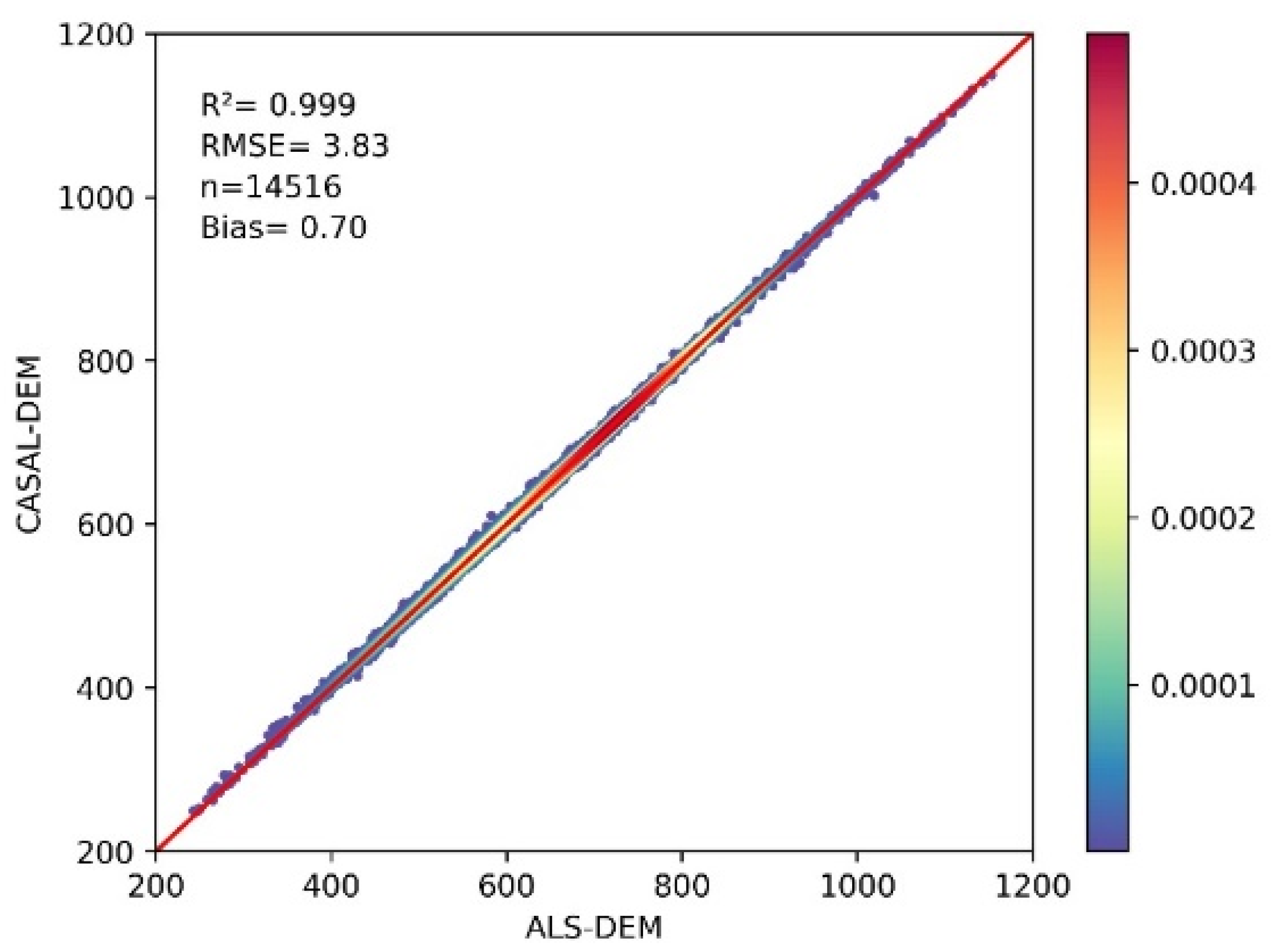
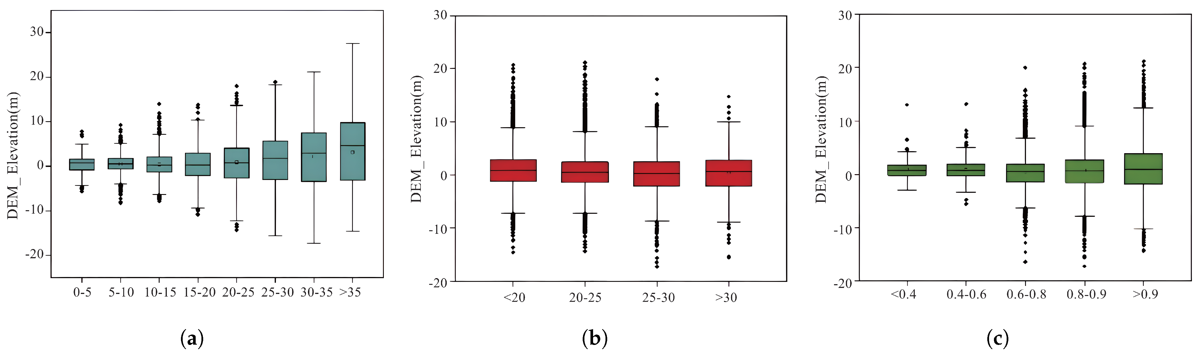
The study results demonstrate an exceptionally strong correlation ($R^2=0.999$) between CASAL-derived ground elevations and airborne light detection and ranging (LiDAR) DTM products. This high correlation confirms CASAL’s reliability for ground elevation inversion, particularly in flat or low-slope terrain. However, CASAL-DTM accuracy shows greater sensitivity to slope than to vegetation cover or tree height. This phenomenon likely results from reduced laser pulse penetration on steep slopes, increasing terrain inversion errors. Thus, CASAL applications in complex terrain may require correction through integration with additional data sources or algorithms. The median DTM difference (0.57 m) aligns with findings from comparable studies. For instance, Adam et al. [15] reported GEDI median DTM differences of −0.26 m and 0.18 m in Thuringia, suggesting systematic sensor-specific biases in topographic elevation inversion. Wang et al. [42] noted significant GEDI DTM variations across land cover and forest types, likely attributable to vegetation-specific laser pulse reflection and penetration characteristics. These findings corroborate previous GEDI topographic accuracy studies, further validating LiDAR data inversion performance variations across land cover types. CASAL-DTM exhibits minor topographic elevation overestimation compared to ALS-DTM, though within a smaller magnitude. Specifically, CASAL-DTM demonstrates lower error metrics than GEDI, with mean square error (RMSE) = 3.83 m, Bias = 0.70 m, median = 0.57 m, and median absolute deviation (MAD) = 2.96 m. These results indicate CASAL’s high accuracy for topographic elevation inversion, particularly in forested regions. Compared to GEDI, CASAL demonstrates more stable elevation inversion performance, potentially due to higher point cloud density and optimized data processing algorithms. Furthermore, the strong agreement between CASAL and ALS-DTM elevation inversions underscores CASAL’s potential for forest terrain monitoring applications.

4.2. Canopy Height

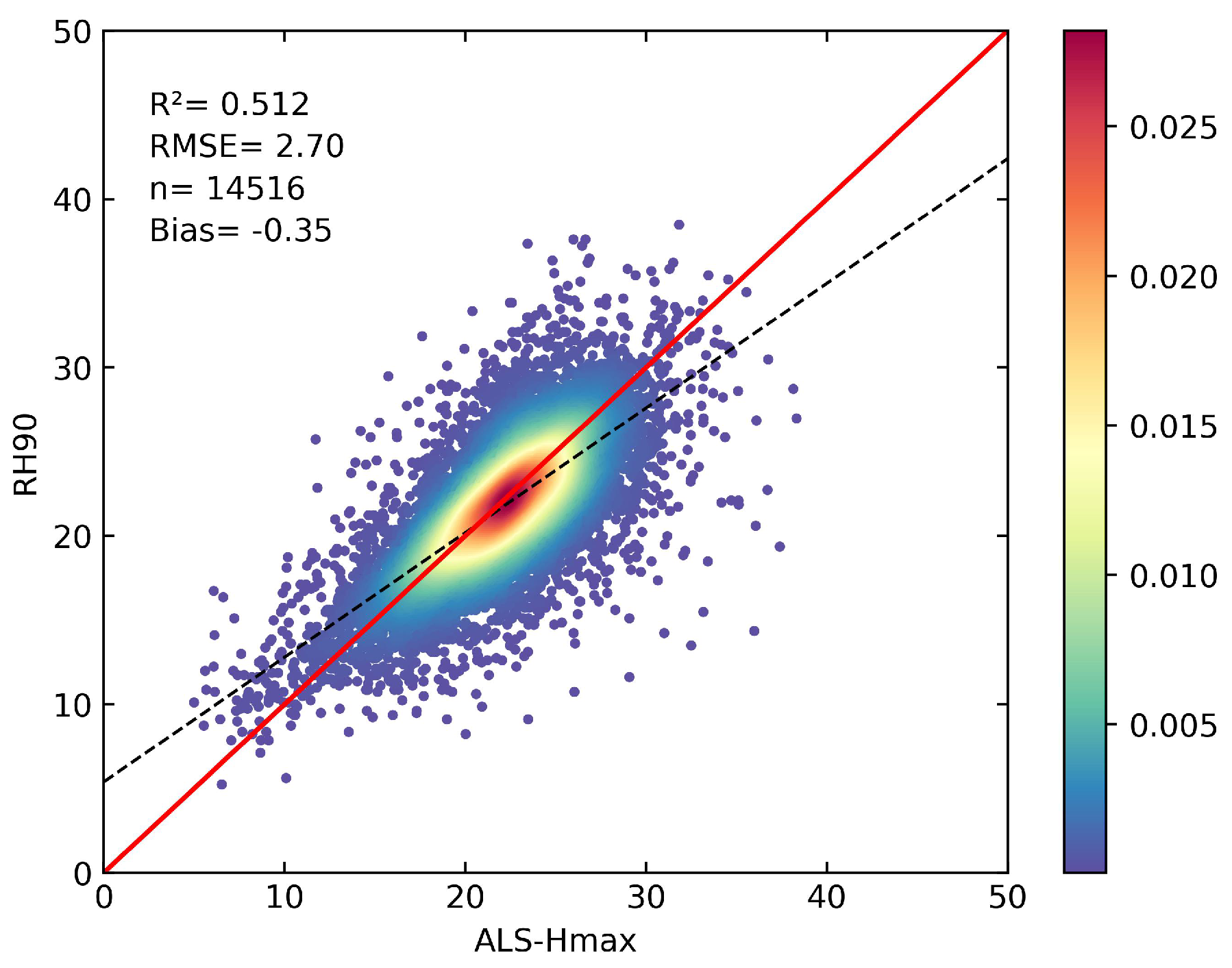
Among CASAL-derived relative height (RH) metrics, RH90 exhibited the strongest correlation with ALS-Hmax. This finding contrasts with Potapov and Zhu et al. [16,18], who identified GEDI’s RH95 as the optimal indicator of true forest height. This discrepancy likely arises from differences in pulse width between CASAL and GEDI systems. Furthermore, our results diverge from Liu et al.’s [39] findings. Their research demonstrated that ICESat-2’s RH98 most accurately represented true forest height. This inconsistency may result from temporal discrepancies between CASAL and ALS data acquisitions, which were not considered in our analysis. Additionally, their study incorporated diverse land cover types, potentially influencing results. These findings suggest that optimal height percentiles may vary across satellite systems depending on land cover characteristics.

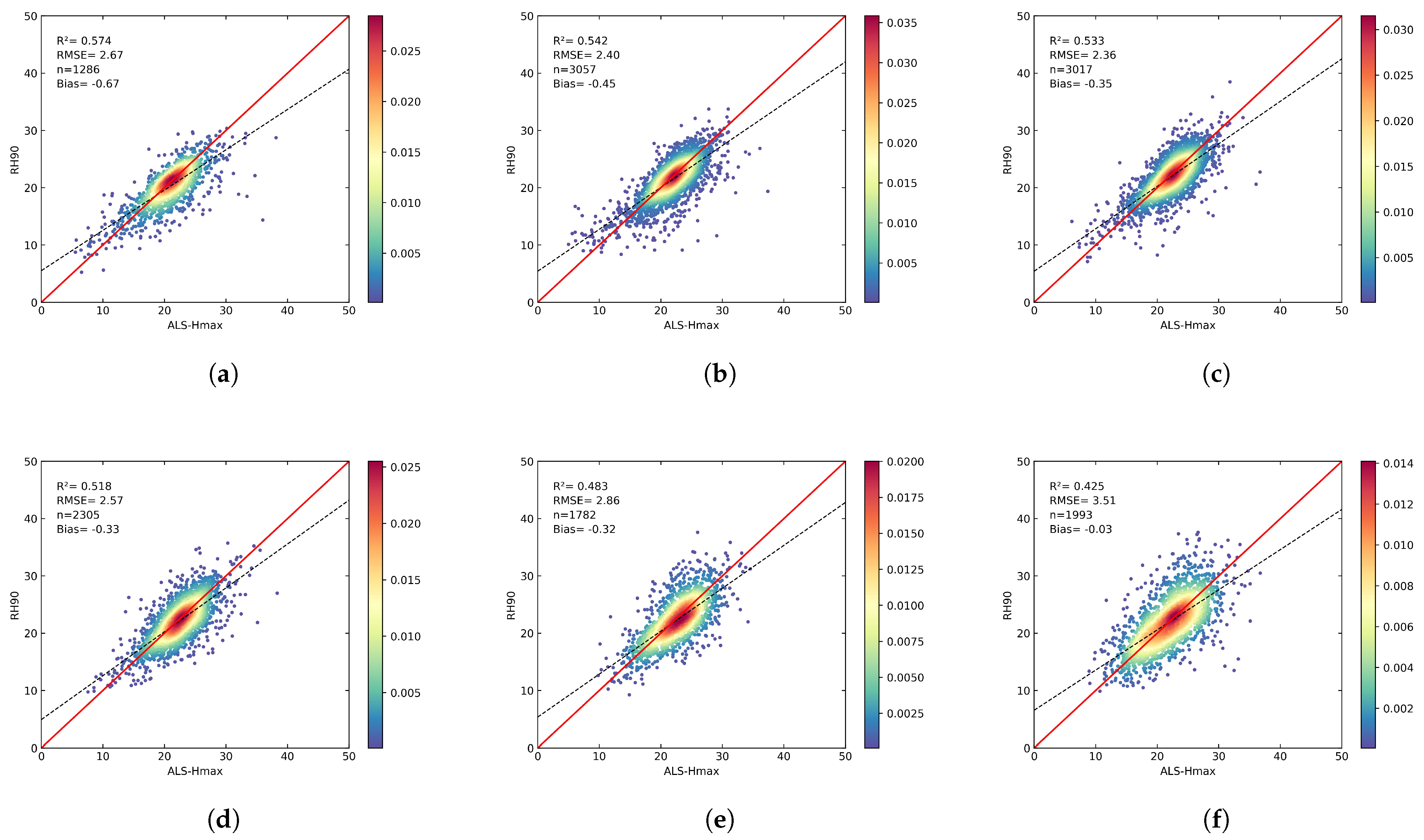
Steep terrain significantly contributes to CASAL waveform broadening and increased overlap between canopy and understory echoes. This broadening effect exacerbates waveform overlap, making CASAL-based canopy height estimation in high-slope areas particularly sensitive to terrain influence, thereby reducing estimation accuracy. Canopy height estimation accuracy ($R^2$, RMSE) declines with increasing slope. This occurs because waveform decomposition’s last peak reliably references canopy height in flat terrain, whereas slope-induced waveform broadening in non-flat areas reduces accuracy when using the last peak as a reference. As terrain slope increases, last-peak-based canopy height estimation becomes less accurate, explaining the observed inverse relationship between slope and estimation precision.

The forest canopy height estimation accuracy ($R^2$ and RMSE) in this study surpasses that reported by Chen et al. [43] for southwestern Quebec using CASAL parameters. This improvement is attributed to winter data collection, when reduced vegetation coverage enables CASAL laser pulses to penetrate forest stands more effectively, yielding precise understory topographic information. Enhanced penetration of CASAL laser pulses through winter canopies facilitates accurate differentiation between canopy and ground peaks, thereby improving canopy height estimation precision.

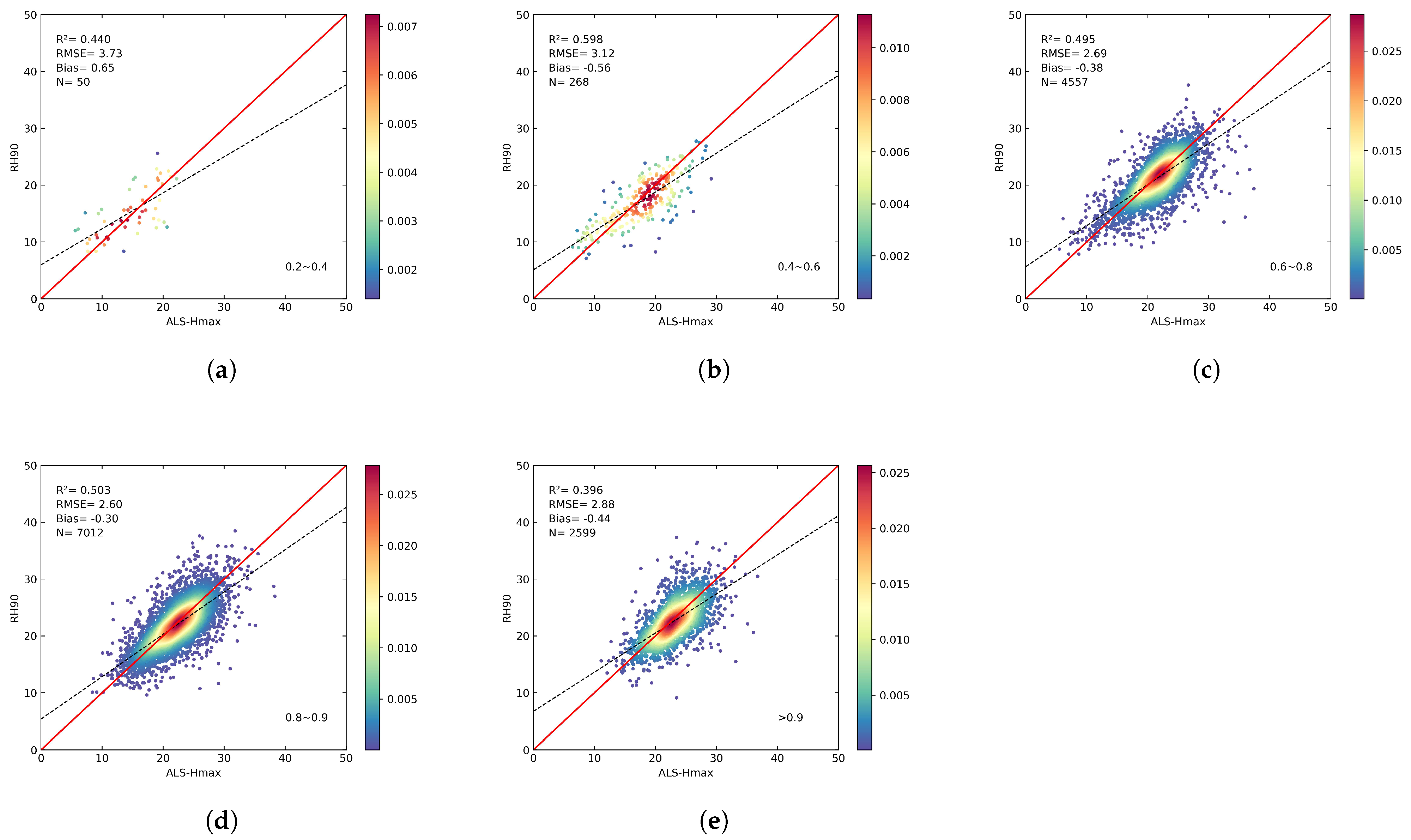
CASAL exhibits maximum canopy height inversion error at vegetation cover $>0.9$, likely due to limited laser pulse penetration through dense, structurally complex canopies, resulting in a misclassification of canopy echoes as ground returns. Conversely, in low-vegetation-cover areas, the highest waveform echo elevation may not correspond to the tallest canopy tree, potentially due to tree dispersion within the 25 m footprint and geolocation errors. The observed discrepancy between highest echo elevation and actual canopy height may result from tree dispersion within the 25 m footprint and geolocation inaccuracies.

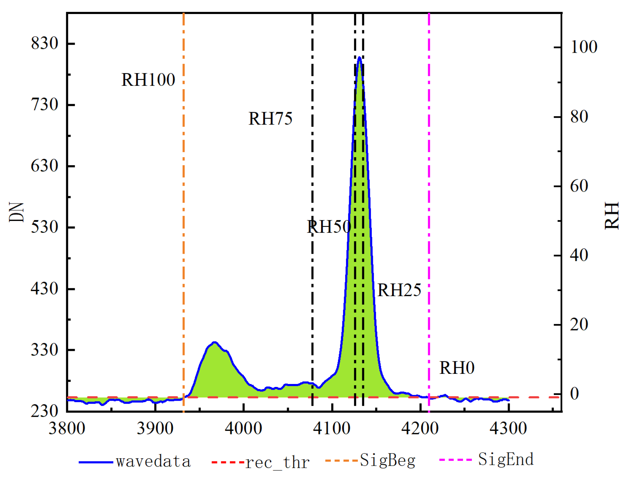
CASAL demonstrated optimal accuracy in mixed forests, evidenced by maximum $R^2$ values and minimum RMSE and MAD metrics. Broadleaf forests showed moderate accuracy, whereas coniferous forests exhibited the poorest performance among the three forest types. These performance variations likely stem from structural and canopy complexity differences among forest types, influencing system inversion efficacy.The study area contains extensive mixed and broadleaf forests. During winter leaf-off conditions, CASAL’s laser pulses effectively penetrate the canopy, enabling precise retrieval of subcanopy terrain information. Our findings demonstrate that winter leaf-off conditions in deciduous broadleaf forests significantly enhance the performance of spaceborne LiDAR canopy height retrievals. The improved signal penetration during winter is evidenced by the distinct separation of canopy and ground peaks in waveform data (Figure 4), enabling a more accurate identification of these features and consequently higher precision in forest canopy height estimation.

5. Conclusions

Using the Northeast Tiger and Leopard National Park as a study area, we systematically evaluated the terrain and canopy height inversion performance of the Carbon Sinks and Aerosol LiDAR (CASAL) system by comparing its L2 products with airborne LiDAR-derived data. Additionally, we validated the capabilities of next-generation satellite light detection and ranging (LiDAR) for detecting terrain elevation and forest canopy height changes. This study provides critical insights into the accuracy and potential of CASAL and satellite LiDAR technologies in ecological monitoring. Key findings include the following: (1) an exceptionally strong correlation ($R^2=0.999$) between CASAL-derived ground elevations and airborne laser scanning digital terrain model (DTM) products, with a root mean square error (RMSE) = 2.70 m and median DTM differences <0.7 m; (2) a significant linear relationship exists between canopy heights derived from terrestrial carbon monitoring satellite full-waveform data and airborne LiDAR measurements within footprint ranges. We further investigated relationships between multiple forest height metrics (RH80–RH100) and airborne LiDAR-derived forest heights. Our findings provide critical insights for applying terrestrial carbon monitoring satellite laser altimetry data to forest carbon stock estimation. Certain CASAL height estimation characteristics remain partially unexplained, potentially due to temporal data acquisition differences and forest vegetation growth dynamics. Future work should validate CASAL LiDAR performance across diverse environments and acquisition conditions, optimizing factors such as geolocation accuracy, reference data error reduction, and minimized data acquisition time differences.

References

1. Pugh, T.A.M.; Lindeskog, M.; Smith, B.; Poulter, B.; Arneth, A.; Haverd, V.; Calle, L. Role of Forest Regrowth in Global Carbon Sink Dynamics. Proc. Natl. Acad. Sci. USA 2019, 116, 4382–4387. [Google Scholar] [CrossRef] [PubMed]
2. Zhang, Z.; Cao, L.; She, G. Estimating Forest Structural Parameters Using Canopy Metrics Derived from Airborne LiDAR Data in Subtropical Forests. Remote Sens. 2017, 9, 940. [Google Scholar] [CrossRef]
3. Miura, N.; Jones, S.D. Characterizing Forest Ecological Structure Using Pulse Types and Heights of Airborne Laser Scanning. Remote Sens. Environ. 2010, 114, 1069–1076. [Google Scholar] [CrossRef]
4. Pasher, J.; King, D.J. Multivariate Forest Structure Modelling and Mapping Using High Resolution Airborne Imagery and Topographic Information. Remote Sens. Environ. 2010, 114, 1718–1732. [Google Scholar] [CrossRef]
5. Bryan Blair, J.; Hofton, M.A. Modeling Laser Altimeter Return Waveforms over Complex Vegetation Using High-Resolution Elevation Data. Geophys. Res. Lett. 1999, 26, 2509–2512. [Google Scholar] [CrossRef]
6. Goetz, S.; Dubayah, R. Advances in Remote Sensing Technology and Implications for Measuring and Monitoring Forest Carbon Stocks and Change. Carbon Manag. 2011, 2, 231–244. [Google Scholar] [CrossRef]
7. Gibbs, H.K.; Brown, S.; Niles, J.O.; Foley, J.A. Monitoring and Estimating Tropical Forest Carbon Stocks: Making REDD a Reality. Environ. Res. Lett. 2007, 2, 045023. [Google Scholar] [CrossRef]
8. Larjavaara, M.; Muller-Landau, H.C. Measuring Tree Height: A Quantitative Comparison of Two Common Field Methods in a Moist Tropical Forest. Methods Ecol. Evol. 2013, 4, 793–801. [Google Scholar] [CrossRef]
9. Asner, G.P.; Mascaro, J.; Muller-Landau, H.C.; Vieilledent, G.; Vaudry, R.; Rasamoelina, M.; Hall, J.S.; Van Breugel, M. A Universal Airborne LiDAR Approach for Tropical Forest Carbon Mapping. Oecologia 2012, 168, 1147–1160. [Google Scholar] [CrossRef]
10. Korhonen, L.; Korhonen, K.; Rautiainen, M.; Stenberg, P. Estimation of Forest Canopy Cover: A Comparison of Field Measurement Techniques. Silva Fenn. 2006, 40. [Google Scholar] [CrossRef]
11. Lefsky, M.A.; Cohen, W.B.; Parker, G.G.; Harding, D.J. Lidar Remote Sensing for Ecosystem Studies. Bioscience 2002, 52, 19. [Google Scholar] [CrossRef]
12. Simard, M.; Pinto, N.; Fisher, J.B.; Baccini, A. Mapping Forest Canopy Height Globally with Spaceborne Lidar. J. Geophys. Res. 2011, 116, G04021. [Google Scholar] [CrossRef]
13. Nie, S.; Wang, C.; Zeng, H.; Xi, X.; Xia, S. A Revised Terrain Correction Method for Forest Canopy Height Estimation Using ICESat/GLAS Data. ISPRS J. Photogramm. Remote Sens. 2015, 108, 183–190. [Google Scholar] [CrossRef]
14. Rajab Pourrahmati, M.; Baghdadi, N.; Fayad, I. Comparison of GEDI LiDAR Data Capability for Forest Canopy Height Estimation over Broadleaf and Needleleaf Forests. Remote Sens. 2023, 15, 1522. [Google Scholar] [CrossRef]
15. Adam, M.; Urbazaev, M.; Dubois, C.; Schmullius, C. Accuracy Assessment of GEDI Terrain Elevation and Canopy Height Estimates in European Temperate Forests: Influence of Environmental and Acquisition Parameters. Remote Sens. 2020, 12, 3948. [Google Scholar] [CrossRef]
16. Potapov, P.; Li, X.; Hernandez-Serna, A.; Tyukavina, A.; Hansen, M.C.; Kommareddy, A.; Pickens, A.; Turubanova, S.; Tang, H.; Silva, C.E.; et al. Mapping Global Forest Canopy Height through Integration of GEDI and Landsat Data. Remote Sens. Environ. 2021, 253, 112165. [Google Scholar] [CrossRef]
17. Selkowitz, D.J.; Green, G.; Peterson, B.; Wylie, B. A Multi-Sensor Lidar, Multi-Spectral and Multi-Angular Approach for Mapping Canopy Height in Boreal Forest Regions. Remote Sens. Environ. 2012, 121, 458–471. [Google Scholar] [CrossRef]
18. Zhu, X.; Nie, S.; Wang, C.; Xi, X.; Lao, J.; Li, D. Consistency Analysis of Forest Height Retrievals between GEDI and ICESat-2. Remote Sens. Environ. 2022, 281, 113244. [Google Scholar] [CrossRef]
19. Pang, Y.; Lefsky, M.; Sun, G.; Ranson, J. Impact of Footprint Diameter and Off-Nadir Pointing on the Precision of Canopy Height Estimates from Spaceborne Lidar. Remote Sens. Environ. 2011, 115, 2798–2809. [Google Scholar] [CrossRef]
20. Neuenschwander, A.L.; Magruder, L.A. Canopy and Terrain Height Retrievals with ICESat-2: A First Look. Remote Sens. 2019, 11, 1721. [Google Scholar] [CrossRef]
21. Brown, M.E.; Delgodo Arias, S.; Neumann, T.; Jasinski, M.F.; Posey, P.; Babonis, G.; Glenn, N.F.; Birkett, C.M.; Escobar, V.M.; Markus, T. Applications for ICESat-2 Data: From NASA’s Early Adopter Program. IEEE Geosci. Remote Sens. Mag. 2016, 4, 24–37. [Google Scholar] [CrossRef]
22. Magruder, L.A.; Brunt, K.M. Performance Analysis of Airborne Photon- Counting Lidar Data in Preparation for the ICESat-2 Mission. IEEE Trans. Geosci. Remote Sens. 2018, 56, 2911–2918. [Google Scholar] [CrossRef]
23. Markus, T.; Neumann, T.; Martino, A.; Abdalati, W.; Brunt, K.; Csatho, B.; Farrell, S.; Fricker, H.; Gardner, A.; Harding, D.; et al. The Ice, Cloud, and Land Elevation Satellite-2 (ICESat-2): Science Requirements, Concept, and Implementation. Remote Sens. Environ. 2017, 190, 260–273. [Google Scholar] [CrossRef]
24. Neuenschwander, A.; Guenther, E.; White, J.C.; Duncanson, L.; Montesano, P. Validation of ICESat-2 Terrain and Canopy Heights in Boreal Forests. Remote Sens. Environ. 2020, 251, 112110. [Google Scholar] [CrossRef]
25. Yu, J.; Nie, S.; Liu, W.; Zhu, X.; Lu, D.; Wu, W.; Sun, Y. Accuracy Assessment of ICESat-2 Ground Elevation and Canopy Height Estimates in Mangroves. IEEE Geosci. Remote Sens. Lett. 2022, 19, 1–5. [Google Scholar] [CrossRef]
26. Dubayah, R.; Blair, J.B.; Goetz, S.; Fatoyinbo, L.; Hansen, M.; Healey, S.; Hofton, M.; Hurtt, G.; Kellner, J.; Luthcke, S.; et al. The Global Ecosystem Dynamics Investigation: High-Resolution Laser Ranging of the Earth’s Forests and Topography. Sci. Remote Sens. 2020, 1, 100002. [Google Scholar] [CrossRef]
27. Chen, X.; Long, X.; Li, Q.; Li, J.; Han, Q.; Xu, Z.; Yao, W. Laser Data Processing and Accuracy Verification of the Terrestrial Ecosystem Carbon Monitoring Satellite. Geomat. Inf. Sci. Wuhan Univ. 2023, 1–18. [Google Scholar] [CrossRef]
28. Cao, H.; Zhang, X.; Qiu, X.; Huang, J.; He, T. Surveying Mountains and Rivers, Guarding the Skies—The Terrestrial Ecosystem Carbon Monitoring Satellite “Goumang”. Pop. Sci. Cult. Nat. Resour. 2023, 2, 14–21. [Google Scholar]
29. Pang, Y.; Li, Z.; Yu, T.; Liu, Q.; Zhao, L.; Chen, E. Current Status and Trends of Remote Sensing Satellites for Forest Carbon Storage. Spacecr. Recovery Remote Sens. 2022, 43, 1–15. [Google Scholar]
30. Wang, X.; Lü, Z.; Li, J.; Gong, Y.; Chen, W.; Lin, J. The Terrestrial Ecosystem Carbon Monitoring Satellite “Goumang” and Its Applications. Satell. Appl. 2023, 7, 18–22. [Google Scholar]
31. Pang, Y.; Yu, T.; Jia, W.; Liang, X.; Li, Z.; Fu, A.; Wu, F.; Liu, X.; Zhang, X.; Huang, J.; et al. TECIS: The First Mission Towards Forest Carbon Mapping by Combination Of Lidar And Multi-Angle Optical Observations. In Proceedings of the IGARSS 2023—2023 IEEE International Geoscience and Remote Sensing Symposium, Pasadena, CA, USA, 16–21 July 2023; pp. 1890–1893. [Google Scholar]
32. Fayad, I.; Baghdadi, N.; Bailly, J.S.; Frappart, F.; Zribi, M. Analysis of GEDI Elevation Data Accuracy for Inland Waterbodies Altimetry. Remote Sens. 2020, 12, 2714. [Google Scholar] [CrossRef]
33. Wang, X.; Huang, H.; Gong, P.; Liu, C.; Li, C.; Li, W. Forest Canopy Height Extraction in Rugged Areas with ICESat/GLAS Data. IEEE Trans. Geosci. Remote Sens. 2014, 52, 4650–4657. [Google Scholar] [CrossRef]
34. Lee, S.; Ni-Meister, W.; Yang, W.; Chen, Q. Physically Based Vertical Vegetation Structure Retrieval from ICESat Data: Validation Using LVIS in White Mountain National Forest, New Hampshire, USA. Remote Sens. Environ. 2011, 115, 2776–2785. [Google Scholar] [CrossRef]
35. Chen, Q. Retrieving Vegetation Height of Forests and Woodlands over Mountainous Areas in the Pacific Coast Region Using Satellite Laser Altimetry. Remote Sens. Environ. 2010, 114, 1610–1627. [Google Scholar] [CrossRef]
36. Fayad, I.; Baghdadi, N.N.; Alvares, C.A.; Stape, J.L.; Bailly, J.S.; Scolforo, H.F.; Zribi, M.; Maire, G.L. Assessment of GEDI’s LiDAR Data for the Estimation of Canopy Heights and Wood Volume of Eucalyptus Plantations in Brazil. IEEE J. Sel. Top. Appl. Earth Obs. Remote Sens. 2021, 14, 7095–7110. [Google Scholar] [CrossRef]
37. Hofton, M.; Blair, J.B.; Story, S. Algorithm Theoretical Basis Document (ATBD) for GEDI Transmit and Receive Waveform Processing for L1 and L2 Products (GEDI ATBD, Version 1.0). Available online: https://lpdaac.usgs.gov/documents/579/GEDI__WFGEO_ATBD_v1.0.pdf (accessed on 20 August 2022).
38. Hilbert, C.; Schmullius, C. Influence of Surface Topography on ICESat/GLAS Forest Height Estimation and Waveform Shape. Remote Sens. 2012, 4, 2210–2235. [Google Scholar] [CrossRef]
39. Liu, A.; Cheng, X.; Chen, Z. Performance Evaluation of GEDI and ICESat-2 Laser Altimeter Data for Terrain and Canopy Height Retrievals. Remote Sens. Environ. 2021, 264, 112571. [Google Scholar] [CrossRef]
40. Lahssini, K.; Baghdadi, N.; Le Maire, G.; Fayad, I. Influence of GEDI Acquisition and Processing Parameters on Canopy Height Estimates over Tropical Forests. Remote Sens. 2022, 14, 6264. [Google Scholar] [CrossRef]
41. Wang, C.; Zhu, X.; Nie, S.; Xi, X.; Li, D.; Zheng, W.; Chen, S. Ground Elevation Accuracy Verification of ICESat-2 Data: A Case Study in Alaska, USA. Opt. Express 2019, 27, 38168. [Google Scholar] [CrossRef]
42. Wang, C.; Elmore, A.J.; Numata, I.; Cochrane, M.A.; Shaogang, L.; Huang, J.; Zhao, Y.; Li, Y. Factors Affecting Relative Height and Ground Elevation Estimations of GEDI among Forest Types across the Conterminous USA. GISci. Remote Sens. 2022, 59, 975–999. [Google Scholar] [CrossRef]
43. Chen, J.; Li, G.; Peng, J.; Liu, Z.; Zhou, X. Accuracy Analysis of Forest Canopy Height from Waveform LiDAR of Terrestrial Ecosystem Carbon Inventory satellite (TECIS): A Case Study of Temperate Coniferous-Broadleaved Mixed Forest in Quebec, Canada. Natl. Remote Sens. Bull. 2024, 1–21. [Google Scholar] [CrossRef]
Figure 1. Cross-track relationships of CASAL lasers and distributions of ground tracks.
Applsci 15 06824 g001
Figure 2. Study area and distribution of LiDAR footprints. (a) Map showing the location of the study area within China (left) and a detailed view of the study region (right). (b) Spatial distribution of CASAL footprints across the study area.
Applsci 15 06824 g002
Figure 3. Workflow for accuracy assessment of CASAL products using airborne laser scanning (ALS) data.
Applsci 15 06824 g003
Figure 4. Characteristic full-waveform LiDAR return from the CASAL system. Typical waveforms and RH metrics for CASAL on relatively flat terrain. On flat terrain, the first Gaussian corresponds to reflections from the top of the canopy, while the last Gaussian refers mainly to the lowest point in the footprint, i.e., the ground.
Applsci 15 06824 g004
Figure 5. Example of point cloud representations within a footprint. (a,b) Spatial distribution of point clouds in the forested footprint area (ground points in red; canopy top points in green). (c) Point cloud data cropped to match the TECIS footprint dimensions and position.
Applsci 15 06824 g005
Figure 6. Comparison of CASAL elevation estimates with ALS-derived DTM.
Applsci 15 06824 g006
Figure 7. Differences between CASAL and ALS ground elevations by (a) slope, (b) vegetation height, and (c) cover.
Applsci 15 06824 g007
Figure 8. Validation of spaceborne CASAL RH90 against airborne ALS canopy height metrics. Scatter plot comparing canopy height estimates between the spaceborne CASAL system (RH90 metric) and airborne LiDAR (ALS Hmax) across 14,516 footprints. The least-squares regression line (black) and 1:1 reference line (red) are superimposed for comparative analysis.
Applsci 15 06824 g008
Figure 9. Scatter plots comparing CASAL-RH90 and ALS-Hmax canopy height estimates across six different categories of slope categories: (a) 0–5°, (b) 5–10°, (c) 10–15°, (d) 15–20°, (e) 20–25°, and (f) >25°. The least-squares regression line (black) and 1:1 reference line (red) are superimposed for comparative analysis.
Applsci 15 06824 g009
Figure 10. Scatter plots comparing CASAL-RH90 and ALS-Hmax canopy height estimates across five different categories of vegetation cover: (a) 0.2–0.4, (b) 0.4–0.6, (c) 0.6–0.8, (d) 0.8–0.9, and (e) >0.9. The least-squares regression line (black) and 1:1 reference line (red) are superimposed for comparative analysis.
Applsci 15 06824 g010