Hash-Guided Adaptive Matching and Progressive Multi-Scale Aggregation for Reference-Based Image Super-Resolution

Abstract

Reference-based super-resolution (RefSR) enhances the detail restoration capability of low-resolution images (LR) by utilizing the details and texture information of external reference images (Ref). This study proposes a RefSR method based on hash adaptive matching and progressive multi-scale dynamic aggregation to improve the super-resolution reconstruction capability. Firstly, to address the issue of feature matching, this chapter proposes a hash adaptive matching module. On the basis of similarity calculation between traditional LR images and Ref images, self-similarity information of LR images is added to assist in super-resolution reconstruction. By dividing the feature space into multiple hash buckets through spherical hashing, the matching range is narrowed down from global search to local neighborhoods, enabling efficient matching in more informative regions. This not only retains global modeling capabilities, but also significantly reduces computational costs. In addition, a learnable similarity scoring function has been designed to adaptively optimize the similarity score between LR images and Ref images, improving matching accuracy. Secondly, in the process of feature transfer, this chapter proposes a progressive multi-scale dynamic aggregation module. This module utilizes dynamic decoupling filters to simultaneously perceive texture information in both spatial and channel domains, extracting key information more accurately and effectively suppressing irrelevant texture interference. In addition, this module enhances the robustness of the model to large-scale biases by gradually adjusting features at different scales, ensuring the accuracy of texture transfer. The experimental results show that this method achieves superior super-resolution reconstruction performance on multiple benchmark datasets.

1. Introduction

The RefSR method significantly enhances the detail restoration of low-resolution (LR) images by introducing reference images (Ref) with similar content or texture. The core task of this method is to accurately match the detailed information between Ref and LR images, and effectively transfer the features of Ref images to LR images for super-resolution reconstruction.

Early RefSR methods, such as optical flow [1] and deformable convolution [2], mainly solved geometric differences between images through spatial alignment. The optical flow method relies on matching local pixels, while deformable convolution allows convolution operations to adaptively adjust based on local deformations. The SRNTT [3] method introduces a feature transformation module to optimize the relationships between images and improve the accuracy of detail restoration. The TTSR [4] method combines transformers and utilizes feature block matching to further enhance image detail restoration. MASA [5] adopts a coarse-to-fine matching strategy, ensuring good detail recovery while reducing computational complexity. C²-Matching [6] improves the accuracy of feature matching by combining knowledge extraction and contrastive learning, further enhancing detail recovery.

Although the existing RefSR methods have made some progress, the image block matching and pixel point matching strategies they adopt are limited to searching for the best texture transfer position in Ref images. However, rich and valuable texture information is not limited to a single location. Relying solely on a single match may result in insufficient transmission of texture information in Ref images, thereby affecting the final texture transfer effect. The root cause of this problem lies in the insufficient or even misuse of reference features, which limits the potential of matching strategies to improve the performance of RefSR methods.

The matching based the RefSR method often ignores the self-similarity of natural images, which has been widely applied and proven to be highly effective in SISR tasks. The self-similarity of an image refers to the repeated appearance of image blocks within the same image. Based on this characteristic, non-local sparse prior methods [7,8,9] have been extensively studied in the field of SISR, which can search for similar features globally and perform weighted fusion to enhance feature expression ability. In the RefSR task, as the Ref image typically contains multiple corresponding regions similar to the target LR image, and the LR image itself also has similar regions, these regions can provide richer information than a single matching point, thereby facilitating higher-quality super-resolution reconstruction.

To overcome these issues, we propose a RefSR method based on hash adaptive matching and progressive multi-scale dynamic aggregation. Firstly, to address the issue of feature matching, we introduced a hash adaptive matching module. By using spherical hashing to divide the feature space into multiple hash buckets, we limit the global search scope to local neighborhoods, significantly reducing computational costs. In addition, we designed a learnable similarity scoring function that adaptively optimizes the similarity score between LR and Ref images to ensure accurate matching.

Secondly, in the process of feature transfer, we propose a progressive multi-scale dynamic aggregation (PDA) module. This module uses a reference aware learnable filter to capture texture information in both spatial and channel domains, enabling more accurate extraction of image features. It prevents the inclusion of irrelevant textures and adaptively aggregates relevant texture information to ensure accurate texture transmission. In addition, gradually adjusting at each feature scale enhances the robustness of the model to large-scale biases.

In summary, the main contributions of this article are as follows:

• We propose a hash adaptive matching method that reduces the computational cost of global matching and improves matching accuracy between the LR and Ref images through adaptive similarity adjustment.
• We design dynamic filters that perceive texture information in both spatial and channel domains, optimizing the selection of Ref image features, reducing the introduction of irrelevant textures, and enhancing robustness to large-scale discrepancies through progressive adjustments.

2. Related Works

2.1. Single Image Super-Resolution

In 2014, SRCNN [10] was the first to apply deep learning techniques to super-resolution reconstruction, marking the rapid development of deep-learning-based super-resolution methods and their widespread adoption thereafter. The SISR method utilizes deep learning models to learn end-to-end mapping between LR and HR images, and its performance is significantly better than traditional algorithms [11,12,13]. Researchers have found that increasing the number of network layers can effectively expand the receptive field. Kim et al. [14] proposed the VDSR model, which further expands the receptive field by using a 20 layer deep network and accelerates the convergence of the network through residual connections, successfully alleviating the gradient explosion problem. Zhang et al. [15] proposed RCAN, which improves residual blocks by adding channel attention mechanism and is the first attention mechanism to be applied to each resolution image. In addition to improving the network structure to enhance super-resolution reconstruction performance, the selection of loss function is also an important factor in determining the quality of reconstructed images. Ledig et al. [16] proposed SRGAN, which uses a general adversarial network (GAN) [17] as the adversarial loss function to produce super-resolution results that are more in line with natural image distribution [18,19,20,21]. Recently, research has explored knowledge distillation frameworks [22,23] to further improve super-resolution performance.

2.2. Reference-Based Image Super-Resolution

Unlike traditional SISR methods, RefSR improves detail restoration by introducing additional high-resolution reference (Ref) images to reconstruct finer details. Reference images typically contain content related to LR images, providing authentic detail information for the reconstruction process. In 2018, Zheng et al. [1] proposed CrossNet, which aligns Ref and LR images through optical flow distortion. Although algorithms based on optical flow can alleviate the problem of image differences caused by multiple perspectives and scales, their computational complexity is high, and there are still bottlenecks in accurate optical flow prediction. To address this issue, Shim et al. [2] proposed a network structure called SSEN based on deformable convolution. The network adopts deformable convolution operation to construct feature association mapping between LR images and Ref images, and designs a dynamic offset estimation module to adaptively learn the deformation parameters of the convolution kernel. On the other hand, inspired by image style transfer, Zhang et al. [3] proposed an end-to-end deep learning model SRNTT, which restores LR images through neural texture transfer. This network performs dense block matching on image features and dynamically fuses the texture information of Ref images into LR images by analyzing the similarity of texture features, effectively filling the texture gaps in SR images. Yang et al. [4] pointed out that the SRNTT method ignores global information. They first introduced a transformer into RefSR and designed a TTSR model that mines deep feature correspondence relationships through attention mechanisms. In 2021, Lu et al. [5] proposed MASA, which uses a hierarchical enumeration matching scheme and a coarse to fine matching strategy to reduce computational overhead. However, due to the resolution difference between LR and Ref images, MASA still has limitations in repairing severely damaged textures, especially for non-local textures with low similarity, which typically provide more accurate detail information. In the same year, Jiang et al. [6] introduced C²-Matching, which combines knowledge extraction and contrastive learning to improve matching robustness and enhance feature alignment between LR and Ref images. In 2022, Li et al. [24] used wavelet transform to decompose image features into high-frequency and low-frequency sub-bands, further improving the efficiency of texture information transmission. In addition, Huang et al. [25] proposed a decoupling framework that divides the RefSR problem into two parts—super-resolution reconstruction and texture transfer—effectively alleviating issues related to insufficient or misused references. Zhang et al. [26] proposed a reciprocal learning framework that uses RefSR results as a new reference for the second RefSR and creates a feedback loop to improve performance. Zhang et al. [27] introduced the LMR framework, which integrates features from multiple reference images and constructs a large-scale super-resolution dataset. However, due to the size of the dataset, this is time-consuming. Zheng et al. [28] proposed MCM, a model that finds multiple corresponding points for each block or pixel in Ref images, utilizing more texture information and improving performance.

3. Our Approach

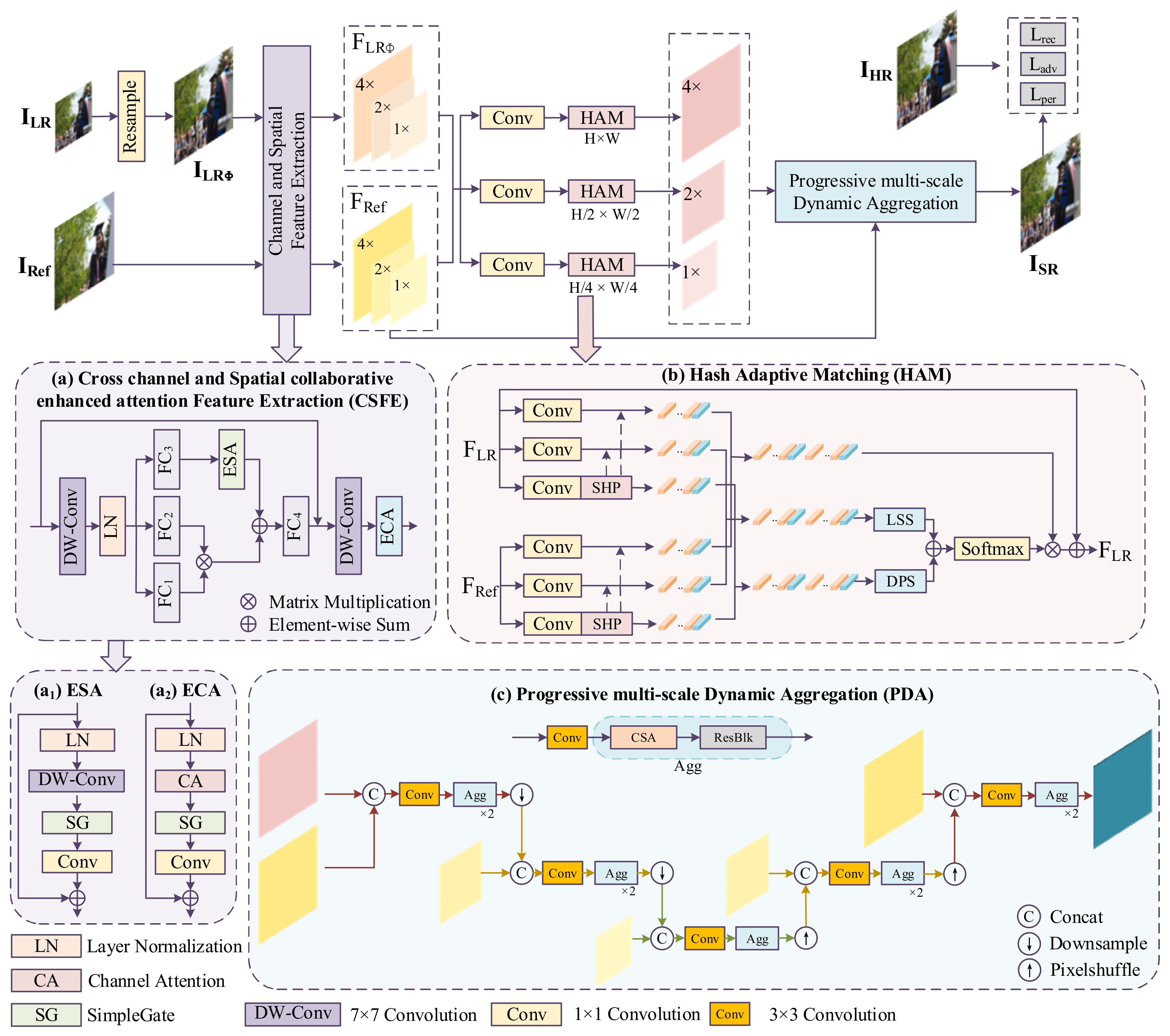
In this section, we first present the overall structure of the proposed method. We then introduce the cross-channel and spatial collaborative enhancement attention feature extraction module, the hash adaptive matching module, and the progressive multi-scale dynamic aggregation module.

3.1. Overall Framework

The overall framework of the proposed RefSR method is shown in Figure 1. The network inputs include the LR image I_LR and the Ref image I_Ref. We perform bilinear upsampling on the I_LR image to obtain I_LR↑. Both I_LR↑ and I_Ref are passed through the cross-channel and spatial collaborative enhancement attention feature extraction module, which extracts features at three scales: 1×, 2×, and 4×. The feature maps of the two images at corresponding scales are then paired together as inputs for subsequent hash adaptive matching and progressive multi-scale dynamic aggregation.

3.2. Channel Space Enhanced Attention Feature Extraction

The channel space enhanced attention feature extraction module (CSFE) consists of two depth-wise separable convolutions, four fully connected layers, a channel attention block, and a spatial attention block. First, the input features $F_{in}$ undergo a 7 × 7 depth-wise separable convolution to extract local features. Then, layer normalization is applied to obtain normalized features $F_i$. The normalized features $F_i$ are passed to three parallel fully connected layers. The output of the first fully connected layer $F{C}_1$ is passed through an activation function $ReLU6$, while the output of the third fully connected layer $F{C}_3$ is processed by the spatial attention block (ESA). The output of the second fully connected layer $F{C}_2$ is multiplied by the output of $F{C}_1$, and the result is added to the features processed by ESA to obtain the fused features. The fused features are then passed to the fourth fully connected layer $F{C}_4$ for further processing. Afterward, the processed features $F{C}_4$ undergo a second depth-wise separable convolution to extract additional features. Finally, the channel attention block (ECA) is applied to the features to obtain the final output features. A residual connection adds the input features $F_{in}$ directly to the features before the second depth-wise separable convolution layer, which helps alleviate the gradient vanishing problem and enhances feature learning.

3.3. Hash Adaptive Matching Module

Inspired by SISR self-similarity technology [29], we introduce self-similarity information within LR images based on the similarity calculation between LR images and Ref images. By combining the similarities within and between images, a hash adaptive matching (HAM) method is proposed to enhance the accuracy of matching, thereby more effectively guiding the super-resolution reconstruction process and achieving higher-quality image detail restoration.

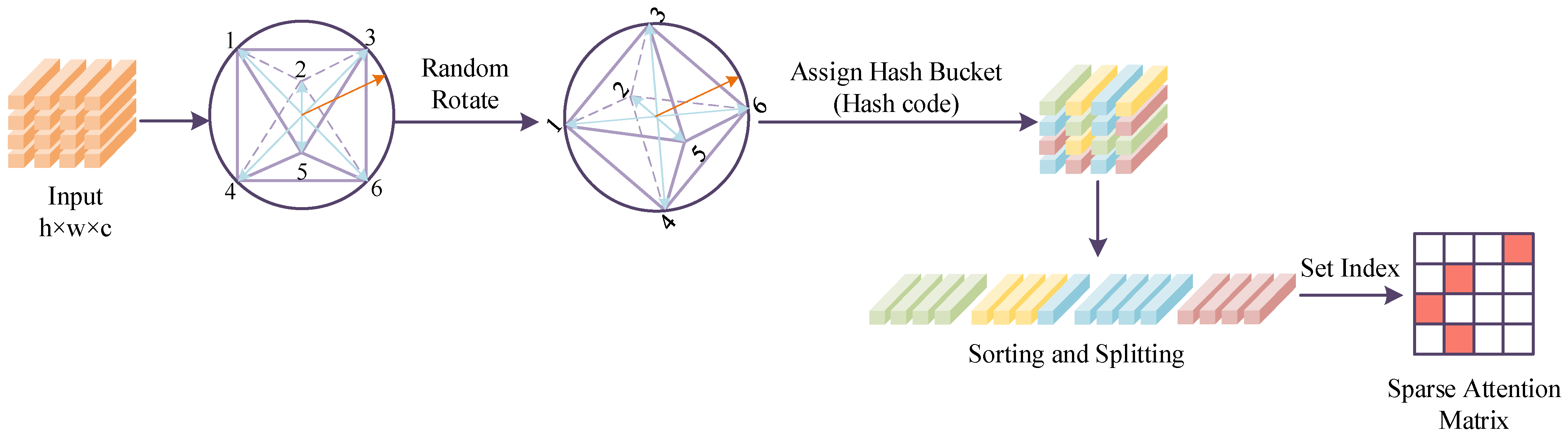
In order to facilitate the calculation of global attention, the features of the input LR and Ref images $F_{LR}=R^{h\times w\times c}$ and $F_{Ref}=R^{h\times w\times c}$ are first reshaped into one-dimensional feature vectors $F_{LR}^{\prime }=R^{hw\times c}$ and $F_{Ref}^{\prime }=R^{hw\times c}$. The traditional non-local attention mechanism requires a similarity calculation between all feature vectors pair-wise, which is computationally intensive. To reduce the complexity of this process, the HAM method uses the spherical hash partition (SHP) strategy [30]. This strategy divides the feature space based on the angular distance relationship between features, aggregates similar features into the same hash bucket, and performs attention calculation only in locally relevant regions.

Specifically, as shown in Figure 2, the basic idea of SHP is to nest a polyhedral structure within a unit sphere, use a hash function to map the eigenvectors to the outer surface of the sphere, and randomly rotate the polyhedral structure to ensure that the mapping process has sufficient randomness and directional coverage. Each feature vector selects the nearest vertex as its final hash index based on its angle with the vertices of the polyhedron. If the directions of two feature vectors are similar, that is, the angle between them is small, then they will be classified into the same hash bucket and identified as highly correlated features. Among them, the random rotation matrix has independent and identically distributed Gaussian components, ensuring the independence and uniformity of each hash mapping process in terms of direction.

To obtain m hash buckets, we must first project the target tensor onto a hypersphere and randomly rotate it using a matrix. The process of random rotation is as follows:

$$\widehat{x}=R({{\displaystyle \frac{x}{‖x‖}}}_2),$$

(1)

Here, $R$ is a size matrix c × m, c represents the dimension of input features, and m represents the number of hash buckets. Each element is an independent Gaussian variable N (0,1) sampled from below. This matrix is used to randomly project input features and is not strictly a rotation matrix. Map the feature vector x onto the sphere to obtain x′.

The hash computation process is as follows:

$$h(x)=\arg {\max }_i(\widehat{x}),$$

(2)

The hash code is defined as $h(x)$. After performing hash computation on all feature tensors, obtain multiple hash buckets, we need to divide the space into buckets of related elements, so we calculate the similarity within each bucket. ${\delta }_i$ represents the index of the bucket:

$${\delta }_i=\left\{h(x_j)=h(x_i)\right\},$$

(3)

Here, $i$ represents each feature tensor, ${\delta }_i$ is the index, and $j$ denotes the global feature.

The hash results are sorted and partitioned into blocks, each containing a fixed number of feature tensors, with an attention range defined for each block. The attention mechanism extends beyond block boundaries to incorporate adjacent regions. To address the issue of relevant features being dispersed into different buckets, multiple independent hash operations are performed, and their results are aggregated to minimize the error probability.

The attention process of the feature vector within the LR image, as well as between the LR and Ref images, can be expressed as follows:

$$HAM(x_i)={\displaystyle \sum _{x_j\in {\delta }_i}\frac{\exp (s(x_i,x_j))}{{\displaystyle {\sum }_{x_k\in {\delta }_i}\exp (s(x_i,x_k))}}}{\varphi }_v(x_j),$$

(4)

where $x_j$ and $x_k$ represent the $j$ and $\mathrm{k}$ feature vectors on $R^{2hw\times c}$, respectively, ${\varphi }_v(\cdot )$ is a feature embedding layer, $F^{\prime }=concat\left[F_{LR}^{\prime },F_{Ref}^{\prime }\right]$. $s(\cdot ,\cdot )$ represents the similarity measure between the two feature vectors, can be expressed as follows:

$$s(x_i,x_j)=s_l(x_i)+s_f(x_i,x_j),$$

(5)

The learnable similarity scoring function $s_l(x_i)$ allows the model to flexibly learn the contextual relevance of feature vectors $x_i$, as well as the bias information in the specific feature space. This can be explicitly expressed as:

$$s_l(x_i)=W_2\sigma (W_1{\varphi }_l(x_i)+b_1)+b_2,$$

(6)

where ${\varphi }_l(x_i)$ is the feature embedding layer, $W_1$ and $W_2$ are the learnable linear transformation matrices, $b_1$ and $b_2$ are the corresponding bias vectors, and $\sigma (\cdot )$ is the ReLU activation function.

The fixed dot product similarity scoring function $s_f(x_i,x_j)$ directly computes the correlation between feature vectors using the dot product, and it can be expressed as:

$$s_f(x_i,x_j)={\varphi }_q{(x_i)}^T{\varphi }_k(x_j),$$

(7)

where ${\varphi }_q(\cdot )$ and ${\varphi }_k(\cdot )$ share the same feature embedding layer, which is used for feature mapping.

Finally, the HAM module achieves efficient cross-image matching by processing the global features of both the LR and Ref images. The overall operation is as follows:

$$\begin{array}{l}C{F}_{LR}=HAM{(\mathit{concat}(F_{LR},F_{Ref}))}_{LR}+F_{LR},\\ C{F}_{Ref}=HAM{(\mathit{concat}(F_{LR},F_{Ref}))}_{Ref}+F_{Ref},\end{array}$$

(8)

where $HAM{(\cdot )}_{LR}$ and $HAM{(\cdot )}_{Ref}$ represent the feature outputs of the LR and Ref images, respectively, after cross-image attention fusion.

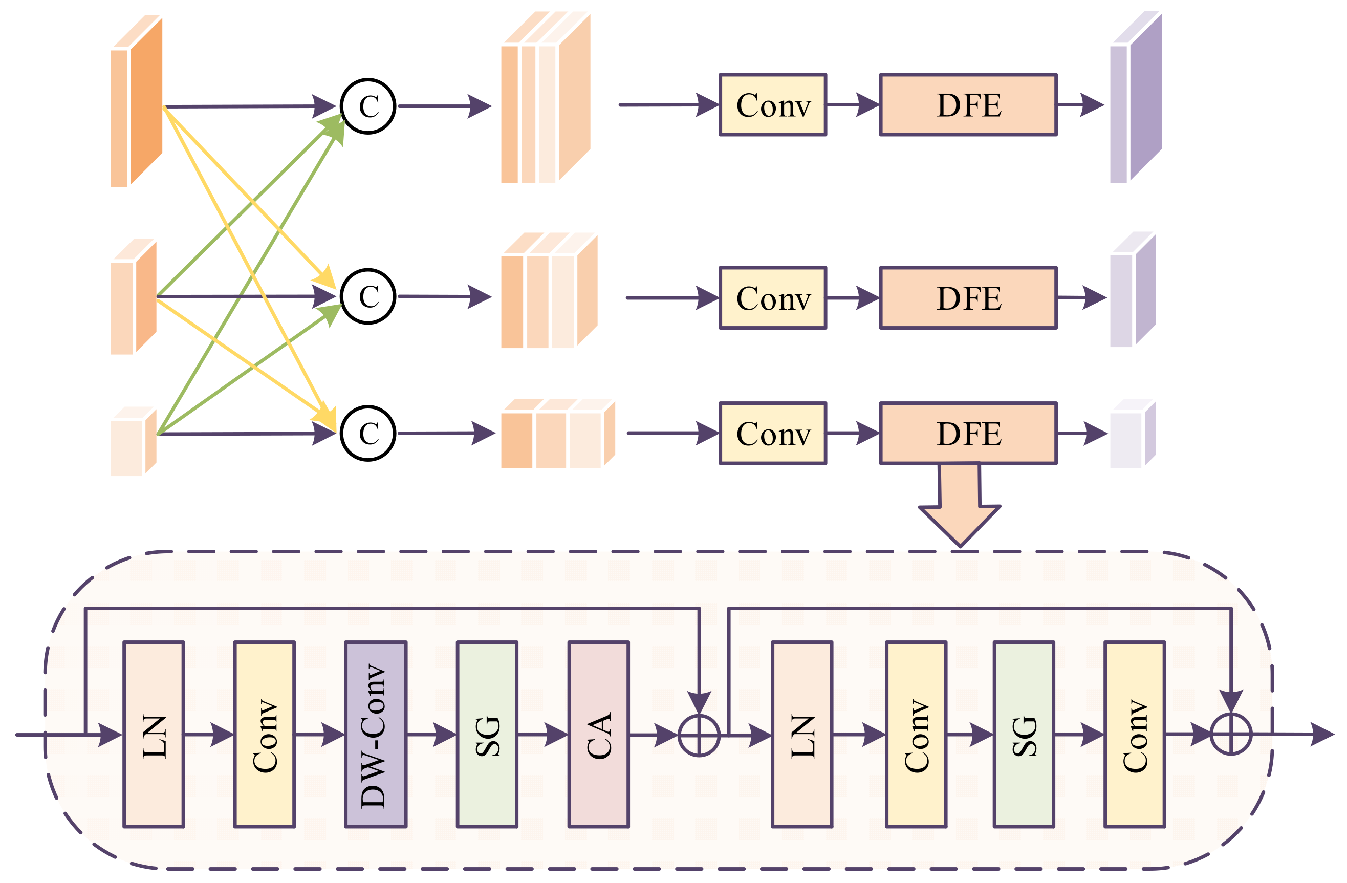
3.4. Progressive Multi-Scale Dynamic Aggregation

The LR images corresponding to each scale are fed into the multi-scale feature interaction (MSI) module to facilitate cross-scale feature interaction, thereby further enhancing and integrating the feature representations, as shown in Figure 3.

The features of the second scale are upsampled once, and the features of the third scale are upsampled twice. These two features are then concatenated with the features from the first scale along the channel dimension. Afterward, a convolution operation is applied to reduce the number of channels to one-third, followed by a feature extraction module for further feature extraction.

The features of the first scale are downsampled once, and the features of the third scale are upsampled once. These two features are concatenated along the channel dimension with the features from the second scale. Then, a convolution operation is applied to reduce the number of channels to one-third, followed by feature extraction through the feature extraction module.

The features from the first scale are downsampled twice, and the features from the second scale are downsampled once. These two features are then concatenated along the channel dimension with the features from the third scale. Afterward, convolution is applied to compress the number of channels to one-third, followed by feature extraction using a feature extraction module.

After feature interaction through the MSI module, the LR image features at three scales are input into the PDA, where progressive dynamic aggregation is performed multiple times at each scale to complete the super-resolution reconstruction.

$$F_{Agg}=PDA(Conv([F_{LR};F_{Ref}]))+F_{LR},$$

(9)

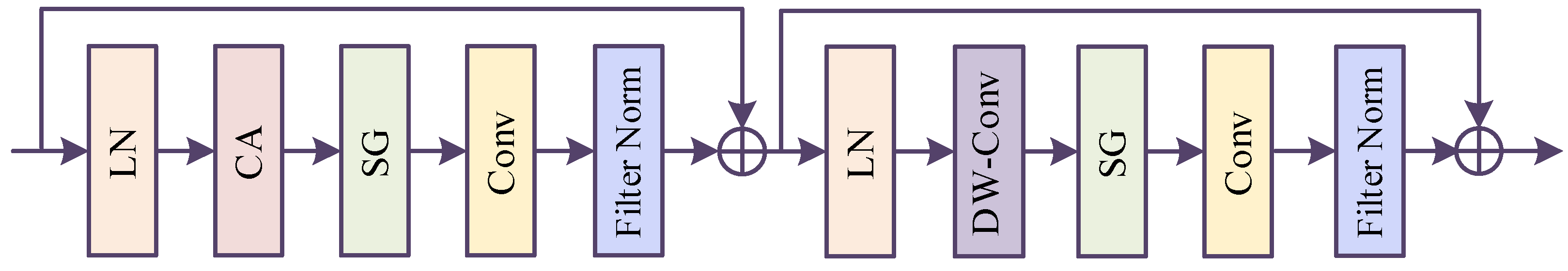
The aligned low-resolution (LR) image features are concatenated with the reference (Ref) image features, which are subsequently fed into a convolutional layer. A dynamic decoupling filter, namely the channel–spatial attention (CSA) mechanism, is then employed to extract texture information across both spatial and channel domains. The structure of CSA is shown in the Figure 4.

In the spatial domain, CSA extracts features through the spatial gate (SG) module and convolution. The SG module captures the local correlation between pixels and dynamically generates weights related to the texture, thereby enhancing the spatial feature representation of the image. Additionally, the convolution operation further refines the spatial domain features, ensuring that the texture details of local regions are fully preserved.

In the channel domain, CSA utilizes the channel attention (CA) module to adaptively adjust the weight distribution of channel features. CA models the importance of different channels and dynamically optimizes the feature representation ability, enabling efficient processing and expression of multi-channel features.

Following the channel-wise and spatial domain output operations, a filtering normalization process was implemented to standardize the feature representations.

$$\begin{array}{l}{N}_i^s={\alpha }^s{\displaystyle \frac{N_i^{\prime s}-\mu (N_i^{\prime s})}{\delta (N_i^{\prime s})}}+{\beta }^s,\\ N_k^c={\alpha }^c{\displaystyle \frac{N_k^{\prime c}-\mu (N_k^{\prime c})}{\delta (N_k^{\prime c})}}+{\beta }^c,\end{array}$$

(10)

where $N_i^{\prime s}$ and $N_k^{\prime c}$ represent the spatial and channel filters before filter normalization, respectively. $\mu (\cdot )$ and $\delta (\cdot )$ are used to compute the mean and standard deviation of the filters, while ${\alpha }^s$, ${\alpha }^c$, ${\beta }^s$, and ${\beta }^c$ are learnable scaling and shift parameters, similar in function to the scale and shift parameters in batch normalization [31], used to control the normalized numerical range. The four parameters are defined as 1 during network initialization and updated through backpropagation training of the entire network. The decoupled dynamic filtering operation can be expressed as:

$$F_{(k,i)}^{\prime }={\displaystyle \sum _{j\in \mathrm{\Omega }(i)}({N_i^s}_{(p_i-p_j)}}({N_k^c}_{(p_i-p_j)}))F_{(k,j)},$$

(11)

where $F_{(k,i)}^{\prime }$ represents the output feature value at the $i$-th pixel and k-th channel, and $F_{(k,j)}$ represents the input feature value at the $j$-th pixel and $\mathrm{k}$-th channel. $\mathrm{\Omega }(i)$ represents the set of pixels within the convolution window centered on pixel $i$-th, using a fixed size 3 × 3 convolution. $N_k^c$ represents the channel filter, generated by channel attention, calculates dynamic weights based on relative position (distance difference between pixels). This weight is used to control which spatial regions contribute more to the current pixel. For example, if the distance between one pixel and another is close and the spatial attention value is high, then it indicates that these two pixels have a higher correlation in computation. $N_i^s$ represents the spatial filter, a dynamic weight generated by the spatial gate, used to control the importance of different channels. By learning the weights of each channel, the model can automatically adjust the weights between channels based on the specific requirements of input features. $p_i$ and $p_j$ represent the spatial coordinates of the pixels, and $p_i-p_j$ is used to calculate the relative position between two pixels. This formula represents that for the $\mathrm{k}$-th channel and the $i$-th pixel, the decoupled dynamic filter weights the pixel contributions within its neighborhood $\mathrm{\Omega }(i)$ based on channel attention and spatial attention to complete feature reconstruction.

Finally, the features after decoupled dynamic filtering are passed through the ResBlock to achieve dynamic aggregation.

3.5. Loss Function

Reconstruction loss: The ${\mathcal{L}}_1$ norm was employed as the reconstruction loss function:

$${\mathcal{L}}_{rec}=\left|\right|I^{HR}-I^{SR}|{|}_1,$$

(12)

where $I^{HR}$ and $I^{SR}$ represent the ground truth image and the reconstructed output.

Perceptual loss: The perceptual loss [32] is used to improve visual quality:

$${\mathcal{L}}_{per}={\displaystyle \frac{1}{V}}{\displaystyle \sum _{i=1}^C\left|\right|{\varphi }_i(I^{HR})-{\varphi }_i(I^{SR})|{|}_F},$$

(13)

where $V$ and $C$ represent the volume and number of channels of the feature maps, $\varphi$ represent the relu5_1 features of the VGG19 [33] model, and $\left|\right|\cdot |{|}_F$ denotes the Frobenius norm.

Adversarial loss: The adversarial loss [16] is defined as follows:

$${\mathcal{L}}_{adv}=-D(I^{SR}),$$

(14)

The loss function for training the discriminator $D$ is defined as follows:

$${\mathcal{L}}_D=D(I^{SR})-D(I^{HR})+\lambda \left|\right|{\nabla }_{\widehat{i}}D(\widehat{I})|{|}_2-1{)}^2,$$

(15)

where $\widehat{I}$ is a random convex combination of $I^{SR}$ and $I^{HR}$.

The overall loss of the model is finally:

$$\mathcal{L}={\lambda }_{rec}{\mathcal{L}}_{rec}+{\lambda }_{per}{\mathcal{L}}_{per}+{\lambda }_{adv}{\mathcal{L}}_{adv},$$

(16)

4. Experiments

4.1. Datasets

Training dataset: We use the CUFED [3] dataset’s training set to train our model. The training set contains 11,871 pairs of input and reference images, with each image having a resolution of 160 × 160. It includes diverse scenes like people, buildings, and landscapes, helping the model learn rich features.

Testing dataset: We evaluated the performance on several datasets, including the CUFED5 [3], Sun80 [34], Urban100 [35], Manga109 [36], and WR-SR [6] datasets. Specifically, CUFED5 is the test set of CUFED, with 126 input images and 5 reference images per input at different similarity levels. It helps evaluate how well the model handles varying similarity, especially low-similarity regions. The Sun80 dataset consists of 80 images, each paired with one reference image selected from 20 web-searched candidates. It tests the model’s ability to select and use the most suitable reference in a multi-reference setting. The Urban100 dataset contains 100 images of urban scenes with strong lines and geometric structures. It uses the image itself as the reference to assess the model’s ability to exploit internal self-similarity, particularly for complex textures and geometry. The Manga109 dataset includes 109 Japanese manga images. A random image from the dataset is used as the reference to evaluate how well the model handles content and structure unique to manga-style images. MR-SR is similar to CUFED5, but the LR and Ref images are paired one-to-one, with a total of 80 pairs of images. It is used to test the model’s basic reconstruction performance in practical scenarios.

Evaluation metrics: We use PSNR and SSIM on the Y channel of the YCbCr color space as evaluation metrics. The HR images are downsampled by a factor of 4 using bicubic interpolation to generate the input LR images for evaluation.

4.2. Experimental Details

The HR image is downsampled by a factor of 4 using bicubic interpolation to obtain the LR image for super-resolution reconstruction. To augment the training data, we applied horizontal flipping, vertical flipping, and random rotations of 90°, 180°, and 270°. During hash-based adaptive matching, we set the number of hash computations to 4, with each computation generating a different hash value through independent operations. The size of each hash bucket is set to 144. Matching is performed at three scales: 160 × 160, 80 × 80, and 40 × 40, thus utilizing the richness of multi-scale features. The progressive adaptive aggregation module performs progressive aggregation in a large-medium-small-medium-large scale order, with each scale being aggregated twice except for the smallest scale, which is aggregated once. By gradually refining and alternately enhancing local and global information, it is possible to restore image details while maintaining the global consistency and structural integrity of the image. During training, we optimize the model using the Adam optimizer, setting the parameters ${\beta }_1$ and ${\beta }_2$ to 0.99 and 0.999, respectively. The initial learning rate is set to 1e⁻⁴, and the batch size is 9. Each batch contains 9 LR patches of size 40 × 40 and 9 reference patches of size 160 × 160. We use ${\mathcal{L}}_{adv}$ as the sole loss function, with joint supervision from ${\mathcal{L}}_{rec}$, ${\mathcal{L}}_{per}$, and ${\mathcal{L}}_{adv}$. The weights for ${\mathcal{L}}_{rec}$, ${\mathcal{L}}_{per}$, and ${\mathcal{L}}_{adv}$ are set to 1.0, 10⁻⁴, and 10⁻⁶, respectively. ${\mathcal{L}}_{rec}$ (1.0) is the main loss, ensuring the output closely matches the ground truth at the pixel level and provides stable training. ${\mathcal{L}}_{per}$ (10⁻⁴) improves visual quality by comparing high-level features from a pretrained network. A small weight prevents it from overpowering the training. ${\mathcal{L}}_{adv}$ (10⁻⁶) helps make the output more realistic. Due to its instability, it is given a very low weight to avoid disrupting training. The model is implemented in PyTorch 1.13.1 and trained on an NVIDIA 3090 GPU (NVIDIA, Santa Clara, CA, USA).

4.3. Comparison with State-of-the-Art Methods

We perform both quantitative and qualitative comparisons between our proposed method and several existing SISR and RefSR methods. The SISR methods include SRCNN [10], EDSR [12], RCAN [15], SRGAN [16], Enet [37], ESRGAN [18], and RankSRGAN [19]. The RefSR methods include CrossNet [1], SRNTT [3], TTSR [4], SSEN [2], MASA [5], C²-Matching [6], and RRSR [26]. We train two sets of parameters: one using all loss functions and another using only the reconstruction loss (denoted as -rec).

4.3.1. Quantitative Comparison

As shown in

Table 1. Quantitative comparison between SISR model and RefSR model (using only reconstruction loss, suffix “-rec”). The best and second best PSNR/SSIM values are marked in bold and underlined in the table, respectively.

	Method	CUFED5 [3]	Sun80 [34]	Urban100 [35]	Manga109 [36]	WR-SR [6]
		PSNR/SSIM	PSNR/SSIM	PSNR/SSIM	PSNR/SSIM	PSNR/SSIM
SISR	SRCNN [10]	25.33/0.745	28.26/0.781	24.41/0.738	27.12/0.850	27.27/0.767
	EDSR [12]	25.93/0.777	28.52/0.792	25.51/0.783	28.93/0.891	28.07/0.793
	RCAN [15]	26.06/0.769	29.86/0.810	25.42/0.768	29.38/0.895	28.25/0.799
	SRGAN [16]	24.40/0.702	26.76/0.725	24.07/0.729	25.12/0.802	26.21/0.728
	Enet [37]	24.24/0.695	26.24/0.702	23.63/0.711	25.25/0.802	25.47/0.699
	ESRGAN [18]	21.90/0.633	24.18/0.651	20.91/0.620	25.53/0.797	26.07/0.726
	RankSRGAN [19]	22.31/0.635	25.60/0.667	21.47/0.624	25.04/0.803	26.15/0.719
RefSR	CrossNet [1]	25.48/0.764	28.52/0.793	25.11/0.764	23.36/0.741	23.77/0.612
	SRNTT-rec [3]	26.24/0.784	28.54/0.793	25.50/0.783	28.95/0.885	27.59/0.780
	TTSR-rec [4]	27.09/0.804	30.02/0.814	25.87/0.784	30.09/0.907	27.97/0.792
	SSEN-rec [2]	26.78/0.791	-	-	-	-
	MASA-rec [5]	27.54/0.814	30.15/0.815	26.09/0.786	30.28/0.909	28.19/0.796
	C2-Matching-rec [6]	28.24/0.841	30.18/0.817	26.03/0.785	30.47/0.911	28.32/0.801
	RRSR-rec [26]	28.83/0.856	30.13/0.816	26.21/0.790	30.91/0.913	28.41/0.804
	Ours-rec	28.62/0.853	30.25/0.819	26.29/0.793	31.02/0.915	28.49/0.802

, our method, using only the reconstruction loss, achieves state-of-the-art results on the three benchmark datasets: Sun80, Urban100, and Manga109. For the more complex datasets CUFED5 and WR-SR, our model also demonstrates exceptional generalization ability, outperforming most of the comparison methods and achieving better results than the baseline method C²-Matching. Our method leverages effective adaptive learnable texture matching and dynamic texture transfer during reconstruction, which allows similar textures from high-resolution reference images in the dataset to be transferred to low-resolution images, thereby enhancing high-frequency information. This adaptive transfer strategy effectively addresses the misalignment issue in texture transfer found in traditional methods, significantly improving detail restoration while maintaining structural consistency.

According to the results in

Table 2. Quantitative comparison between SISR model and RefSR model (using reconstruction loss, adversarial loss, perceptual loss). The best and second best PSNR/SSIM values are marked in bold and underlined in the table, respectively.

	Method	CUFED5 [3]	Sun80 [34]	Urban100 [35]	Manga109 [36]	WR-SR [6]
		PSNR/SSIM	PSNR/SSIM	PSNR/SSIM	PSNR/SSIM	PSNR/SSIM
SISR	SRCNN [10]	25.33/0.745	28.26/0.781	24.41/0.738	27.12/0.850	27.27/0.767
	EDSR [12]	25.93/0.777	28.52/0.792	25.51/0.783	28.93/0.891	28.07/0.793
	RCAN [15]	26.06/0.769	29.86/0.810	25.42/0.768	29.38/0.895	28.25/0.799
	SRGAN [16]	24.40/0.702	26.76/0.725	24.07/0.729	25.12/0.802	26.21/0.728
	Enet [37]	24.24/0.695	26.24/0.702	23.63/0.711	25.25/0.802	25.47/0.699
	ESRGAN [18]	21.90/0.633	24.18/0.651	20.91/0.620	25.53/0.797	26.07/0.726
	RankSRGAN [19]	22.31/0.635	25.60/0.667	21.47/0.624	25.04/0.803	26.15/0.719
RefSR	CrossNet [1]	25.48/0.764	28.52/0.793	25.11/0.764	23.36/0.741	23.77/0.612
	SRNTT [3]	25.61/0.764	27.59/0.756	25.09/0.774	27.54/0.862	26.53/0.745
	TTSR [4]	25.53/0.765	28.59/0.774	24.62/0.747	28.70/0.886	26.83/0.762
	SSEN [2]	25.35/0.742	-	-	-	-
	MASA [5]	24.92/0.729	27.12/0.708	23.78/0.712	27.34/0.848	25.76/0.717
	C2-Matching [6]	27.16/0.805	29.75/0.799	25.52/0.764	29.73/0.893	27.80/0.780
	RRSR [26]	28.09/0.835	29.57/0.793	25.68/0.767	29.82/0.893	27.89/0.784
	Ours	27.78/0.824	29.77/0.801	25.81/0.774	29.90/0.898	27.83/0.782

, after introducing perceptual loss and adversarial loss for joint supervision, our model still shows significant advantages. Despite the trade-off effect between different loss functions causing some fluctuation in quantitative metrics, our method remains superior in most comparison scenarios. Through quantitative comparisons under both paradigms, our architecture demonstrates excellent robustness. Its stable performance across different supervision modes verifies the versatility of the method’s design and achieves optimal performance.

4.3.2. Qualitative Evaluation

Figure 5 shows a visual comparison of our model with existing SISR and RefSR methods. We compared our method with several of the current top-performing methods, including ESRGAN [18], RankSRGAN [19], TTSR [4], MASA [5], C²-Matching [6], and RRSR [26]. It is evident from the figure that SISR methods struggle with severe degradation of high-frequency information in the LR images, and ESRGAN and RankSRGAN have difficulty reconstructing texture details, especially when dealing with text, faces, and fine textures. Compared to SISR, RefSR methods can transfer similar textures from reference images, thereby generating more texture details. In comparison with existing RefSR methods, our model, through its adaptive features, better perceives and transfers texture information from the reference image. As a result, our model effectively compensates for the missing high-frequency details in the low-resolution image, leading to texture reconstruction that is much closer to the real image. We have marked the areas of interest (i.e., enlarged details) with red boxes in the figure, and presented corresponding enlarged images for comparative analysis below.

For example, in the first group of images, regarding text information, ESRGAN and RankSRGAN methods failed to effectively restore clear text. Although the visualized images of other methods show some recognizable letters, there is still noticeable distortion. In contrast, our method is able to clearly and accurately restore the text information in the image, avoiding blurriness and loss of details, demonstrating a significant advantage.

Through six sets of comparison images, it is evident that our method outperforms existing RefSR methods in texture detail restoration, recovering more high-frequency information and fine details. This thoroughly demonstrates the effectiveness of our proposed adaptive texture matching and aggregation approach, which not only improves image quality but also enhances the realism of the reconstructed images.

5. Ablation Studies

This section conducted ablation experiments to evaluate the effectiveness of each module. As shown in

Table 3. Quantitative Evaluation of HAM and Agg on the CUFED Dataset.

Model	HAM	Agg	PSNR↑/SSIM↑
Baseline			26.66/0.789
Baseline + HAM	√		27.88/0.810
Baseline + HAM + Agg	√	√	28.62/0.853

, in order to more accurately measure the performance of the proposed module in texture regions, the CUFED 5 dataset was selected for the experiment. This dataset contains rich and complex texture information, which poses a high challenge and is more suitable for testing the texture aggregation ability of the model compared to other datasets. In the experimental process, this section starts by removing the Agg module from hash adaptive matching (HAM) and progressive multi-scale aggregation (PDA), and gradually introduces various ablation modules to analyze their impact on model performance. By gradually restoring different modules, it is possible to quantify the contribution of each module and verify its role in overall performance improvement.

5.1. Hash Adaptive Matching

5.1.1. Learnable Similarity Scoring

Table 4. Quantitative Evaluation of LSS.

Model	DPS	LSS	PSNR↑/SSIM↑
Baseline			26.66/0.789
Baseline + HAM (w/o LSS)	√		27.72/0.795
Baseline + HAM (w/ LSS)	√	√	27.88/0.810

shows the performance improvement of our proposed learnable similarity scoring function (LSS) compared to the traditional fixed dot product similarity scoring function (DPS) on the CUFED5 dataset. Specifically, the image super-resolution reconstruction results based on our method significantly outperform traditional approaches, effectively recovering more details and texture information.

Additionally, we conducted further evaluations on datasets such as Sun80, Urban100, and Manga109, with the results shown in Figure 6. By using the learnable similarity scoring function, which can dynamically adjust the attention to different feature vectors, the model becomes more flexible and precise when handling complex textures and details. Especially when dealing with images containing diverse textures and structures, our method is able to capture and recover important high-frequency details with greater accuracy, further enhancing image quality and visual effects. We have marked the areas of interest (i.e., enlarged details) with red boxes in the figure, and presented corresponding enlarged images for comparative analysis below.

5.1.2. Hash Rounds

As mentioned earlier, spherical hashing can sometimes assign related feature vectors to different hash buckets, leading to performance degradation. However, by performing multiple independent hash rounds and combining the results of each round, we can significantly reduce the probability of such incorrect assignments, thus improving the model’s robustness.

To verify this, we conducted experiments with multiple hash rounds and compared the effects of different hash rounds in ablation studies. The experimental results are shown in

Table 5. Quantitative Evaluation of Hash rounds.

Hash Rounds	PSNR↑/SSIM↑
1	27.79/0.801
2	27.84/0.806
3	27.85/0.809
4	27.88/0.810
5	27.87/0.810

. We found that increasing the number of hash rounds significantly improved super-resolution reconstruction performance. Specifically, the results after four rounds of hashing were the most accurate and reliable. During this process, we also achieved a good balance between computational efficiency and performance. The experimental results show that four rounds of hashing improve reconstruction effects while maintaining relatively high computational efficiency.

5.1.3. Hash Bucket Size

The size of the hash bucket directly impacts the exploration range of query features in the non-local feature space. As shown in

Table 6. Quantitative Evaluation of Hash bucket size.

Hash Bucket Size	PSNR↑/SSIM↑
112	27.73/0.795
128	27.81/0.802
144	27.88/0.810
160	27.86/0.803
176	27.79/0.808

, to evaluate the effect of hash bucket size on model performance, we conducted ablation experiments, and the results show that the model performs best when the hash bucket size is set to 144. By comparing the results with different hash bucket sizes, we observed a significant decline in image reconstruction quality as the bucket size increased. This is because larger hash buckets weaken the ability to distinguish boundaries, leading to incorrect fusion of features across buckets, which in turn affects the accurate matching of features and reconstruction results. Therefore, properly setting the hash bucket size is crucial for ensuring the model’s performance.

5.2. Progressive Multi-Scale Dynamic Aggregation

As shown in

Table 7. Quantitative Evaluation of CSA.

Model	Resblock	CSA	PSNR↑/SSIM↑
Baseline + HAM			27.88/0.810
Baseline + HAM + Agg (w/o CSA)	√		28.22/0.836
Baseline + HAM + Agg (w/ CSA)	√	√	28.62/0.853

, we validated the effectiveness of the dynamic decoupled filter in both the channel and spatial domains, and the results indicate that the PSNR improved by 0.4 dB, proving the module’s effectiveness in enhancing image quality.

Figure 7 presents the ablation comparison of the CSA module and the corresponding feature error maps. It can be observed that when the target image exhibits significant differences in color, lighting, style, etc., the CSA module can more accurately extract image features and adaptively aggregate relevant texture information, resulting in clearer and more realistic reconstructed images. Compared to the case without the CSA module, the reconstructed images with the CSA module show richer details, significantly reduced errors, and a substantial improvement in overall quality. This demonstrates the exceptional feature extraction and aggregation capability of the CSA module in handling complex image scenes. We have marked the areas of interest (i.e., enlarged details) with red boxes in the figure, and presented corresponding enlarged images for comparative analysis below.

6. Conclusions

This paper proposes a novel hash adaptive multi-scale aggregation network designed to achieve efficient and accurate reference information matching and aggregation for reference-based super-resolution tasks. To extract higher-level image features, we designed a cross-channel and spatially coordinated attention feature extraction module, effectively capturing important information in the image. To utilize useful information from the reference image more accurately, we introduced the cross-global learnable attention hash matching module, which enables adaptive matching between low-resolution and reference images. This module dynamically adjusts the attention of feature vectors, allowing the network to more accurately select and integrate details from the reference image, thereby enhancing the reconstruction performance. Moreover, to fully exploit multi-scale detail information from the reference image, we performed multiple progressive adjustments on three feature scales, gradually selecting reference-aware features. This process ensures that more accurate reference features are transferred into the input features, further enhancing the network’s performance. Through extensive quantitative and qualitative experiments, we validated the effectiveness of the proposed model across multiple experimental scenarios, demonstrating superior performance in handling complex image details and textures.

Future Work

In the future, there is still a lot of room for improvement in this method. Firstly, we can try more efficient hashing strategies or smarter indexing mechanisms to make global matching calculations faster and more accurate. Secondly, depth generation models or diffusion models can be combined to further enhance the utilization ability of reference images, especially in cases where the quality of the reference image is poor or some textures are missing, which can still supplement detailed information. In addition, this method is not only applicable to image super-resolution, but can also be extended to fields such as video super-resolution and medical image reconstruction to see how it performs in different tasks. Finally, the multi-scale dynamic aggregation module can be further optimized by combining attention mechanisms to enable the model to better extract and fuse key information at different scales, further enhancing the effectiveness and stability of super-resolution.