Abstract
The increasing energy intensity of the economy has led us to look for ways to reduce this negative trend. One method is non-intrusive load monitoring (NILM). This paper presents the use of artificial intelligence methods for the selection of information features and for the identification of operating electrical devices. A set of potential identification features was obtained from high-frequency measurements covering 12 types of electrical consumers and consisted of 218 features. From these, an identification vector was selected via the mRMR (minimum redundancy maximum relevance) method, which searches for features that are maximally correlated with the class and are as little correlated with each other as possible. Identification was realized by building a hybrid classifier using binary classifiers built from artificial neural networks and decision trees. The Accuracy, Precision, Recall, and F1 metrics were used to assess the quality of identification. The obtained values of the identification quality indicators confirm that it is possible to replace multiclass classification in NILM with binary classification without losing its quality. The use of binary classifiers allows for the identification of new devices without the need to change the classifier configuration.
1. Introduction
Energy efficiency is a very important indicator of the modernity of an economy and the level of public awareness. The basic element influencing energy efficiency is the energy intensity of individual sectors of the economy, but no less important is consumer awareness of their energy consumption profile. It is extremely important to provide consumers with real-time information on the operating costs of individual electrical appliances. This task can be achieved by monitoring the operation of electrical appliances via NILM methods, a diagram of which is shown in Figure 1a. An alternative solution is to use the intrusive ILM (intrusive load monitoring) method, a diagram of which is shown in Figure 1b. Both methods are being developed in parallel, as evidenced by the large number of publications on both non-intrusive and intrusive monitoring methods. However, they are characterized by different methodologies and somewhat different requirements for data acquisition and algorithms for device identification. The ILM method involves measuring power consumption at every point where electrical devices are connected, which makes it a very accurate method and, if in addition smart network outlets connected to a central device are used, a convenient load monitoring system using the Internet of Things can be achieved. The disadvantage of this solution is the need for a large number of components, of which certain costs are associated. The alternative method (NILM) is based on measurements at a single, central point of the facility’s power supply [1], making it much cheaper but, unfortunately, much more difficult to implement due to the need to distribute the collective energy to individual devices currently in operation. This paper addresses the issue of non-intrusive monitoring.
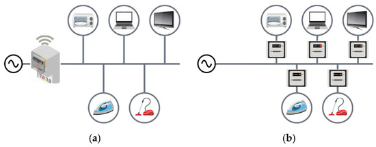
Figure 1.
Schematic of the measurements according to the NILM concept (a) and the ILM concept (b).
The key point of this paper is the use of binary classifiers for multiclass classification and dedicated data selection for this task, which is based on the mRMR method. To improve the reliability of the classification, a further innovation was applied by extending the number of classes of the identified devices. It is also important to highlight the global approach to load identification for the NILM. For this purpose, classes (types) of appliances were identified rather than individual appliances, as is performed in most works. For example, the term ‘hoover’ refers to all vacuum cleaner-type electricity consumers. In this work, each appliance type is represented by several different units, operating in different modes and under different power conditions.
2. NILM—Key Elements
The NILM concept, developed by Hart [1], assumes that the measurement takes place at only one point, as shown in Figure 1a. Thus, the measured signals result from the energy consumption of multiple devices. On the basis of the values obtained in this way, the devices operating in the energy system are identified. From a formal point of view, the task of the NILM system is to identify energy consumers by disaggregating the measured quantities to improve energy efficiency or cost-effectiveness. This is a highly underdetermined task, which means that it cannot be solved by analytical methods [2].
2.1. Milestones
The sensitive stages of the NILM are measurement, data preprocessing, including feature vector selection, model learning, model evaluation, and load identification. Their implementation is interconnected, and the way in which each of them is carried out can influence the results of the other stages. In addition, because the stages listed are very much determined by the analysis scheme adopted, we can analyze the steady state or transient events.
The measurement and associated data acquisition constitute the first stage of the NILM. The frequency at which the measurements are carried out determines the type and range of the parameters that can be extracted from them [3,4,5]. In the case of low-frequency measurements, we must limit ourselves to basic quantities, such as the active power, reactive power, effective current, and power factor. In the case of the data obtained from high-frequency measurements, the harmonics, THD (total harmonic distortion), CF (crest factor), etc., can also be used. In recent years, the popularity of methods that use these types of measurements has increased [4,5,6,7,8]. In practice, low-frequency measurements are mainly used for event analysis.
Feature vector selection aims to select from the collected measurements and their derived magnitudes (computationally determined) those that have the best information properties in the context of device identification. The selection of signatures is often expert-driven and based on experience, but studies using computer-based methods for this purpose are increasingly emerging [7,8,9,10]. A comprehensive overview of the features used for identification can be found in the work of Souza and colleagues [5]. Importantly, feature selection, by eliminating features that do not carry information, results in a reduction in the dimensions of the input data, which benefits the identification process.
The identification of electrical devices for monitoring is carried out via artificial intelligence methods such as artificial neural networks, including deep networks [4,6,7,8,11,12,13,14]; rule-based methods such as decision trees or random forests [15,16,17]; k-nearest neighbors methods (kNN) [4,15,18]; Bayes classifiers and hidden Markov chains [4]; optimization methods [19]; and hybrid methods [20,21,22,23]. In recent years, methods using deep learning networks have become very popular. Their advantage is very good identification results, but the need to use very large data repositories for their learning is a major obstacle. Consequently, most authors base their research on the same data available in public repositories.
2.2. Research Methodology
NILM research is divided according to the many different categories mentioned earlier. It seems worthwhile to further subdivide research into the following:
- Global, covering multiple classes of equipment represented by many different units operating in different states and under different power conditions;
- Local, covering individual devices or treating devices of the same type as other devices.
Many authors use a local approach in their research, treating each piece of equipment as a different device. This approach is easier to implement and yields better results but is practically impossible to generalize because of the wide variety of individual electricity consumers.
Most often, in NILM-related works, the selection of identifying features is expert in nature [5,6,13,14] and mainly includes the active power (P), reactive power (Q), and root mean square (rms) current (I). The harmonics of the active power, reactive power, and current are used less frequently, as their use directly leads to the ‘curse of dimensionality’, the avoidance of which requires the use of analytic feature selection methods.
In [24], Wu and coauthors proposed a multilabel classification method using the random forest method for load identification. Multilabel classification makes it possible to determine the category to which the data belong and allows for the identification of devices in different operating states on the basis of aggregated signals. For the study, the authors used five electrical appliances (two computers of different brands, a printer, a kettle, and a microwave oven) on the basis of data from the laboratory and the BLUED (Building-Level fUlly-labeled dataset for Electricity Disaggregation) database. The way the devices were classified and their number indicate that the proposed research should be localized. To build the model, the authors used basic electrical parameters, such as the rms current, current signal peak factor, maximum current, active power, reactive power, power factor, fundamental harmonic current, and third harmonic current. In the next step, they examined the relevance of each characteristic to the model being built. The rms value of the current and its third harmonic component have the greatest impact on the results, reaching 20%, whereas the reactive power has a small impact of only 1%. The contributions of the rms value of the current and the fundamental harmonic are 16% and 18%, respectively. The contributions of the other parameters are less significant and amount to an active power of 10%, power factor of 9%, and a peak factor of 6%, obtained by the authors, as well as a very high identification accuracy, with an accuracy (6) close to 98%, using expertly selected parameters.
Ciancetta and colleagues [13] presented a method using a convolutional neural network (CNN) for electrical load identification, whose operation is based on the use of deep learning (DP). The CNN used in this study consisted of seven layers. Five appliances were identified—microwave oven, oven, induction hob, toaster, and light—by defining 10 classes (on/off for each) and a no event class. The proposed algorithm corresponded to whether the appliance was on or off. The authors performed tests on data acquired from their own measurement system operating at 10 kHz. Their proposed algorithm showed an error of 1.84% when identifying switch-on events and an error of 1.21% when identifying switch-off events. This means that its accuracy index (6), which describes classification accuracy, was 98%. To compare the results obtained, an experiment was conducted on the BLUED public database. The authors expanded the number of classes to 69 (34 device types), obtaining an accuracy of 87.9%. The number of classes extracted for the BLUED database (not currently available) covering measurements made in a single building indicates that the authors used a local approach.
In [16], the authors used the k-nearest neighbors method to identify appliances for the NILM. The study was carried out with data collected from five homes and uploaded to the public REDD (Reference Energy Disaggregation Data) database. This included the identification of the following seven appliances: cooker, water heater, oven, electronics, waste grinder, washer–dryer, and microwave. To evaluate the performance of the kNN method properly, the dataset was divided into a training part (containing 90% of the data) and a test part (containing 10% of the data). The kNN algorithm identified four appliances without error; only for electronics was the identification at 66.7%. The accuracy coefficient (6) covering the identification accuracy of all devices achieved a value of 92.6%. In this paper, the authors used a global approach and a wide range of potential identification features, which were subjected to analytical selection. The approach presented, concerning the use of a wide set of identification features acquired under a variety of conditions, indicates a potential solution to identification feature selection problems.
In [11], a new approach in which a threshold was used to identify the state of devices on the basis of energy consumption readings was introduced. The feedforward neural-network-based NILM outperformed the traditional logistic regression by 5.78%, whereas the use of the threshold improved the accuracy by an additional 19.1%. The overall performance improvement over logistic regression was 25%.
The authors of [13] proposed a neural NILM algorithm using a convolutional neural network, which simultaneously detects and classifies events while minimizing the computation time. The applied technique transforms current signals into images processed by a CNN, enabling device recognition under various conditions. The results on the BLUED dataset achieved an F1 score of 99.8%, outperforming the other solutions.
In [4], the authors developed a comprehensive NIALM laboratory for testing devices and artificial intelligence methods. The results indicate that the frequency analysis of the EMI (electromagnetic interference) is not feasible with the European power grid. A technique was introduced that utilizes high-frequency signals for device identification, involving the introduction of disturbances to analyze system responses.
In [16], the authors proposed a non-intrusive load monitoring method based on random forest to determine energy consumption by building subsystems. Three feature selection methods were applied and compared to achieve an accurate NILM based on the weather parameters, wavelet analysis, and principal component analysis, ensuring the most accurate results. The method achieved RMS errors below 46.4 kW and relative errors below 12.7%. The NILM allows for the disaggregation of energy consumption signals into individual devices, leading to more conscious energy use and savings. In this study, the K-nearest neighbors algorithm was used for the classification of energy signals. The REDD dataset was used, achieving signal separation for K = 5 after appropriate data processing.
2.3. Representative Data
The artificial intelligence methods used for building the NILM device is modeled on the basis of the data presented to them. Consequently, the quality of the results obtained strongly depends on the representativeness of the data used for learning and testing of the system. In the case of appliance monitoring, to obtain a global model, it is necessary to provide data acquired in different power systems that describe different fashions of the same appliance (hoovers, kettles, etc.).
More than 20 data repositories are well known, mainly from European countries and North America (Table 1). In most cases, data were collected at a low frequency, with only nine databases providing high-frequency data. The authors are most likely to use data from the following databases: REDD and UK-Dale (United Kingdom—Domestic Appliance-Level Electricity), followed by REFIT (Personalised Retrofit Decision Support Tools For UK Homes Using Smart Home Technology), PLAID (Plug-Load Appliance Identification Dataset), WHITED (Worldwide Household and Industry Transient Energy Data), and LILAC (Learnable Image-Based Load Signature Construction Approach) [25] (Figure 2). The authors of [25] sometimes used the energy demand model to generate training data and, thus, eliminated the need for historical measurement data.

Table 1.
List of data repositories used in NILM studies.
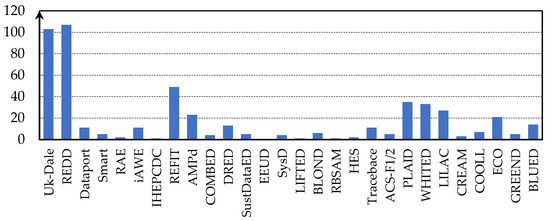
Figure 2.
Occurrence of data repositories in articles. Reprinted with permission from Ref. [25]. Copyright 2023, Norbert Solarz.
3. Electricity Consumers and Potential Identification Characteristics
The research presented in this article involves the identification of 12 types of single-phase, two-state, and multistate electrical devices with a finite number of states and an infinite number of operating states (Table 2).
Table 2.
List of electricity consumers covered by the tests.
The features used to describe the devices were obtained from measurements made with an Elspec BlackBox G4500 power quality analyzer. The Elspec is a device that is equipped with 11 measurement channels, which allows for the simultaneous measurement of voltages and currents in each phase. In each period, the voltage is sampled 1024 times and the current 256 times. Dedicated PQScada version 4.2 software allows for the transfer of measurement data from the analyzer to a database with an MS SQL engine. Full analysis of the data collected in the system can be performed using the dedicated PQInvestigator version 4.2 software. The application allows for the visualization and processing of the collected data, as well as their export in popular formats. Measurement data were collected from 11 sites (buildings) supplied by various transformer stations. Each class of equipment was represented by 4–5 different units; for each unit, many forced steady-state measurements were performed. The resulting data set was balanced.
The measurement frequency was 51.2 kHz, making it possible to use a very wide range of potential identification features, including the following:
- The rms values of the voltage:
- Total U;
- Higher harmonics Uh;
- 50-First harmonics U1 ÷ U50.
- Rms values of the current:
- Total I;
- Higher harmonics Ih;
- 50-first harmonics I1 ÷ I50.
- Active capacities:
- Total P;
- Higher harmonics Ph;
- 50-First harmonics P1 ÷ P50.
- Passive powers according to Budeanu:
- Total Q;
- Higher harmonics Qh;
- 50-First harmonics Q1 ÷ Q50.
- Apparent powers:
- Total S;
- Higher harmonics Sh;
- Of the primary component S1.
- Power factors:
- Total PF;
- Higher harmonics Ph;
- Of the primary component P1.
- Harmonic content ratios:
- In voltage THDu;
- In the current THDI.
- Peak factors:
- Voltages CFu;
- Current CFI.
The selection of the harmonic spectrum used in the study considered the recommendations of EN 50160 [26] and IEC 61000-4-30 (EN-61000-4-30) [27], which present the measurement methodology and define the requirements for instruments used for power quality testing, including current and voltage distortion.
4. Feature Selection—mRMR Method
Feature selection is a very important stage of the NILM. Its aim is to select, from the available set of features, those that carry as much information about the receiver as possible. In the case of a large set of potential identification features, feature selection also leads to a reduction in the dimensions of the input data. For the purposes of this study, the mRMR selection method was used.
The mRMR method is based on issues in information theory and the correlations between features describing an element (in our case, an electricity receiver). The algorithm aims to select the most relevant features that are, at the same time, as least dependent among themselves, so it selects features with a high correlation with the class (in our case, the receiver understood as an entity) and low correlation among themselves.
The significance, D, of the feature set, S, for class c is determined by the average value of all mutual information values, G, between individual feature, f, and class, c, as follows:
The redundancy, R, of all features in the set, S, is determined as the mean value of all mutual information values between the features fi and fj, as follows:
Using the measures of significance and redundancy defined above, the relevance, M, of each feature to the class description is determined as follows:
The features are selected one at a time via a greedy algorithm to maximize the objective function, which is a function of the relevance and redundancy.
The selection of features of the electrical appliances via the mRMR method was carried out on the entire learning set, maintaining an independent description of each appliance. As a result of this study, we obtained significant values for individual parameters, as shown in Figure 3. An analysis of the figure allows us to conclude that most of the features are, according to the mRMR method, completely insignificant, as their significance coefficient values are close to 0.
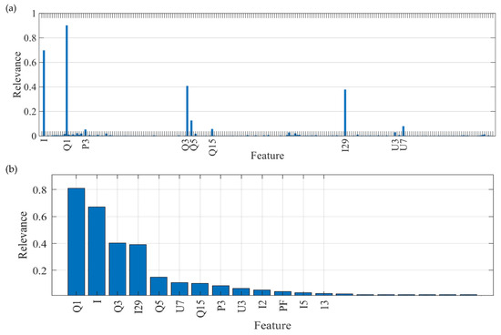
Figure 3.
Significance coefficient values of identification features determined via the mRMR method: (a) all features in order of occurrence; (b) features in order of significance.
It was decided that the following features would be used to learn and test a classifier for identifying electrical equipment:
- Reactive power of the first harmonic, Q1;
- Rms value of current, I;
- Reactive power of the third harmonic, Q3;
- Rms value of the twenty-ninth harmonic current, I29;
- Reactive power of the fifth harmonic, Q5.
5. Classifiers Used for Identification
Two classifiers using artificial intelligence were developed for identification purposes, as follows: one based on artificial neural networks and the other on decision trees. Data processing in both classifiers is a two-stage process. First, the data are sent to the preclassification module, which identifies potential workloads. The answers provided are then evaluated by the decision module, which provides the final answer.
5.1. Neural Classifier with a Decision Module
The preclassification module of the neural classifier consisted of a set of neural networks (Figure 4), each of which was used to classify a device into one class—providing an answer to the following: Does the identification vector describe the device? The networks have an identical structure and consist of 5 neurons in the input layer, 15 in the hidden layer, and 1 in the output neuron. The number of neurons in the input layer is dictated by the length of the input vector, whereas the number of neurons in the input layer is the number of distinguishable classes. Owing to the lack of analytical methods for determining the number of hidden layer neurons [28], this selection was made experimentally (networks with 1 hidden layer and 2 hidden layers were tested). Similarly, a tangential transition function was selected for these layers, while the output layer neurons were fitted with a linear transition function. The Levenberg–Marquardt method, characterized by high efficiency and speed of learning, was used to teach the network [29].
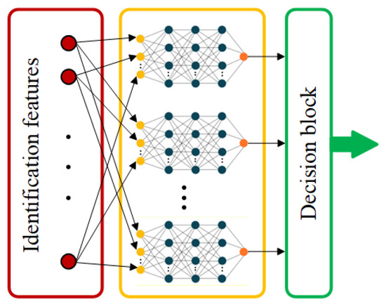
Figure 4.
Schematic of a classifier based on artificial neural networks.
The decision block determines the final response of the system according to the following principle: if only one of the networks has indicated a device, then this device is recognized, and this response is given at the output of the system. If more than one network indicates that ‘its’ device is working, the decision module compares the response values and points to the one that has been most strongly indicated (the network response value is the highest), which can be described by the following relation:
where
- Decision—decision of the classifier;
- Yi—the response of the i-th neural network.
5.2. Decision Trees with a Decision-Making Module
The classifier using decision trees had a structure analogous to that of the neural classifier; it consisted of two modules. The first is a set of decision trees, each adapted to recognize a single device. The second is the deciding module, which provides the final answer according to the following rules:
- If only one tree has identified a device, its response is that of the following classifier:
- If no tree has given a positive answer, the classifier answers ‘do not know’, as follows:
- If several trees have given a positive answer, the classifier also answers ‘do not know’, as follows:
The CART (classification and regression trees) algorithm, which uses a binary division of the input elements for its operation, was used to construct decision trees. At each node of the tree, the dataset is divided into two subsets, and the division of the data is implemented via the Gini criterion, which divides the input set into possibly homogeneous result sets. The remaining tree parameters were chosen experimentally.
6. Test Results
6.1. Indicators for Assessing the Quality of Identification
Four indicators were selected to assess the quality of identification, as follows: Accuracy, Precision, Recall, and F1.
The Accuracy metric indicates what proportion of the data were classified correctly. It indicates the probability of correctly identifying an average device.
where
- TP—the number of elements belonging to the class and correctly classified into it;
- FP—number of elements not belonging to the class and misclassified in the class;
- FN—number of elements belonging to the class and not classified in the class;
- TN—number of elements not belonging to a class and not classified in a class.
The Precision indicator indicates the extent to which we can trust positive identifications. It indicates the probability that, if the system identifies a device, a signal from that device has actually been given to its input, as follows:
Recall is an indicator of the probability with which a class will be correctly recognized. This indicates the probability that if a signal from a specific device is applied to the system input, it will be correctly recognized as follows:
The F1 measure is the harmonic mean of the Precision and Recall indicators. The choice of the harmonic mean instead of the arithmetic mean makes this indicator more sensitive to results close to zero. Owing to this property, it is easy to see if one of the indicators (Precision or Recall) has a very small value.
The selected indicators are the most readily used indicators to assess the quality of identification, as they capture the features relevant to classification.
Using the data selected by the mRMR method and the classifiers described in Section 4, the identification of the electricity consumers listed in Section 3 was carried out. Performance tests of the defined classifiers were performed. The Repeated Holdout method [30] was used to obtain a correct estimation of the quantities used to assess the quality of the identification. A total of 1000 learning and testing operations were performed, each time dividing the dataset into two subsets Figure 5, as follows: learning subset (90%) and test subset (10%).
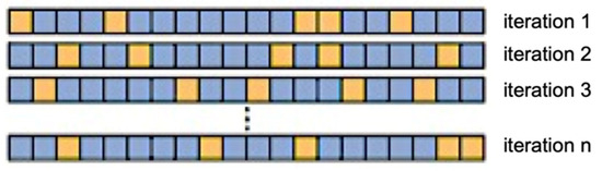
Figure 5.
Schematic for selecting the partitioning of the dataset into teaching and testing sets in the Repeated Holdout method.
6.2. Neural Classifier Supported by a Decision-Making Module
Using a neural classifier, an average identification accuracy expressed by an Accuracy index of 88.8% was obtained. Table 3 summarizes the values of the evaluation coefficients analyzed. The first column shows the names of the devices whose features describing their operation were given to the input of the classifier, whereas the first row shows the names of the devices that were identified on the basis of these features. Thus, the values on the diagonal represent the number of appliances identified correctly by Recall as a percentage, whereas the other values in the row represent the number of appliances identified incorrectly with the class into which they were classified (in the case of a value of 0, the cell is left blank). The best identified appliances were toasters (95.9 per cent), whereas the most trusted identifications were hoovering (98.8 per cent) and grinders (98.3 per cent). The greatest problems occurred with the identification of blenders, with a Recall of 77.3% and Precision of 73.9%.
Table 3.
Recall, Precision, and F1 [%] values for the identification of energy consumers with a classifier via artificial neural networks.
6.3. Decision Trees with a Decision-Making Module
For the classifier based on decision trees, the average identification Accuracy was 89.1%. Table 4 shows the values of the coefficients for assessing the identification quality. The best identification quality and response reliability were obtained for hoovers (Recall of 93.7% and Precision of 98.3%). Microwaves were also identified very well (Recall of 98.1%).
Table 4.
Recall, Precision, and F1 [%] values for the identification of energy consumers with a classifier via decision trees.
6.4. Comparison of Classifiers
The identification accuracies of the two classifiers tested, as measured by the Accuracy index, were very similar at approximately 89% (neural classifier: 88.8%; decision trees: 89.1%).
The introduction of an additional ‘do not know’ class for the decision-tree-based classifier resulted in an increase in the value of the Precision coefficient—for all devices, its value exceeds 90% (Table 5)—and there was an equalization of its value for individual electricity consumers. Consequently, the reliability of the answers returned by the decision-tree-based classifier is significantly greater (average Precision: 96.8%, which should be considered a very good result) than the reliability of the answers of the neural classifier (88.8%) (Figure 6).
Table 5.
Summary of the extreme and average Recall, Precision, and F1 [%] values for both classifiers.
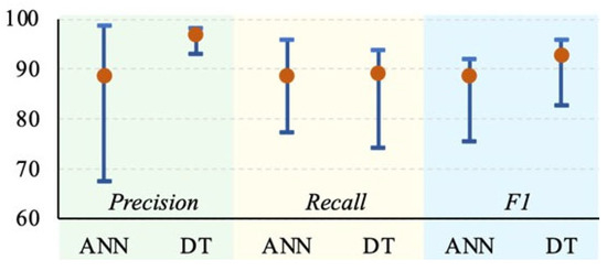
Figure 6.
Visualization of the extreme and average Precision, Recall, and F1 values [in %] for both classifiers.
The values of the Recall indices for both classifiers are similar (Table 5 and Figure 6). The minimum and maximum values of this index are greater for the classifier using neural networks, but the average value is greater for the classifier built on decision trees.
The F1 index, which is the harmonic mean of the Precision and Recall, indicates a slight advantage for the classifier using decision trees; both the extreme values and the mean for this classifier have higher values than those for the classifier built via artificial neural networks.
7. Conclusions
This paper proposes a novel approach to identifying electricity consumers for the NILM. It is based on the use of binary identification to implement multiclass classification. The results show that this approach achieves high-quality identification of electricity consumers.
The study included 12 devices. Identification features were selected via analytical methods from a set of practically all possible features. The optimization criterion for feature selection was minimal redundancy between features and maximal correlation of a feature with a decision class. The presented research analyzes and identifies single electrical devices, with a non-additive description of the identification features returned by the analyzer. Transforming the features to an additive form, requiring phase-angle measurement, will solve this problem.
It has been shown that it is possible to improve the reliability of the classifier’s response by introducing an additional class (‘do not know’) into which items are placed when the response of the binary identification module is ambiguous. In further research, the possibility of designing an identification module that correctly identifies the elements included in the ‘do not know’ class while maintaining the level of response reliability should be investigated.
An Elspec BlackBox G4500 Class A analyzer was used to collect the large amount of data required for the training processes. The results show that of the set of features listed in the work, only five, according to the mRMR criterion, have valuable identification properties, and only these need to be extracted during system operation. At this stage of the research, one relevant features is the higher harmonic current, the measurement of which requires a meter with a high sampling rate. Currently, there are inexpensive measurement systems whose use solves this problem.
The use of high-frequency measurements made it possible to compile a very broad set of 218 potential identification features. From this set, via the mRMR method, a set of features describing the receivers was selected. The resulting data set has an analytically determined composition defined by the devices under study and contains non-obvious identifying features. The selection of features is mostly exploratory in nature, and the presented research indicates that the use of analytical methods for this purpose can point to previously unused features as valuable sources characterizing the operation of devices.
The research presented here is global in nature, and care was taken during implementation to ensure that each class of the equipment was represented by several different units operating in different operating states and under different power conditions.
Author Contributions
J.B. conceived the methodology of the research, measurement data, and software and wrote all of the manuscript text; B.K. was responsible for data preprocessing; D.M. interpreted the experimental results from the power and electrical engineering perspectives; P.K. prepared the drawings and charts; B.T. tested the models and reviewed related works. All authors have read and agreed to the published version of the manuscript.
Funding
This research received no external funding.
Institutional Review Board Statement
Study did not require ethical approval.
Informed Consent Statement
Not applicable.
Data Availability Statement
Conflicts of Interest
The authors declare no conflicts of interest.
References
- Hart, G.W. Nonintrusive Appliance Load Monitoring. Proc. IEEE 1992, 80, 1870–1891. [Google Scholar] [CrossRef]
- Schirmer, P.A.; Mporas, I.; Sheikh-Akbari, A. Robust energy disaggregation using appliance-specific temporal contextual information. EURASIP J. Adv. Signal Process. 2020, 3, 1–13. [Google Scholar] [CrossRef]
- Schirmer, P.A.; Mporas, I. Non-Intrusive Load Monitoring: A Review. IEEE Trans. Smart Grid 2023, 14, 769–784. [Google Scholar] [CrossRef]
- Wójcik, A.; Łukaszewski, R.; Kowalik, R.; Winiecki, W. Nonintrusive Appliance Load Monitoring: An Overview, Laboratory Test Results and Research Directions. Sensors 2019, 19, 3621. [Google Scholar] [CrossRef]
- Souza, W.A.; Alonso, A.M.S.; Bosco, T.B.; Garcia, F.D.; Gonçalves, F.A.S.; Marafão, F.P. Selection of features from power theories to compose NILM datasets. Adv. Eng. Inform. 2022, 52, 101556. [Google Scholar] [CrossRef]
- Tokam, L.W.; Ouro-Djobo, S.S. Comparative Study on Load Monitoring Approaches. Appl. Sci. 2023, 13, 5755. [Google Scholar] [CrossRef]
- Bartman, J.; Kwater, T. Identification of Electrical Appliances Using Their Virtual Description and Data Selection for Non-Intrusive Load Monitoring. IEEE Trans. Consum. Electron. 2021, 67, 393–401. [Google Scholar] [CrossRef]
- Bartman, J. Analiza zborności parametrów odbiorników energii elektrycznej w kontekście bezinwazyjnej identyfikacji urządzeń. Przegląd Elektrotechniczny 2022, 1, 267–270. [Google Scholar] [CrossRef]
- Bao, S.; Zhang, L.; Han, X.; Li, W.; Sun, D.; Ren, Y.; Liu, N.; Yang, M.; Zhang, B. Feature Selection Method for Nonintrusive Load Monitoring with Balanced Redundancy and Relevancy. IEEE Trans. Ind. Appl. 2022, 58, 163–172. [Google Scholar] [CrossRef]
- Huang, J.; Xue, Y.; Liu, L. Dynamic Signature Verification Technique for the Online and Offline Representation of Electronic Signatures in Biometric Systems. Processes 2023, 11, 190. [Google Scholar] [CrossRef]
- Fazzil, N. Non-intrusive load monitoring for appliance status determination using feed-forward neural network. Przegląd Elektrotechniczny 2022, 1, 29–34. [Google Scholar] [CrossRef]
- Lin, L.; Liu, J.; Huang, N.; Li, S.; Zhang, Y. Multiscale spatiotemporal feature fusion based non-intrusive appliance load monitoring for multiple industrial. Appl. Soft Comp. 2024, 167, 112445. [Google Scholar] [CrossRef]
- Ciancetta, F.; Bucci, G.; Fiorucci, E.; Mari, S.; Fioravanti, A. A New Convolutional Neural Network-Based System for NILM Applications. IEEE Trans. Instrum. Meas. 2021, 70, 1–12. [Google Scholar] [CrossRef]
- Cannas, B.; Carcangiu, S.; Carta, D.; Fanni, A.; Muscas, C. Selection of Features Based on Electric Power Quantities for Non-Intrusive Load Monitoring. Appl. Sci. 2021, 11, 533. [Google Scholar] [CrossRef]
- Lemes, D.A.M.; Cabral, T.W.; Fraidenraich, G.; Meloni, L.G.P.; De Lima, E.R.; Neto, F.B. Load Disaggregation Based on Time Window for HEMS Application. IEEE Access 2021, 9, 70746–70757. [Google Scholar] [CrossRef]
- Ling, Z.; Tao, Q.; Zheng, J.; Xiong, P.; Liu, M.; Xiao, Z.; Gang, W. A Nonintrusive Load Monitoring Method for Office Buildings Based on Random Forest. Buildings 2021, 11, 449. [Google Scholar] [CrossRef]
- Solorio-Ramírez, J.-L.; Jiménez-Cruz, R.; Villuendas-Rey, Y.; Yáñez-Márquez, C. Random forest Algorithm for the Classification of Spectral Data of Astronomical Objects. Algorithms 2023, 16, 293. [Google Scholar] [CrossRef]
- Ozturk Kiyak, E.; Ghasemkhani, B.; Birant, D. High-Level K-Nearest Neighbors (HLKNN): A Supervised Machine Learning Model for Classification Analysis. Electronics 2023, 12, 3828. [Google Scholar] [CrossRef]
- Gao, Z. Special Issue on “Modelling, Monitoring, Control and Optimization for Complex Industrial Processes”. Processes 2023, 11, 207. [Google Scholar] [CrossRef]
- Andrean, V.; Zhao, X.-H.; Teshome, D.F.; Huang, T.-D.; Lian, K.-L. A Hybrid Method of Cascade-Filtering and Committee Decision Mechanism for Non-Intrusive Load Monitoring. IEEE Access 2018, 6, 41212–41223. [Google Scholar] [CrossRef]
- Lu, M.; Li, Z. A Hybrid Event Detection Approach for Non-Intrusive Load Monitoring. IEEE Trans. Smart Grid 2019, 11, 528–540. [Google Scholar] [CrossRef]
- Fang, Z.; Zhao, D.; Chen, C.; Li, Y.; Tian, Y. Non-Intrusive Appliance Identification with Appliance-Specific Networks. IEEE Trans. Ind. Appl. 2020, 56, 3443–3452. [Google Scholar] [CrossRef]
- Abbas, M.Z.; Sajjad, I.A.; Hussain, B.; Liaqat, R.; Rasool, A.; Padmanaban, S.; Khan, B. An adaptive-neuro fuzzy inference system based-hybrid technique for performing load disaggregation for residential customers. Sci. Rep. 2022, 12, 2384. [Google Scholar] [CrossRef]
- Wu, X.; Gao, Y.; Jiao, D. Multi-Label Classification Based on Random Forest Algorithm for Non-Intrusive Load Monitoring System. Processes 2019, 7, 337. [Google Scholar] [CrossRef]
- Solarz, N. Analysis of Data Repositories Used in Non-Invasive Load Monitoring. Rzeszów, 2023. Available online: https://wu.ur.edu.pl/PromotorPraceDyplomantow.aspx (accessed on 30 June 2023).
- EN 50160; Voltage Characteristics of Electricity Supplied by Public Distribution Systems. PKN: Warsaw, Poland, 2023.
- IEC 61000-4-30; Electromagnetic Compatibility. Testing and Measurement Techniques–Current Quality Measurement Methods. PKN: Warsaw, Poland, 2021.
- Gomolka, Z.; Twarog, B.; Zeslawska, E.; Lewicki, A.; Kwater, T. Using Artificial Neural Networks to Solve the Problem Represented by BOD and DO Indicators. Water 2017, 10, 4. [Google Scholar] [CrossRef]
- Cai, Y.; Jelovica, J. Neural network-enabled discovery of mapping between variables and constraints for autonomous repair-based constraint handling in multi-objective structural optimization. Knowl. Based Syst. 2023, 280, 111032. [Google Scholar] [CrossRef]
- Allgaier, J.; Pryss, R. Cross-Validation Visualized: A Narrative Guide to Advanced Methods. Mach. Learn. Knowl. Extr. 2024, 6, 1378–1388. [Google Scholar] [CrossRef]
Disclaimer/Publisher’s Note: The statements, opinions and data contained in all publications are solely those of the individual author(s) and contributor(s) and not of MDPI and/or the editor(s). MDPI and/or the editor(s) disclaim responsibility for any injury to people or property resulting from any ideas, methods, instructions or products referred to in the content. |
© 2025 by the authors. Licensee MDPI, Basel, Switzerland. This article is an open access article distributed under the terms and conditions of the Creative Commons Attribution (CC BY) license (https://creativecommons.org/licenses/by/4.0/).