Localization of Conveyor Belt Damages Using a Deep Neural Network and a Hybrid Method for 1D Sequential Data Augmentation

Abstract

The article describes an innovative method for detecting conveyor belt damage using a strain gauge system and deep learning techniques. The strain gauge system records measurement data from conveyor belts. A major challenge encountered during the research was the insufficient amount of measurement data for effectively training deep neural networks. To address this issue, the authors implemented a hybrid data augmentation method that combines generative artificial intelligence techniques and signal analysis. The TimeGAN model, based on Generative Adversarial Networks (GANs), was used to augment data from undamaged belts. Meanwhile, the superposition of one-dimensional observation sequences was applied to generate data representing damages by combining signals from randomly selected undamaged runs with strain gauge system responses to damage, effectively increasing the number of samples while accurately replicating defect conditions. For damage diagnosis, a Long Short-Term Memory Network with an attention mechanism (LSTM-AM) was employed, enabling anomaly detection in strain gauge signals. The application of the LSTM-AM algorithm allows for real-time monitoring of conveyor operation and facilitates precise localization and estimation of damage size through data synchronization.

1. Introduction

Conveyor belts play a crucial role in material transportation systems due to their ability to operate continuously and reliably. They are widely used in various industries, such as mining, logistics, and manufacturing, thanks to their versatility, flexibility, and efficiency. Conveyor belts can transport large quantities of different materials under various working conditions over long distances in a continuous manner, significantly improving process efficiency. Additionally, they offer lower operational costs and greater environmental benefits compared to other transportation methods, such as road or rail transport. Over the years, extensive laboratory research has led to the development of advanced solutions for conveyor belt construction, operation, applications, monitoring, and control methods [1,2].

Conveyor belts can be used in production halls, mines, and open spaces, serving both single devices and extensive transportation systems. The diagnostics of conveyor belts primarily involves inspecting the belt itself as a material carrier, along with drive components, motors, gear mechanisms, and other structural elements. Conveyor belts are one of the most challenging components to diagnose, particularly in cases of damage caused by physical, chemical, or biological factors. Typical belt damages include mechanical issues such as cuts, punctures, and dents, as well as chemical, thermal, or biological deterioration. Early detection of such issues enables preventive measures, thereby extending the lifespan of conveyors [3,4].

Diagnostic methods encompass a wide range of non-destructive testing techniques using Industry 4.0 technologies. Real-time monitoring, supported by artificial intelligence tools and deep learning models, has a direct impact on the efficiency and safety of conveyor belt operations [5,6]. Ultrasonic sensors and vibroacoustic analysis help detect cracks and other conveyor belt damages, as well as issues with bearings, drums, and other drive components [7,8,9]. Vision and thermographic systems utilize cameras and image analysis algorithms to monitor the belt’s condition, identifying visible surface damage such as cracks and abrasions while also detecting drive-related issues [10,11,12,13].

The literature studies indicate that the development of conveyor belt monitoring systems is dynamic. The projected increase in expenditures on such technologies highlights their growing importance in optimizing production processes. The integration of non-destructive testing methods with machine learning algorithms and advanced data acquisition techniques contributes to improved reliability and reduced operational costs of conveyor systems. However, measurement data collected under industrial conditions are often affected by various factors that negatively impact data quality [14].

Existing solutions for detecting and identifying damage in conveyor belts, while effective in many applications, often face specific challenges. These include the precise localization of damage in fabric-based belts and the frequent requirement for expensive and specialized equipment, such as belts with embedded sensors, probes, or additional diagnostic devices. Furthermore, many of these methods necessitate planned conveyor shutdowns for inspection, leading to potential downtime. Their effectiveness can also be limited to detecting specific damage types, depending on their orientation and the diagnostic technology employed. In this context, the strain gauge system presents an attractive complementary or alternative solution, distinguished by its low implementation and operational costs. Its key advantage lies in its ability to continuously measure loads and stresses in real time, without the need for structural intervention in the belt or stopping the conveyor.

This enables the early detection of subtle changes in the transport system’s operation, which can indicate potential issues such as belt deformation, pulley misalignment, or uneven wear. While the strain gauge system does not directly measure belt thickness or offer the same precise tear localization as more advanced methods like ultrasonic or laser systems, it serves as an effective and cost-efficient early warning tool. It is an ideal choice when low cost and simple integration are priorities. However, when precise tear detection and wear prediction are critical, advanced systems remain the optimal choice. The research presented in this paper aims to develop and test a monitoring system that, through a unique combination of early warning capabilities and cost effectiveness, minimizes or eliminates the aforementioned limitations, offering a valuable solution for a wide range of applications.

In real-world industrial conditions, the number of defective components is relatively low compared to properly functioning elements. Consequently, there is a limited number of labeled fault samples, which poses a challenge for optimizing generative deep learning models and feature extraction methods. These methods aim to reduce subjectivity in user-driven selection tasks and enhance training datasets [15,16,17,18].

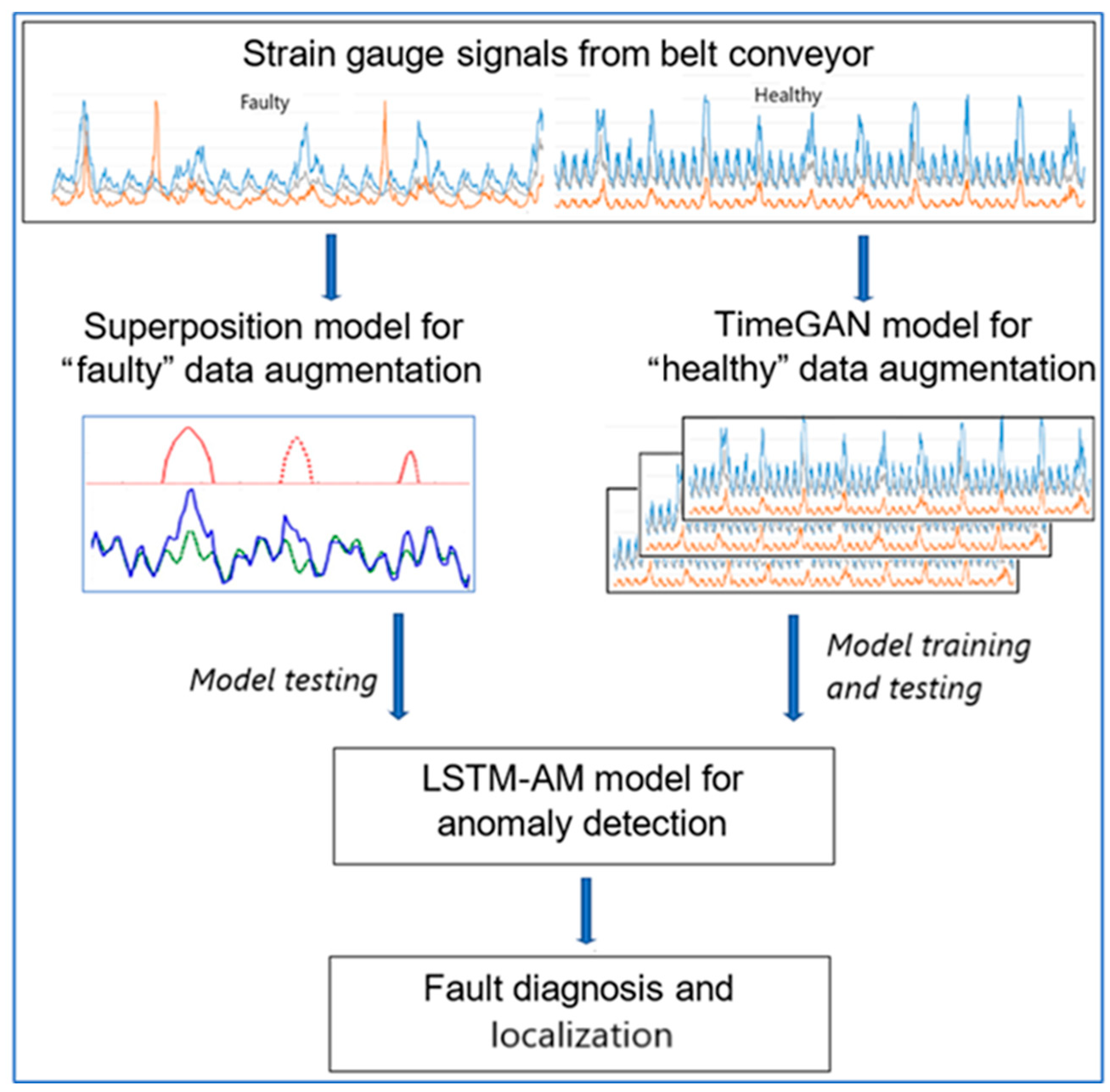
In the proposed solution, measurements were conducted using a specially designed strain gauge system mounted on one of the conveyor model’s rollers [5,19]. The current research focuses on methods for generating synthetic data to simulate various operational scenarios or rare conveyor belt conditions. Due to the insufficient amount of training data for deep neural networks, a hybrid data augmentation method was implemented. For generating sequences of undamaged data, a TimeGAN model—a Generative Adversarial Network (GAN) designed for time series data—was used. Meanwhile, to create sequences representing damages, a signal mixing strategy was applied, combining randomly selected undamaged signals with strain gauge responses to belt damage. Damage detection was performed using an LSTM-AM (Long Short-Term Memory–Attention Model) algorithm, which identifies anomalies in strain gauge signals. Through data synchronization, the system was able to determine the exact location of the damage.

The reasoning method is schematically presented in Figure 1.

The novelty of the proposed solution lies in integrating advanced sequential data augmentation methods with modern deep learning algorithms for conveyor belt diagnostics. The hybrid data generation approach, combining TimeGAN with superposition of one-dimensional observation sequences, represents a breakthrough in addressing the challenge of limited sample availability in diagnostic research. Furthermore, applying the LSTM-AM algorithm to strain gauge signal analysis not only enables damage detection but also allows precise localization, which is crucial for improving conveyor belt safety and efficiency.

The article is structured as follows: Section 1 presents the main problem and a literature review on conveyor belt damage detection methods. Section 2 discusses the deep learning algorithms used for data augmentation using signal superposition and anomaly detection. Section 2.4 describes the methodology for data collection in the experimental setup. Section 3 applies the described AI algorithms to the research objectives and discusses the results. Section 4 provides a summary and conclusions.

2. Materials and Methods

2.1. Data Augmentation

2.1.1. Data Augmentation Methods

In machine diagnostics, imbalanced datasets are common, as failures occur less frequently than normal operations. Collecting failure data is challenging, costly, and time consuming, while failures themselves can be unpredictable and diverse. Historical data are often incomplete or lack detailed failure records, particularly in older monitoring systems. As a result, datasets are dominated by normal operations, making it difficult for machine learning algorithms to effectively process the minority class representing failures.

This imbalance can lead to biased models that favor the majority class, resulting in poor fault detection performance. Balanced datasets are crucial in deep learning because they enable models to learn and generalize effectively for all classes, avoiding artificially high accuracy caused by predicting only the majority class. Balanced data better reflect actual model performance, minimizing overfitting risks and increasing the model’s robustness to distribution variability. To address the issue of imbalance, techniques such as data augmentation, class weighting, and synthetic oversampling are used. These approaches enable fairer and more reliable training of deep learning models, improving their applicability in real-world scenarios.

In this study, database augmentation was approached in a hybrid manner. Additional samples for fault-free cases were generated using the TimeGAN network, while for faulty cases, a superposition was applied, combining a fault-free signal with the system response to damage-induced excitation.

The authors employed two distinct augmentation strategies to effectively increase and balance the strain gauge measurement dataset. For generating synthetic data representing an undamaged state, the TimeGAN (Time-Series Generative Adversarial Network) model was utilized. TimeGAN is an advanced generative model, a variant of GANs specifically adapted for time series. It combines GAN and autoencoder features, using hybrid training (both supervised and unsupervised) to effectively learn and replicate complex temporal dependencies and properties of the original data. This is crucial for precisely modeling “normal” system behavior, which serves as a reference point for anomaly detection.

For rare fault data, a superposition method of one-dimensional observation sequences was applied. This procedure involves inserting segments of signals characterized by defects (simulated system responses to local damages) into randomly selected locations within a healthy signal. The amplitude of the damage signal is scaled to match actual defect conditions. This pragmatic and effective approach to augmenting rare, critical events ensures the physical plausibility of the generated defects. This method, based on explicit domain knowledge, directly addresses the problem of extreme data scarcity for faults, avoiding challenges such as “mode collapse” often encountered in generative models trained on very limited examples.

Compared to other 1D data augmentation methods, the approach in the article stands out significantly. Simpler transformation-based methods, such as jittering, scaling, permutation, slicing, or time warping, while computationally inexpensive, often fail to preserve complex temporal dependencies or generate truly novel, realistic patterns, which is crucial for sensor data. TimeGAN and superposition offer significantly higher fidelity and domain relevance. Although other generative models exist, such as Variational Autoencoders (VAEs), other GAN variants (e.g., Conditional GANs, Wasserstein GANs, SeriesGAN), and emerging Diffusion Models, their application to extremely rare and critical fault data still faces challenges related to learning from very few examples, such as training instability or “mode collapse.”

The innovativeness of the methods applied in the article lies in the strategic distinction and application of two fundamentally different augmentation methods for distinct data classes. This hybrid approach effectively solves the problem of imbalanced datasets, increasing both the pool of healthy data and systematically expanding the minority class (faults).

2.1.2. Augmentation of Healthy Data Using TimeGAN

TimeGAN (Time-Series Generative Adversarial Network) is a model designed for generating synthetic time series, utilizing both unsupervised and supervised training [20,21,22,23]. TimeGAN consists of four core components (Figure 2):

• Embedder: Transforms time series data into lower-dimensional representations using recurrent neural networks (RNNs) to capture temporal dependencies.
• Recovery: Converts lower-dimensional representations back into synthetic time series data, enabling reconstruction of input data from their representations.
• Generator: Produces representations of time series data based on random noise as input. It uses recurrent neural networks (RNNs) to learn temporal dependencies in the data.
• Discriminator: Evaluates whether data originate from real sources or were generated by the generator.

Through this process, TimeGAN is capable of generating synthetic time series that maintain the temporal structures and properties of the original data [24]. Both supervised and unsupervised learning play essential roles in generating synthetic time series data. The Embedder and Recovery modules are trained in a supervised manner, where the loss function measures the difference between real data and the data reconstructed by Recovery, optimizing the model. The Generator and Discriminator are trained in an unsupervised manner, typical of GAN architectures, where the generator attempts to deceive the discriminator while the discriminator learns to distinguish between real and synthetic data. During sampling, the generator outputs data to the embedding space, and the Recovery model generates synthetic time series data.

2.1.3. Augmentation of Faulty Samples Using the Superposition of 1D Observation Sequences

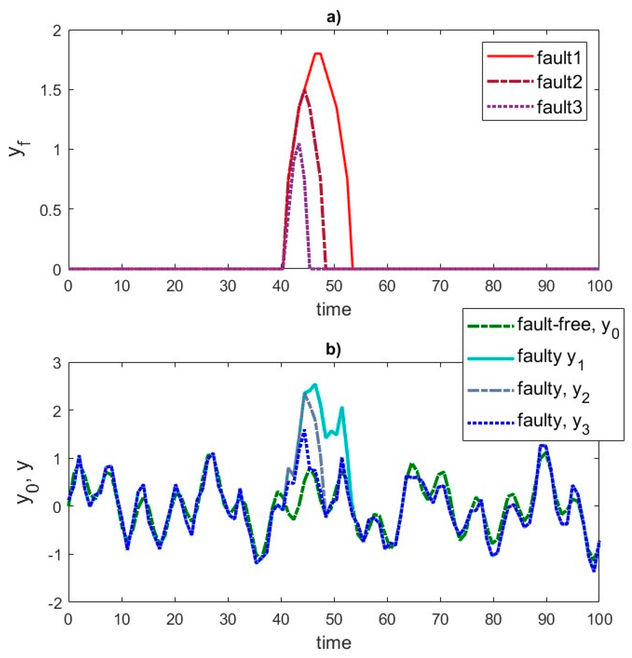
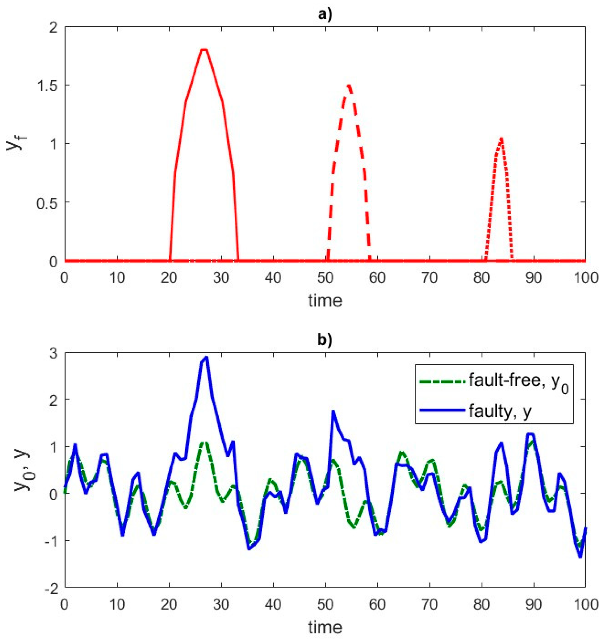
To artificially generate data representing system responses to various excitations, including faults, a superposition of one-dimensional observation sequences can be applied. This procedure involves defining the system response to different types of faults and generating the system response to the given excitations.

In this case, the system responses to local damages, $y_f(t-\tau )$, where $\tau$ indicates the moments of damage occurrence, were simulated, knowing the recorded system responses in the undamaged state, $y_0\left(t\right)$, and in the damaged state, $y\left(t\right)$.

To determine the system response in the damaged state, given the system response in the undamaged state and the system response to local damage, the signal was divided into time segments and segments corresponding to typical tape damage patterns were identified. Then, fragments characterized by defects were inserted in randomly selected locations. Additionally, the amplitude of the damage signal was scaled to match the actual conditions of defect occurrence

$$y\left(t\right)=k_0{y}_0\left(t\right)+\sum _i{k}_i{y}_f\left(t-{\tau }_i\right)$$

(1)

The first component of the equation is the system response in the undamaged state, and the second represents the impact of locally scaled damages (shifted by ${\tau }_i$) on the system response.

The method of generating synthetic responses recorded by the strain gauge is shown in illustrative Figure 3 and Figure 4.

2.2. Implementation of the LSTM-AM Network for Anomaly Detection in Time Series

Anomaly detection in one-dimensional time series signals is a critical task across various domains, from machine diagnostics to health monitoring, as it enables the identification of unusual patterns that may signal failures, errors, or other critical events. Given the sequential nature and temporal dependencies inherent in 1D signals, such as those from strain gauges, specialized analytical methods are essential.

Anomaly detection models broadly fall into statistical, traditional machine learning, and deep learning categories. Statistical methods compare current data points against a statistical model of normal behavior. While simple to implement, they often struggle with complex, high-dimensional, or noisy data, and are less adept at detecting subtle or non-linear anomalies. Traditional machine learning approaches, such as Isolation Forest, One-Class SVM (OCSVM), and K-Nearest Neighbors (KNN), learn normal data behavior to identify significant deviations. These can be effective for lower-dimensional data and may handle some class imbalance, but their performance can be hampered by noise or irrelevant features, and they often require manual feature engineering.

Deep learning methods, with their multi-layered architectures, excel at processing high-dimensional and unstructured data, automatically learning complex patterns and temporal dependencies. Autoencoders (AE/VAE) are trained on normal data to reconstruct it, with high reconstruction error indicating an anomaly. Generative Adversarial Networks (GANs) can model normal data distributions, detecting anomalies when a discriminator easily distinguishes a sample as fake; however, they face challenges like training instability and “mode collapse”. Diffusion Models, a newer generative approach, learn normal data distributions through iterative denoising, offering high stability and complex distribution modeling, though inference speed can be a concern. Recurrent Neural Networks (RNNs) and Long Short-Term Memories (LSTMs) are inherently suited for sequential data, capturing long-term temporal dependencies, and identifying anomalies as deviations from learned normal patterns.

Long Short-Term Memory (LSTM) networks are well suited for analyzing sequential data, such as time series, as they can capture long-term dependencies. Anomaly detection using LSTM relies on modeling normal signal behavior. Once trained on non-anomalous data, the network can identify deviations from typical patterns [25]. LSTM networks incorporate specialized memory cells capable of storing information over long periods, making them more effective in capturing long-term dependencies compared to traditional RNNs. Due to their architecture, LSTM networks are also less susceptible to the vanishing gradient problem, which often occurs in neural networks trained on long sequences [26,27,28].

The attention mechanism (AM) significantly boosts LSTM performance on long time series by dynamically assigning weights to various segments of the input sequence throughout processing [29,30].

In traditional LSTM models, information from distant parts of a sequence may diminish as the sequence is processed. The attention mechanism allows the model to focus on relevant information, even if it is far from the current moment in the sequence. The LSTM model processes an input sequence and generates a query vector (Q), representing the current processing state. For each element in the input sequence, the model calculates a key (K) and a value (V). The key represents the importance of a given element in the context of the query. The value contains information about that element.

The model computes weights, which determine how relevant each input element is to the current processing state. The most common method involves a dot product, which is then scaled and passed through a SoftMax function. These attention weights are used to compute a weighted sum of input elements, forming a context vector.

The attention mechanism can be considered as a mapping from a query and a set of key-value pairs to output data. The context vector is combined with the current LSTM state, allowing the model to incorporate important information from distant parts of the sequence during decision making. As a result, LSTM models can better handle long-term dependencies without relying solely on the most recent data points.

2.3. Model Evaluation Metrics

The performance of the anomaly detection model is assessed using the following metrics: accuracy, recall, precision, and F1-score.

$Accuracy$ represents the percentage of correct predictions out of all predictions and is given by

$$Accuracy={\displaystyle \frac{TP+TN}{TP+TN+FP+FN}}·100\%$$

(2)

where

• $TP$—true positive, correctly classified “Faulty” cases,
• $TN$—true negative, correctly classified “Healthy” cases,
• $FP$—false positive, incorrectly classified “Faulty” cases,
• $FN$—false negative, incorrectly classified “Healthy” cases,

High accuracy means that the model predicts both positive and negative classes well.

$Recall$ measures the percentage of correctly predicted positive cases relative to all actual positive cases:

$$Recall={\displaystyle \frac{TP}{TP+FN}}·100\%$$

(3)

High recall means that the model detects all positive cases well, but may have more false alarms.

$Precission$ expresses the percentage of correctly predicted positive cases relative to all predicted positive cases:

$$Precission={\displaystyle \frac{TP}{TP+FP}}·100\%$$

(4)

High precision means that the model rarely generates false alarms, but may miss some positive cases.

$F1-score$ is the harmonic mean of precision and recall:

$$F1-score=2·{\displaystyle \frac{Recall·Precision}{Recall+Precision}}·100\%$$

(5)

$F1-score$ is useful when a balance between precision and sensitivity is needed. A high value indicates that the model effectively balances precision and recall, ensuring accurate fault detection with minimal false alarms.

2.4. Experimental Setup

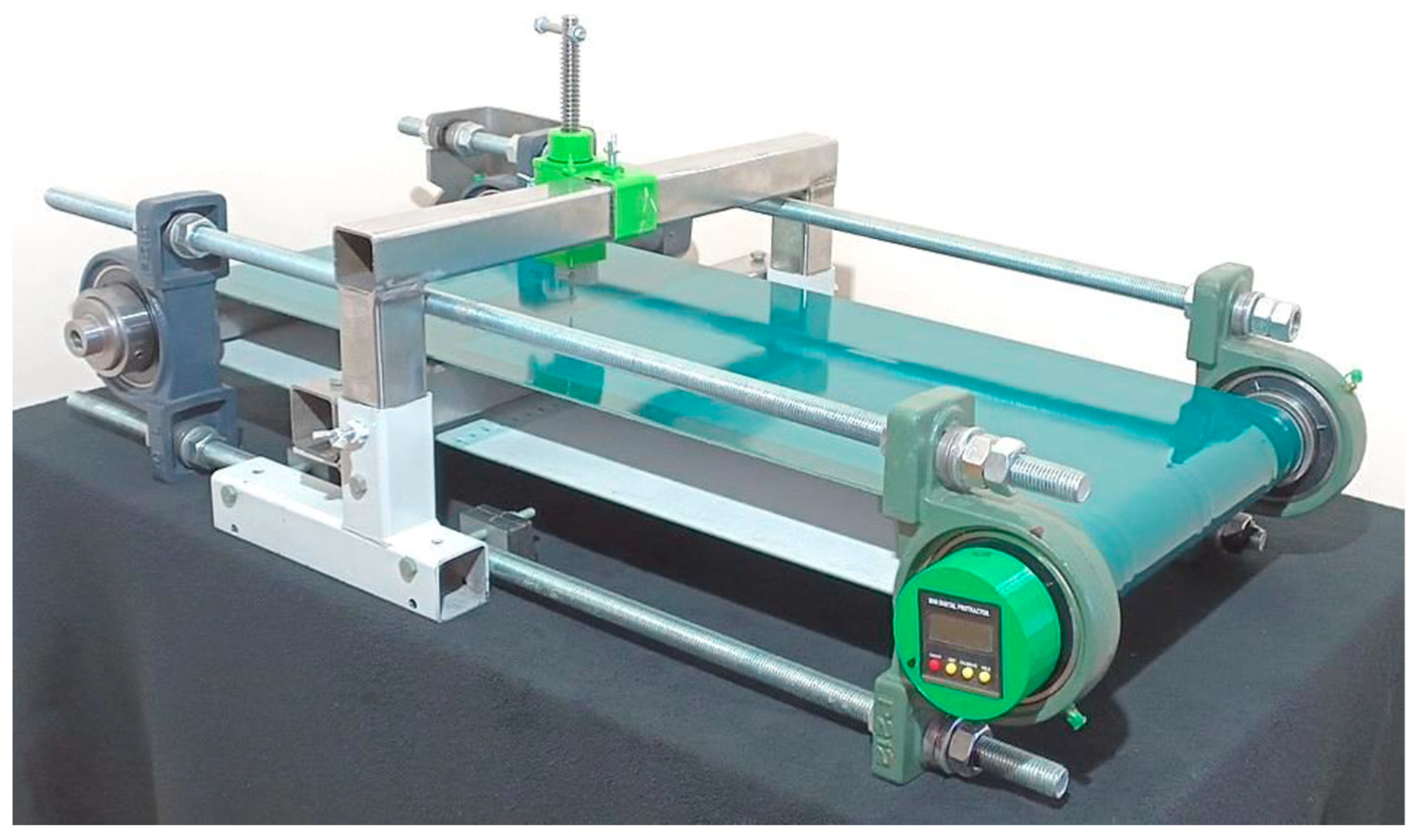
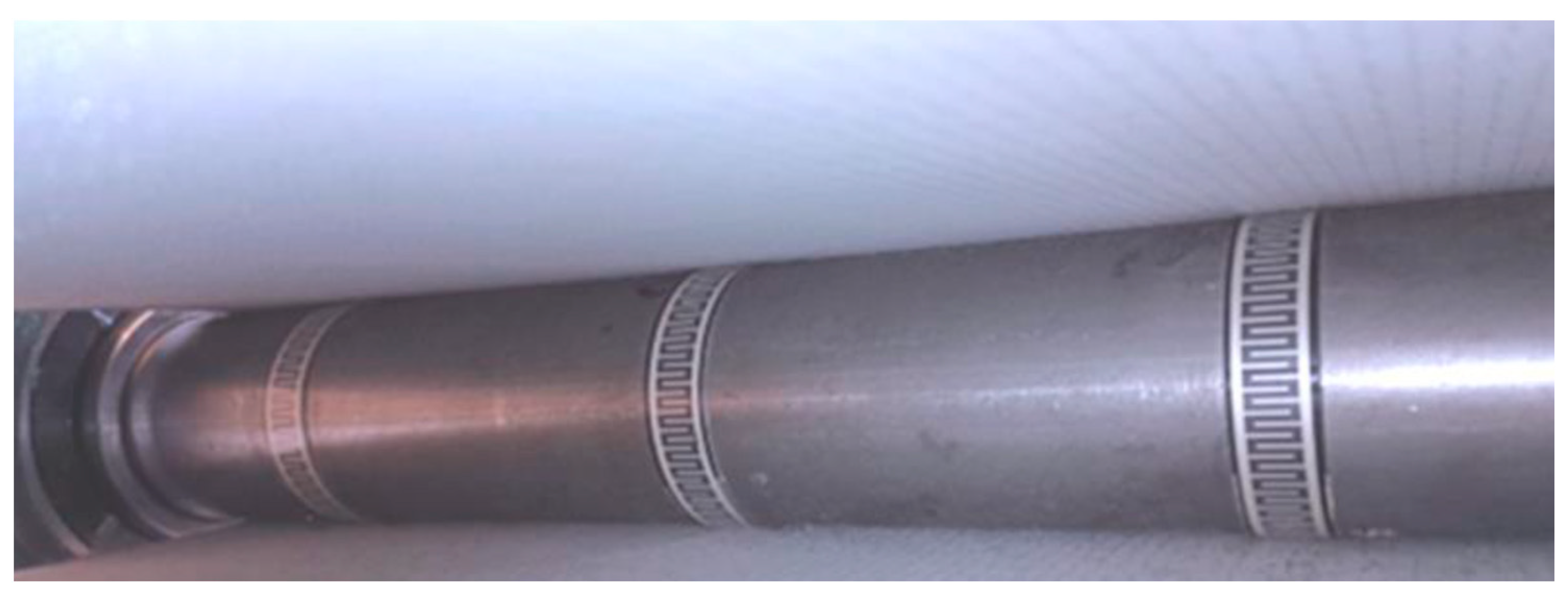
The research standing on which the measurements were carried out was a model of a belt conveyor, shown in Figure 5. Its supporting structure consists of four bearing units with self-aligning ball bearings, and two drums are mounted in the inner races: a drive drum and a return drum, on which strain gauges T1, T2, and T3 are located.

Inside the return drum of the conveyor, there are elements of the measuring system, and on its surface, at a distance of lo = 100 mm from each other, as shown in Figure 6, three strain gauges are placed, which are the most important element of the measuring system. The return drum is mounted in two bearing units with self-aligning bearings, twisted in the same way as in the case of the drive drum.

Pinstripe thin-film strain gauge sensors DFRobot RP-L-170 with a thickness of t_t1 = 0.35 mm, a width of w_t1 = 15 mm, and a length of the measuring part l_t1 = 170 mm were used. The operating principle of these sensors is based on resistance change. When pressure is applied to the active area of the sensor, a connection is made in the conductive circuit, leading to a change in its resistance. Crucially, the output signal, expressed in ADU (analog-to-digital units), exhibits an inverse relationship with the applied pressure: as pressure increases, the ADU value decreases. This inverse characteristic is a key aspect for accurate data interpretation and conversion to physical force units. Three strain gauges, designated T1, T2, and T3, are precisely attached to the outer surface of the tail drum. They are strategically positioned at an equal distance of lo=100 mm from each other.

The measuring system includes an electronic circuit that converts analog data from one of the three strain gauge sensors, marked T1, T2, and T3, into a digital signal. The digital signal is sent via a Bluetooth module to the Terminal program for communication and data recording. The electronic system consists of a printed circuit board powered by 4.5 V, which contains a microcontroller with a built-in analog-to-digital converter.

The conveyor belt, the condition of which is to be monitored in real time on the test stand, is the most critical element of the conveyor. It rotates on two drums with a diameter of 60 mm, described above.

The experimental studies utilized two-ply, single-sided, welded conveyor belts. These belts featured upper covers and an adhesive layer made of polyvinyl chloride (PVC), while the internal fabric layers, forming the core, were made of polyester. This specific material combination is highly relevant due to PVC’s widespread industrial use, offering properties such as chemical resistance and mechanical strength, complemented by polyester’s textile properties that provide tensile strength and structural integrity.

The physical dimensions of the conveyor belt are as follows:

• Thickness 2 mm,
• Total length of the belt loop 1875 mm,
• Nominal width of the conveyor belt 350 mm,
• Multi-layer structure: top cover, ply (textile layer), inter-ply layer (adhesive/elastomeric), and bottom cover.

The mechanical properties and operating parameters are as follows:

• Tensile force for 1% pre-tension 8 N/mm,
• Drum diameter 60 mm,
• Operating temperature −10 to 88 °C.

The stand uses a controller that allows smooth adjustment of the motor’s rotational speed, thanks to which three speed values were checked for research purposes.

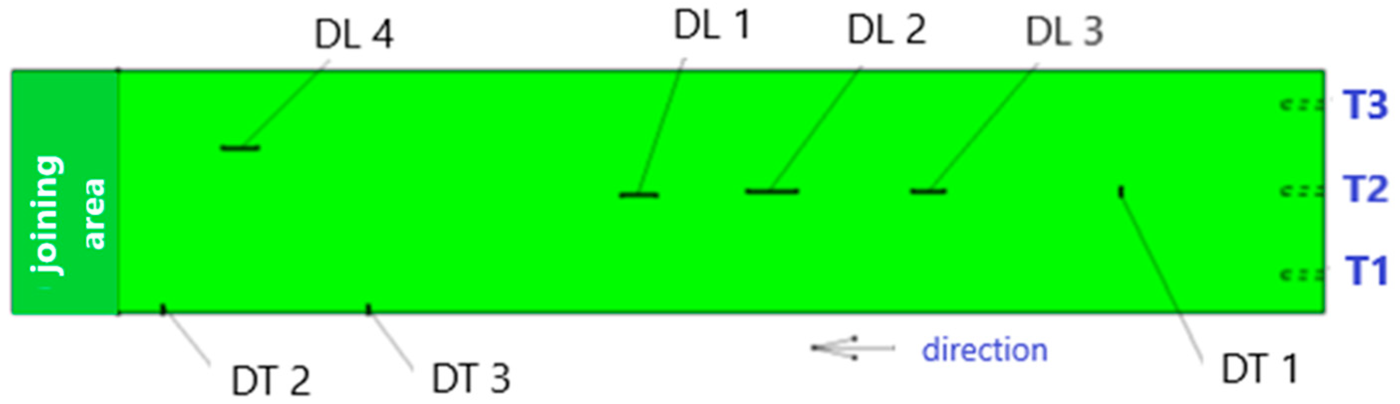
Notches and complete longitudinal and transverse cuts were made in the belt as stress concentrators, the presence of which causes crack propagation due to increased stress and belt destruction. In the research model, seven different damages were made on the conveyor belt (Figure 7). The description of the damages is included in

Table 1. Description of belt damages.

Type of Damage	Label	Description
Longitudinal damage I	DL1	Longitudinal cut of the strip 50 mm long, 170 mm from the edge (5 mm offset towards the strain gauge T1), 720 mm from the joint area
Longitudinal damage II	DL2	Longitudinal cut of the strip 70 mm long, 175 mm from the edge (in the axis of the strain gauge T2), 900 mm from the joint area
Longitudinal damage III	DL3	Longitudinal cut 45 mm long, 1 mm deep, 175 mm from the edge (in the middle of the strip), 1136 mm from the joint area
Longitudinal damage IV	DL4	Longitudinal cut 50 mm long, 1.5 mm deep, 115 mm from the edge (halfway between the strain gauges T2 and T3), 150 mm from the joint area
Transverse damage I	DT1	Cross cut 10 mm long, 170 mm to 180 mm from the edge (in the axis of the strain gauge T2), 1434 mm from the joint area
Transverse damage II	DT2	Cross cut 10 mm long, 0 mm to 10 mm from the edge (TI gauge side), 65 mm from the joint area
Transverse damage III	DT3	10 mm long cross section, 0 mm to 10 mm from the edge (TI gauge side), 359 mm from the joint area

.

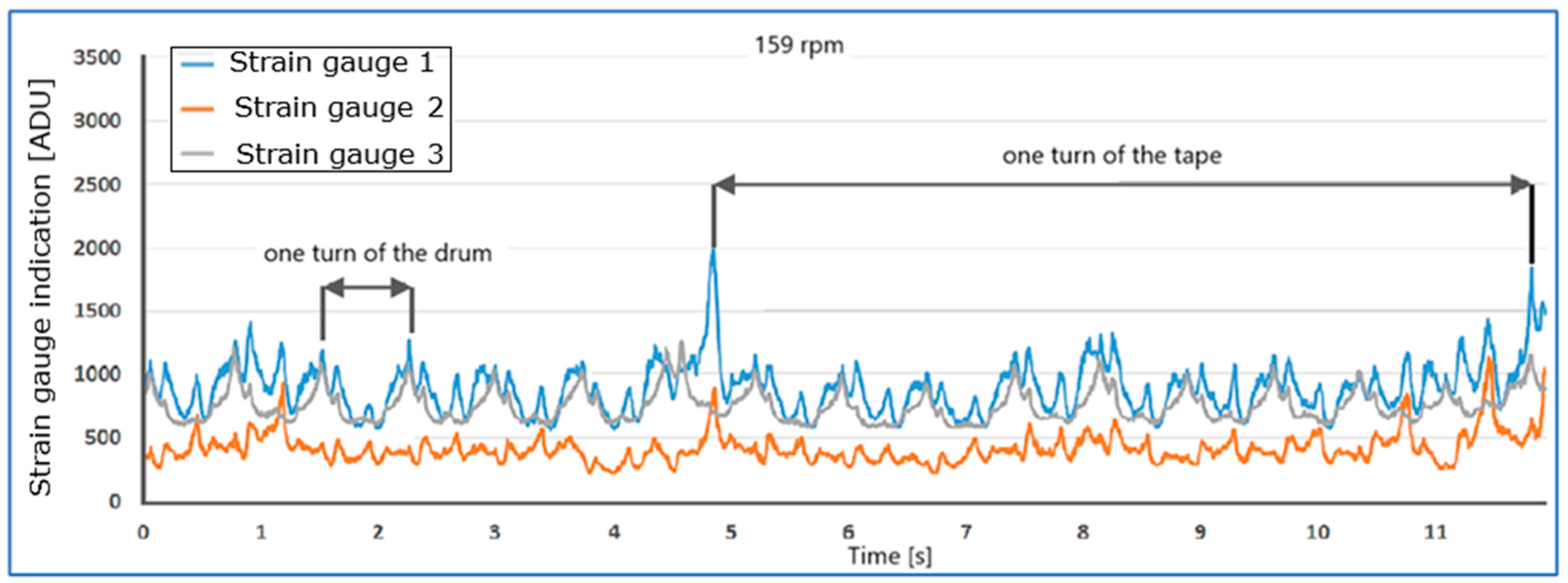
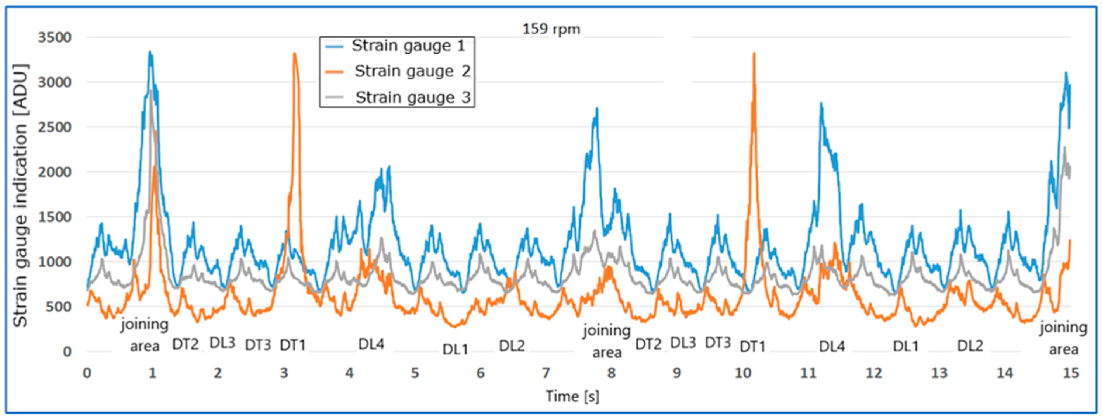
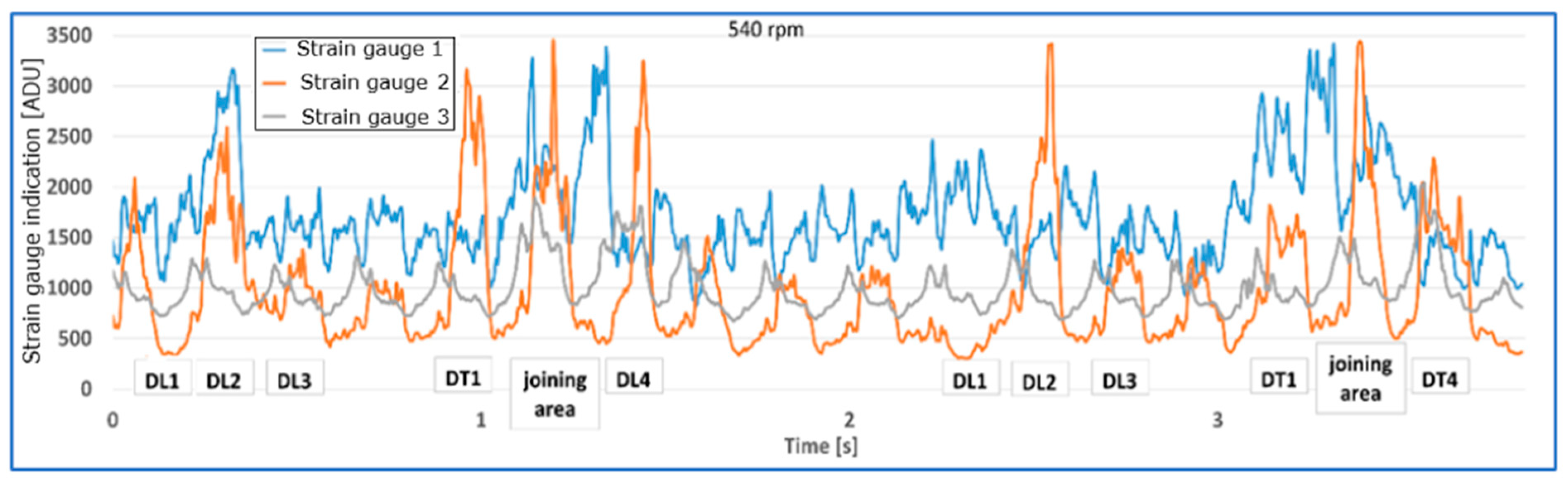
Figure 8 and Figure 9 show the waveforms of the readings of strain gauges T1, T2, and T3 of the unloaded belt at speeds of 159 rpm (Figure 8) and 540 rpm (Figure 9) as a function of time. The joining area of the tape is clearly visible on the waveforms. Figure 8 shows the rotation times of the drum and tape. The measurement results, obtained using an analog-to-digital converter, are presented in ADU (analog-to-digital units) as a result of analog-to-digital conversion.

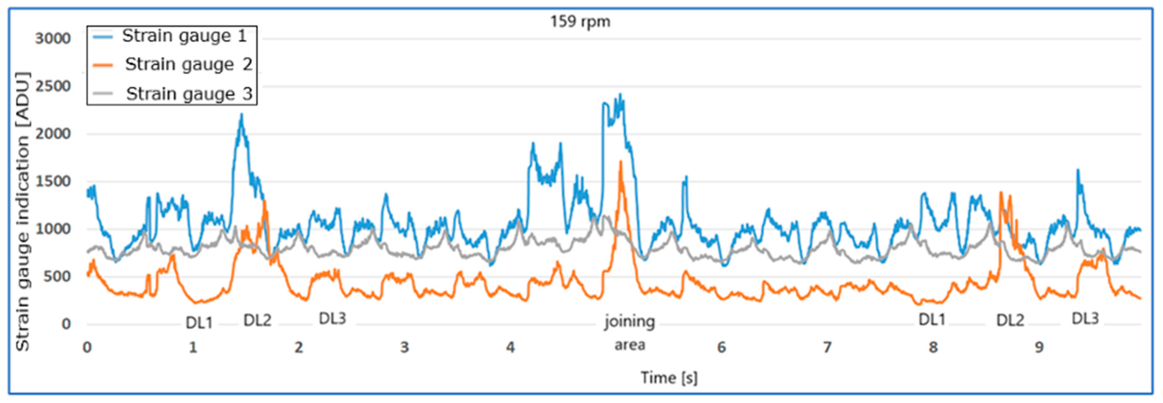
Figure 10, Figure 11 and Figure 12 show examples of strain gauge readings in the case of longitudinal and transverse belt damages for speeds of 159 rpm and 540 rpm.

Based on the conducted research, the following conclusions can be drawn:

• As the rotational speed of the drum increases, the damages generate an increase in the value of the readings, and the nature of the tension distribution on the individual strain gauges changes.
• Damages DL2, DL3, DL4, DT1 cause visible increases in strain gauge readings, most clearly visible by strain gauge T2.
• Damage DL1 generated a different tension distribution on the strain gauges than DL2, DL3, DL4, DT1, with strain gauge T2 being significantly more loaded.
• Two transverse cuts in the edge of the belt from the side of strain gauge T1, damages DT2 and DT3, caused an increase in the amplitude of the value and a decrease in the belt tension. The signal waveform for the damaged belt in relation to the belt without edge damage is anomalous. Under dynamic test conditions, the belt began to converge, immobilizing the conveyor and thus preventing further measurement and reading of results. An immediate stop of the conveyor would be advisable. The strain gauge readings indicate a decrease in belt pressure, which is especially visible for strain gauge T1, which is closest to damages DT2 and DT3.

The above qualitative analysis of the signals allows us to hypothesize that conveyor belt damages cause anomalies in the signals recorded by the strain gauges. Further activities aim to automatically detect these anomalies in order to locate the damage.

3. Results and Discussion

The TimeGAN network used for augmentation of healthy data consists of three main components: an encoder, a generator (decoder), and a discriminator. Each of these modules has its own layer structure, adapted to its function. The encoder, composed of three layers, transforms the input time sequences into a representation in the latent space, using an input layer to receive data, an LSTM layer with 128 units to model temporal dependencies, and a fully connected layer with a dimension of 24 to encode information in the form of a latent vector.

The generator (decoder) has a similar structure and consists of an input layer, an LSTM layer with 128 units, and a fully connected layer that transforms the encoded data into synthetic time sequences with the same number of features as the real data. The discriminator, on the other hand, is responsible for evaluating the authenticity of the generated samples and consists of four layers: an input layer, an LSTM layer with 128 units, a fully connected layer, and a sigmoid activation layer, which returns the probability that a given sample comes from the real dataset. The Recovery layer is not explicitly defined as a separate component. In this implementation, the Recovery function is taken over by the generator, which reconstructs the time data based on the latent vector. This configuration is possible because TimeGAN combines the features of a GAN and an autoencoder. In this role, the generator not only creates synthetic data but also reconstructs real sequences, which is sufficient for learning temporal representations and their realistic reconstruction.

In total, the entire TimeGAN network consists of 10 layers and uses an architecture based on recurrent neural networks, which enables effective modeling of complex temporal dependencies in data and generating realistic sequences.

For samples with damages, the system responses to local longitudinal and transverse tape damages were separated. Then, using Equation (1) and changing the gain $k_i$ and offset, the system’s responses to damages of various sizes and locations were obtained. In this way, a set of runs with tape damages of various sizes and locations and in various configurations was obtained.

The architecture of the LSTM network consists of 14 layers. It includes an input layer with dimensions of 1xData Sequence Length x 3 channels (corresponding to three strain gauges). The network contains two downsampling blocks, each including a 1D convolution, ReLU activation, and dropout layers. In addition, there are two upsampling blocks that use 1D transposed convolution, ReLU activation, and dropout layers. To ensure that the output sequences retain the same number of channels as the input, a 1D transposed convolution layer should be included, with the number of filters corresponding to the number of input channels.

The modification of the algorithm consisted of adding an attention mechanism to the LSTM network. The attention mechanism was implemented by adding two fully connected layers that calculate the so-called attention score for each time step. These scores are then normalized by a SoftMax function, which allows assigning appropriate weights to the hidden states of the LSTM. The resulting context vector, which is a combination of states weighted by the attention mechanism, replaces the traditional approach of using only the last LSTM state.

Additionally, another LSTM layer was added after the attention layer to allow further processing of the already optimized signal. Transposed convolutional layers were used in the decoder to reconstruct the signal waveform based on the obtained context vector. Thanks to these modifications, the model more effectively reconstructs time signals and better detects important patterns, improving interpretation and accuracy of anomaly detection.

The data are pre-processed, which consists of synchronization, denoising, detrending, and normalization.

The models are trained on datasets without damages. A set after augmentation consisting of 1200 samples was used for training, which was divided into a training part (80–960) and a validation part (20–240 samples). The model was tested using validation data.

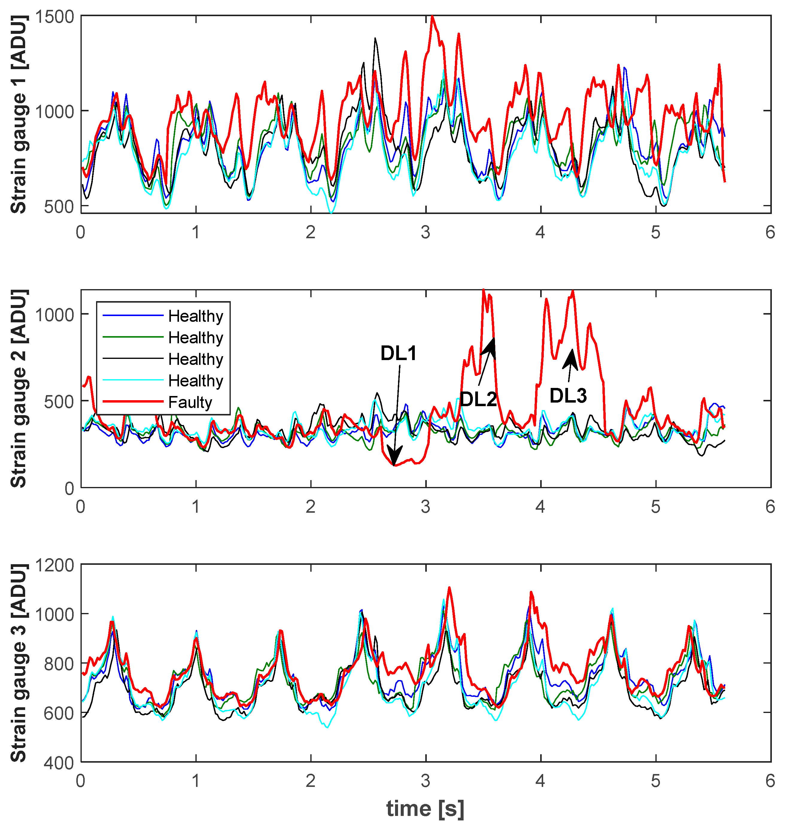
Detection of damages and their location is shown on the example of a real run with three longitudinal damages DL1, DL2, and DL3. Figure 13 shows synchronized indications of strain gauges as a function of time for four runs without damages and one with three longitudinal tape damages (DL1, DL2, DL3). Signal anomalies are most visible for strain gauge T2, although the remaining two also differ from the runs without damages.

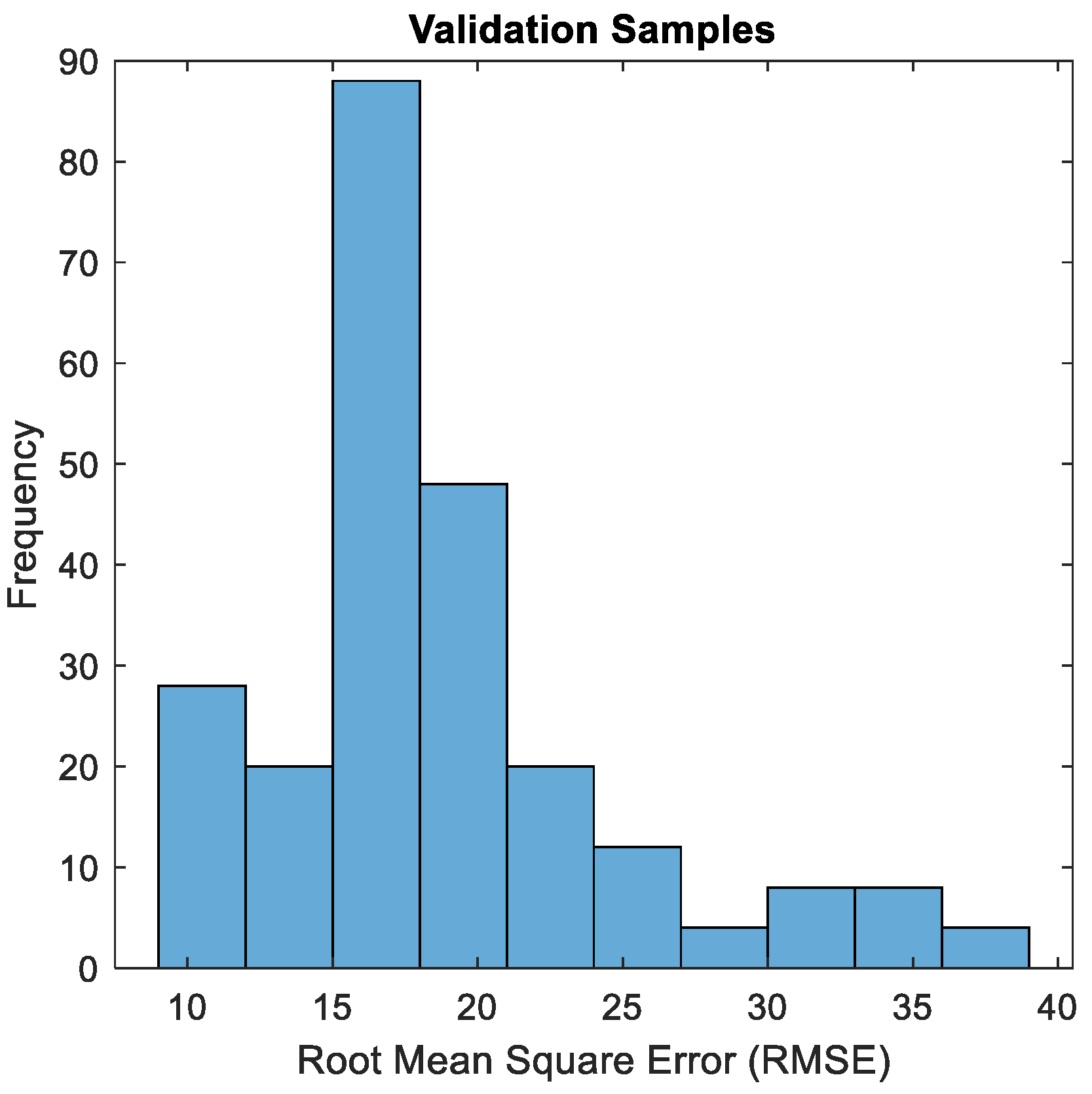
The described LSTM-AM model was used to reconstruct the signal. For each test sequence, the root mean squared error (RMSE) was calculated between the predicted and actual waveforms. The results are shown in the histogram (Figure 14).

A maximum RMSE of 38.8 ADU was obtained. This is also the limit of the RMSE value above which the runs are characterized by an anomaly.

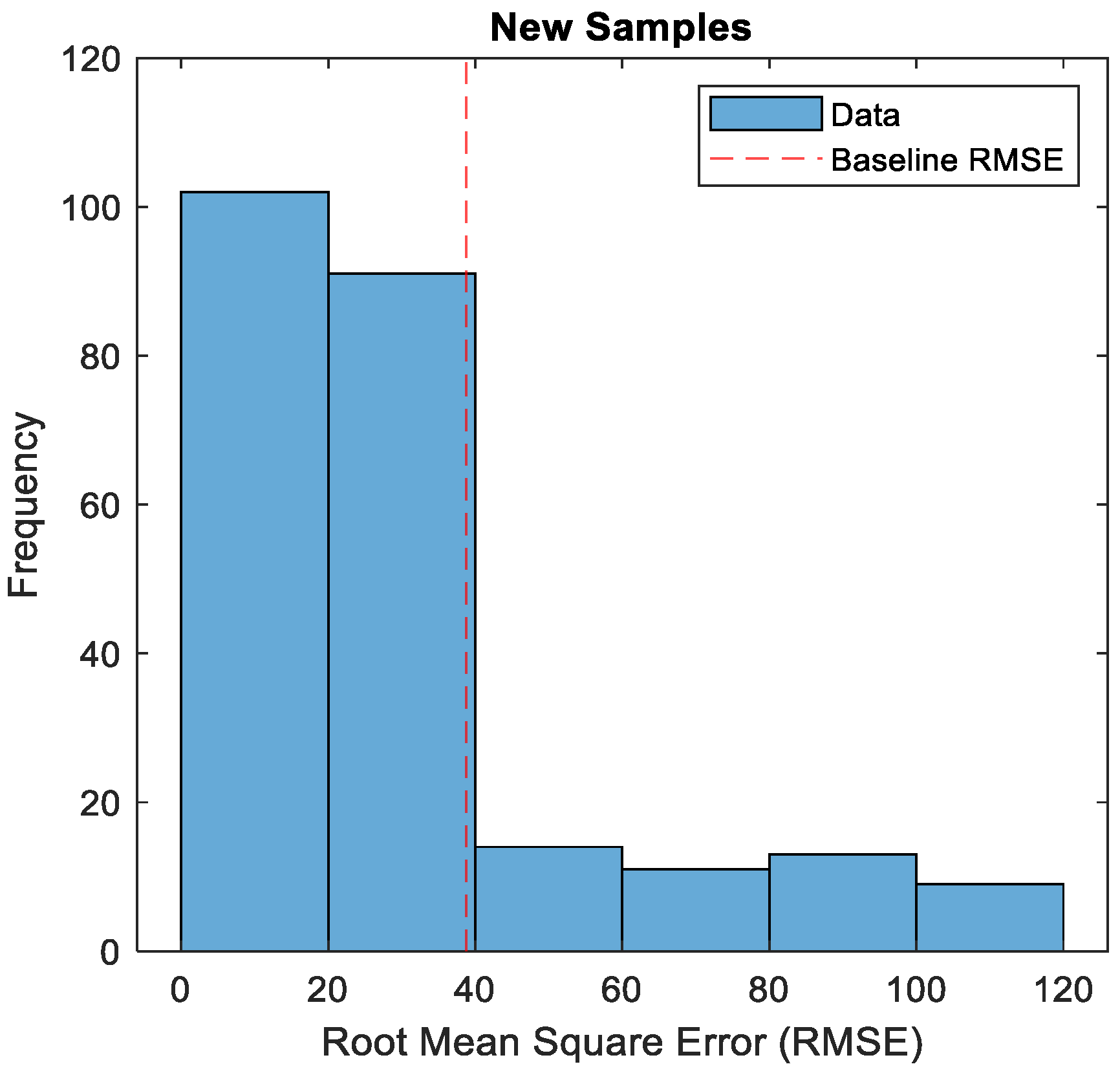
In the next step, 50 samples of the test set were replaced with damaged ones. RMSE was calculated again. The histogram with the marked maximum RMSE value is shown in Figure 15.

All samples with an RMSE value above 38.8 are considered anomalous. Their number is approximately equal to 50, which is the number of damaged samples.

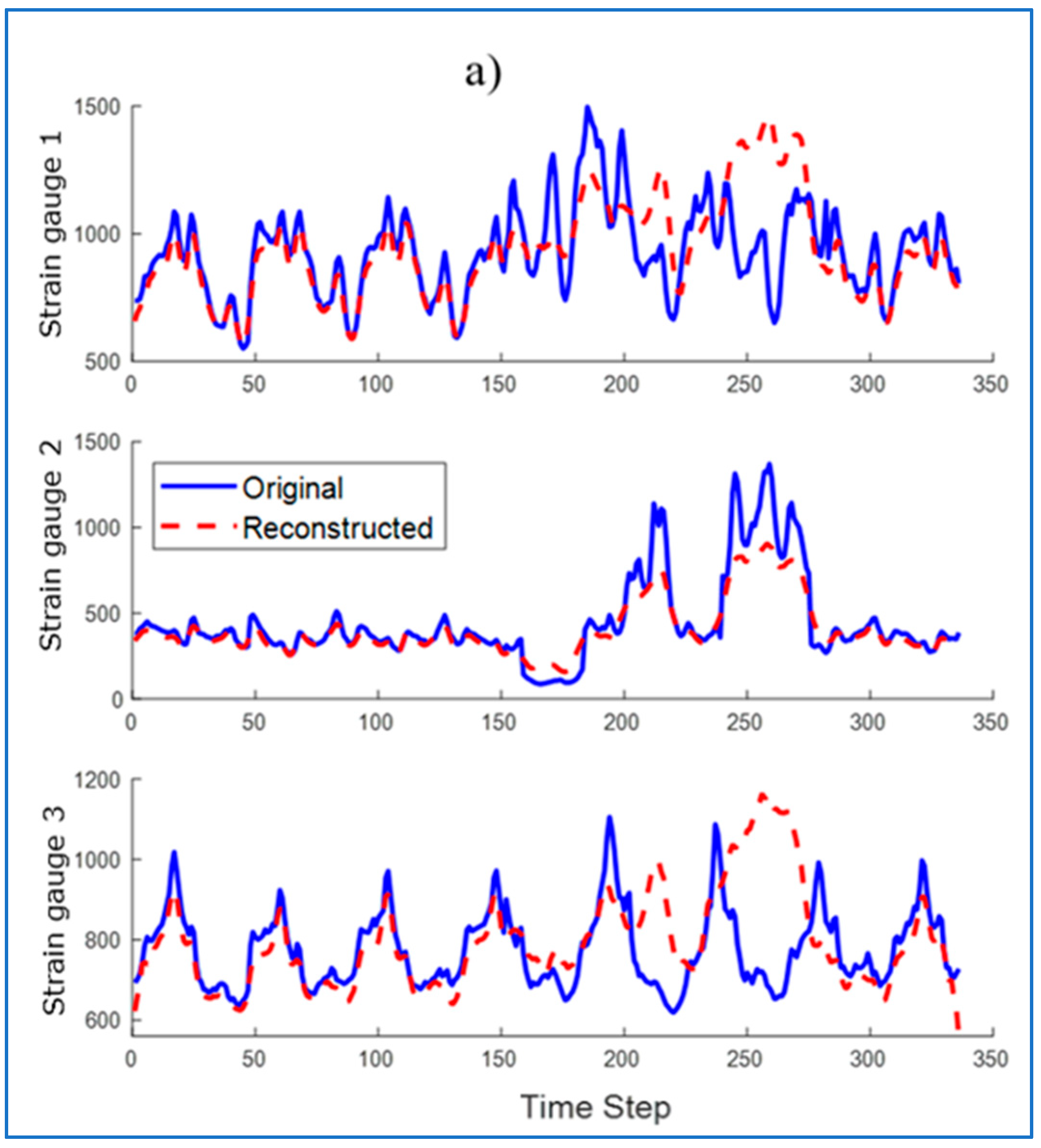
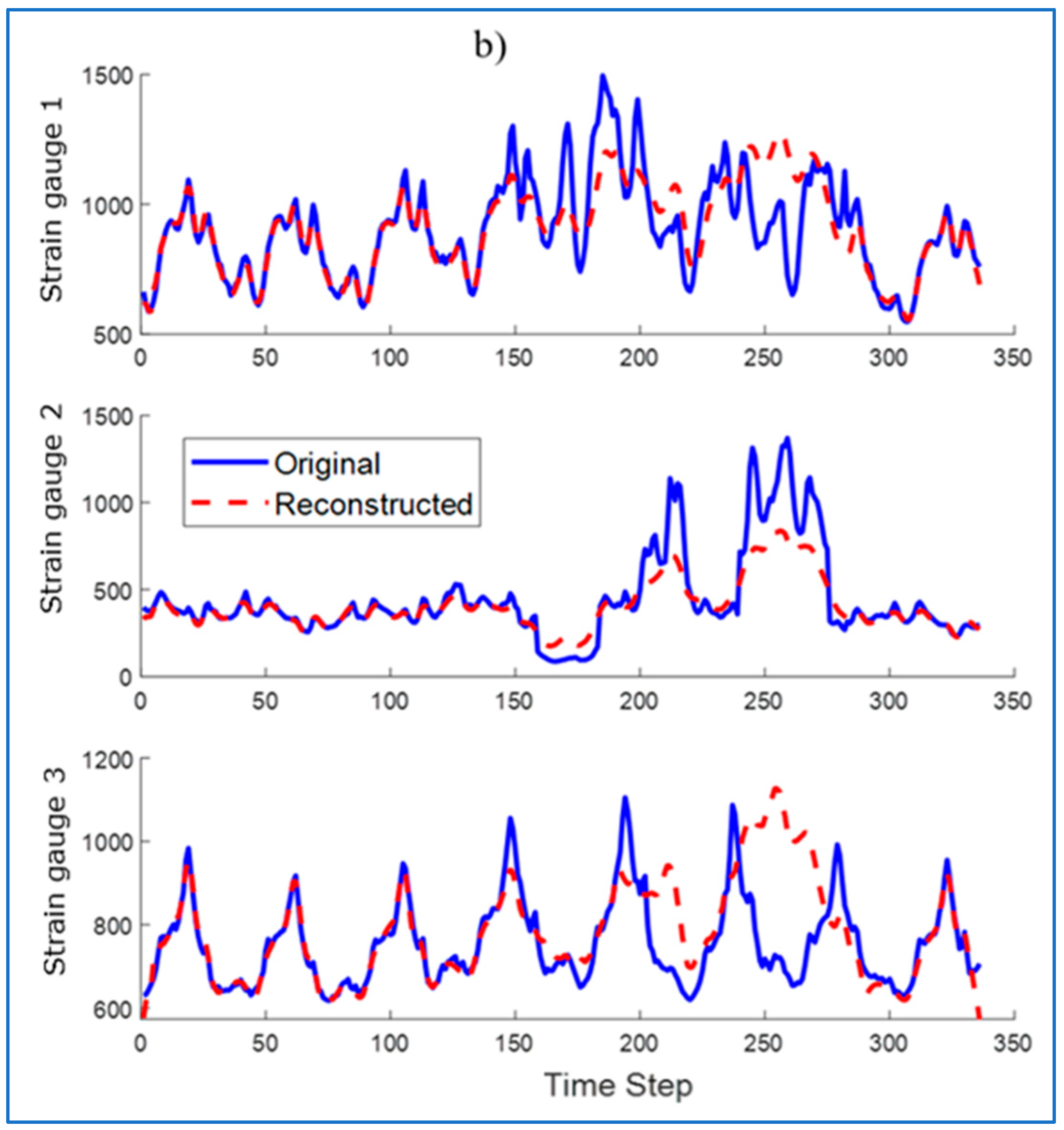
Then, the run was reconstructed by the LSTM network trained only on healthy samples. The reconstruction was performed using the LSTM network (Figure 16a) and using the LSTM-AM network (Figure 16b). Their waveforms were plotted on the original waveforms of strain gauge signals with damages.

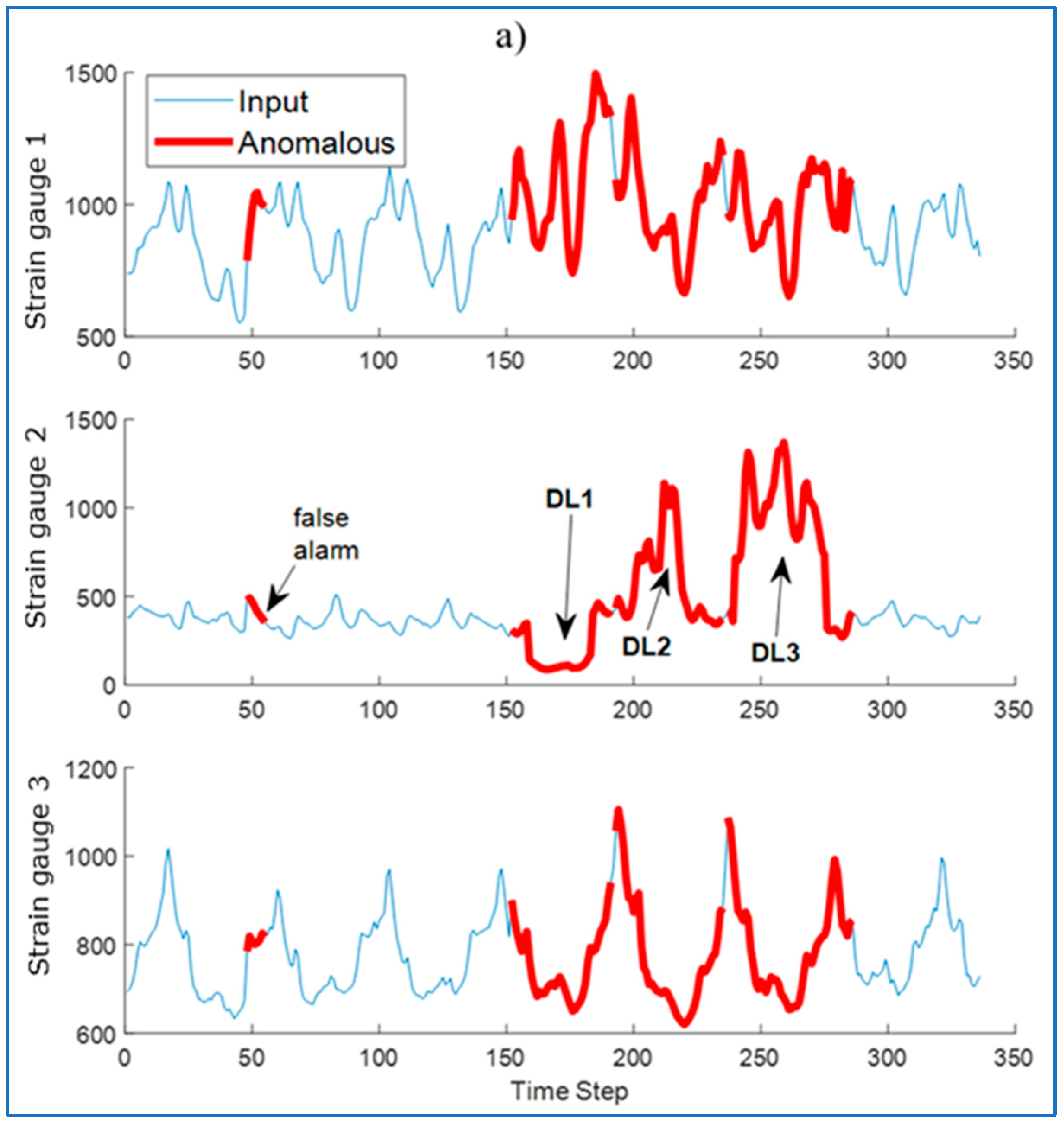
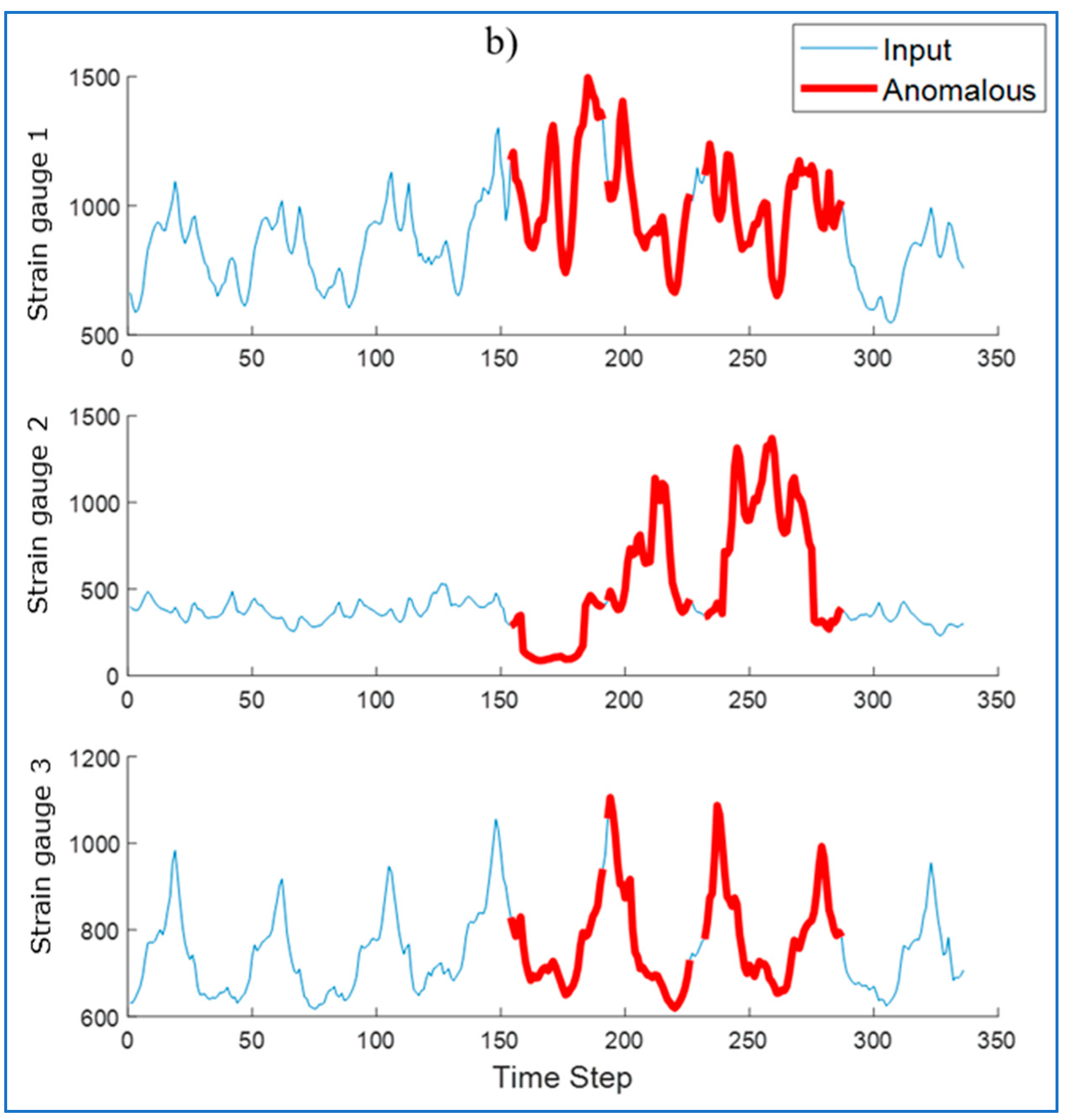
To detect anomalies in the sequence, the RMSE was determined between the input sequence (original) and the reconstructed sequence. Identified anomalies are windows that contain data with values at least 10% above the maximum RMSE error value. Areas recognized by the algorithm as anomalies are marked in Figure 17.

For some waveforms, areas incorrectly recognized as anomalies appear (Figure 17a—false alarm). The use of an attention mechanism allows to eliminate this phenomenon. The modification allows the model to better understand the context of the data, reduce noise, and thus allows the LSTM network to focus on the most important fragments of the input data, ignoring less important information. Thanks to this, the model can better identify real anomalies, and not normal deviations in the data.

Another method to eliminate false alarms is to check whether they appear regularly in subsequent runs. However, some small single anomalies may not be detected by the algorithm.

Next, for the LSTM and LSTM-AM models, the indicators used to evaluate the anomaly detection model were determined: accuracy, recall, precision, and F1-score (

Table 2. Model evaluation indicators.

Indicator	Value
	LSTM	LSTM-AM
Accuracy	94%	96%
Recall	90%	94%
Precision	84%	90%
F1-score	87%	92%

).

All false positive (FP) cases were reviewed and it turned out that for the LSTM model, fragments such as in Figure 17a have an impact on this. The method to eliminate them is to check whether they appear regularly in subsequent runs. Another way is to reduce the detection sensitivity of the model by increasing the anomaly detection threshold (currently 110% RMSE max value). The LSTM-AM model is free of this defect.

After reviewing all false negative (FN) cases, it turned out that these are most often cases of a single longitudinal damage of the DL1 type or other single damages, where the response of the strain gauge system does not significantly differ from the response for the system without damages. Of course, the selection of the set of damaged samples has an impact on the results of the model evaluation indicators in Table 2.

To minimize anomaly detection errors, the measuring path should be calibrated regularly. The strain gauge sensors inherently possess general limitations, including restricted directional measurement, environmental sensitivity, susceptibility to overload, nonlinearity, surface finish requirements, calibration demands, and potential for interference. A more comprehensive discussion of these issues has been presented in one of the authors’ doctoral research papers [31] and further detailed in a separate publication [19]. Therefore, this topic is not the primary focus of the present work.

In the current study, these limitations were mitigated through a controlled experimental setup and robust data preprocessing steps. The research was conducted on a “test stand” (a conveyor model), which provided a controlled environment, significantly reducing external environmental interference during data acquisition. The described application concentrates on detecting and localizing mechanical damage (cuts, cracks) by analyzing changes in strain, an area where strain gauges prove highly effective. The concern regarding limited directional measurement is addressed by the strategic placement of three strain gauges (T1, T2, T3) on the drum to effectively capture changes in stress distribution. Furthermore, the collected data underwent extensive preprocessing, which included synchronization, denoising, detrending, and normalization. These steps are crucial for alleviating noise, nonlinearity, and environmental influences, ensuring the high quality of data fed into the deep learning model.

The presented method allows to locate the damage. With a known tape speed, the distance of the damage area from the beginning of the tape can be determined.

4. Conclusions and Future Work

In the conducted studies, a novel method for detecting and localizing conveyor belt damages was presented, utilizing the LSTM-AM neural network and a hybrid data augmentation method. The results showed that using the TimeGAN model to generate synthetic data for undamaged cases, along with a superposition of one-dimensional observation sequences for augmenting damage data, effectively increased the number of training samples, which translated into improved model performance. The LSTM-AM model accurately identified anomalies in strain gauge signals, allowing for precise localization of damages. Analysis of the results revealed that the largest signal changes occurred in strain gauge T2, particularly in cases of DL2, DL3, DL4, and DT1 damages. Incorporating an attention mechanism into the LSTM network reduced the number of false alarms, thereby enhancing both precision and recall compared to the traditional LSTM version. RMSE error histograms confirmed the model’s effectiveness in detecting damages. Signal reconstruction by the LSTM-AM model more accurately reproduced the original waveforms than the standard LSTM, significantly enhancing detection accuracy. Additionally, DT2 and DT3 damages at the belt edge caused a reduction in tension and destabilization of the conveyor’s operation, which could lead to its stoppage.

The presented solution represents a significant advancement in conveyor belt diagnostics, offering a holistic approach to early damage detection and improved operational reliability. Its uniqueness lies in the synergistic integration of key innovations:

• Hybrid data augmentation effectively overcomes the fundamental problem of fault data scarcity, enabling the efficient training of robust deep learning models.
• The cost-effective strain gauge system provides continuous, precise real-time measurements of loads and stresses, standing out for its low implementation and operational costs. Its main advantage is eliminating the need for structural intervention in the belt or stopping the conveyor, which allows for the early detection of subtle changes signaling belt deformation, pulley misalignment, or uneven wear.
• Precise real-time damage localization, particularly in textile belts, fills a significant gap in existing methods.
• The LSTM network with an attention mechanism (LSTM-AM) enhances system robustness, improving detection accuracy and reducing false alarms in complex time series data.

It is important to emphasize that while the strain gauge system does not directly measure belt thickness or provide the same precision in tear localization as more expensive ultrasonic or laser methods, its strength lies in acting as an effective and budget-friendly early warning tool. It enables immediate anomaly detection, allowing for preventative measures to be taken before a minor issue escalates into a major failure or unplanned downtime. The ability to prevent “destabilization” and “stoppage” is direct evidence of the system’s proactive nature in averting serious operational consequences.

The current study primarily focused on a specific type of conveyor belt, a welded PVC (polyvinyl chloride) and textile core conveyor belt, within a controlled laboratory setting. While the underlying principles of strain gauge monitoring, hybrid data augmentation, and LSTM-AM for time-series anomaly detection have yielded good results, the direct transferability of the trained model to drastically different belt materials, constructions, or operational environments requires further investigation. Several factors contribute to these applicability challenges. One such factor is material properties. Different conveyor belt materials, such as rubber, steel cord, or various fabric plies, exhibit distinct mechanical properties, including stiffness and damping characteristics. These differences will significantly alter how damages propagate and how strain gauges respond to those damages. The current model’s learned patterns are specific to the mechanical response of the PVC and textile core belt.

Further research will concentrate on optimizing the model for various belt types and enhancing the system with additional sensors to further improve damage detection effectiveness. It is also crucial to accurately model the response to localized damage to generate precise synthetic data. In the next phase, different methods of signal reconstruction using deep learning algorithms will be compared.