Abstract
Accurate and robust detection of fabric defects under noisy conditions is a major challenge in textile quality control systems. To address this issue, we introduce a new model called the Logarithmic Deep Residual Shrinkage Network (Log-DRSN), which integrates a deep attention module. Unlike standard residual shrinkage networks, the proposed Log-DRSN applies logarithmic transformation to improve resistance to noise, particularly in cases with subtle defect features. The model is trained and tested on both clean and artificially noised images to mimic real-world manufacturing conditions. The experimental results reveal that Log-DRSN achieves superior accuracy and robustness compared to the classical DRSN, with performance scores of 0.9917 on noiseless data and 0.9640 on noisy data, whereas the classical DRSN achieves 0.9686 and 0.9548, respectively. Despite its improved performance, the Log-DRSN introduces only a slight increase in computation time. These findings highlight the model’s potential for practical deployment in automated fabric defect inspection.
1. Introduction
Defects in the fabric rolls that machines produce are very typical in the textile industry. All diagnostic applications used in the industry are included in the quality control system. Quality control is crucial for lowering costs and enhancing the final product. Maintaining the quality control process manually takes time and is ineffective because everyone doing the control identifies the errors based on their personal experiences. Additionally, it is improbable that the investigator will be able to find all the flaws because of the possibility that they will miss some of them. Quality control should be carried out automatically for the reasons listed above as well as the fact that quality is crucial to the textile industry. There are numerous studies in the literature to diagnose fabric faults.
A technique to find fabric faults that could happen during fabric manufacturing on knitting machines was developed by Hanbay et al. [1]. In the dataset, they used 5923 defective images and 3242 poor ones. Filtering, feature extraction, and classification using artificial neural network (ANN) were the processes used. The performance of fabric fault classification was 90% [1]. However, their approach relied heavily on manual feature extraction and lacks adaptability to complex or noisy environments, limiting real-world applicability. In contrast, our method performs automatic deep feature learning and is designed to be robust against noise. A method for the automatic localization and classification of flaws in yarn-dyed fabrics was reported by Zhang et al. [2] and is based on YOLOV2. First, 276 images of defects in yarn-dyed fabrics were gathered and prepared before labeling. While effective for localization, YOLOv2 is primarily designed for general object detection and may not sufficiently capture subtle texture-based defects in fabrics. Our approach focuses on enhancing sensitivity to fine-grained defect patterns. A quicker multi-channel RCNN is another tool used in the detection of fabric defects [3]. To detect fabric defects, geometric data augmentation and generative adversarial network (GAN)-based data augmentation were employed to supplement the training examples in [3]. The proposed method significantly outperforms the traditional fast- region convolutional neural network (Fast-RCNN) in simulation. With the Fast-RCNN augmented dataset, the recommended multi-channel average accuracy has increased to 90.05%. Although data augmentation techniques help expand training data, and they do not inherently address robustness to real-world noise. Unlike this work, our model integrates noise robustness directly into its architecture. Liu et al. [4] classified fabric defects using artificial neural networks. The accuracy rate was determined to be 99%. Fabric defects were classified using U-Net, a convolution neural network (CNN) approach. Similarly to [1], this method uses shallow architectures that may not generalize well across varying fabric types or noisy backgrounds. Our model leverages a deeper structure with residual and attention mechanisms to overcome such limitations. In another study, they proposed a deep architecture for detecting fabric defects in real time during production [5]. They were 99% accurate. Although U-Net offers strong segmentation performance, it is computationally intensive and primarily suited for pixel-wise segmentation. Our model, on the other hand, offers a classification solution that balances accuracy and computational efficiency. Lu et al. [6] proposed defect transfer, a highly contentious data augmentation method. The location and size of a defect in network training did not fully depend on the background texture because the defect could be anywhere on a background texture of any size. With only 1% fabric defect data in the ZJU-Leaper dataset, the method achieved comparable performance to the most recent fabric defect classification methods. This approach introduces novelty in data augmentation but still depends on synthetic data distribution. Our method addresses variability directly through architecture, without relying solely on artificial augmentation. However, most of these methods rely heavily on clean training data or extensive data augmentation strategies, and they tend to degrade under real-world noisy conditions.
Fang et al. [7] used haptic sensors on a robotic arm to automate and standardize data collection and create fabric datasets. In addition, to detect fabric types, an integrated CNN with an attention mechanism in the channel domain has been developed. This method improves data collection and introduces attention, which is aligned with our use of attention modules. However, we extend this concept by incorporating logarithmic shrinkage to enhance noise robustness. Shao et al. [8] proposed a semi-supervised structure error detection method that is pixel-by-pixel combined with a multitasking (MT) averaging tutorial. To improve defect segmentation, a multitasking detection model was created by utilizing its supplementary information for fault area detection, fault contour detection, and fault distance map detection. While multitasking can boost performance by learning auxiliary tasks, it increases model complexity. Our model remains efficient while achieving robustness through its shrinkage mechanism. Khodier et al. [9] used and tested several deep-learning models for unsupervised defect detection, including image preprocessing and CNNs. Furthermore, multispectral imaging, combining normal red–green–blue (RGB) and near-infrared (NIR) imaging, was implemented to improve and increase the accuracy of our system. The proposed method by EfficientNet CNN provided high accuracy, reaching approximately 99%. Multispectral imaging improves detection but adds hardware complexity. Our work maintains high accuracy using only standard RGB images, which is more practical for real-world deployment. In another paper, an improved YOLOv4 algorithm for fabric defect detection with higher accuracy is proposed, employing a new structure based on SoftPool rather than MaxPool [10]. Experiment results show that, when compared to the original YOLOV4, the enhanced YOLOV4 increases mean average precision (mAP) by 6% while decreasing frame per second (FPS) by only 2%. Despite the promising accuracy values, these approaches often depend on complex architectures, additional modalities (e.g., multispectral or tactile data), or heavy computational resources, which limits their applicability in real-time or cost-sensitive industrial environments.
In another article, an improved YOLOv4 algorithm for fabric defect detection with higher accuracy is proposed, employing a new SPP structure based on SoftPool rather than MaxPool [11]. Experiment results show that, when compared to the original YOLOV4, the enhanced YOLOV4 increases mAP by 6% while decreasing FPS by only 2%. SoftPool enhances feature selection, but these models in [10,11] still operate under ideal imaging conditions. In contrast, our Log-DRSN explicitly targets noisy environments. Xia et al. [12] proposed an unsupervised and real-time two-stage framework for fabric defect detection. In the first stage, density maps were generated to identify abnormal regions, and in the second stage, defects were automatically classified based on these maps. Zhang et al. [13] enhanced the YOLOv5 network with an attention mechanism to improve accuracy and efficiency in fabric defect detection. The model was strengthened with a coordinate attention mechanism to more precisely localize defects. Their study achieved 96.9% accuracy and a 95.3% F1-score on a publicly available fabric defect dataset. The average maximum success rate of 87.94% was attained in [14], where spectral domain and spatial domain techniques were employed for fabric detection and classification. Statistical, morphological, fast Fourier transform (FFT), discrete cosine transforms (DCT), and Gabor and Wavelet transforms are among the methods employed. Although comprehensive in features, this approach does not leverage deep learning, limiting its adaptability. Our deep model learns features end-to-end without handcrafted transformations. With the VGG19 architecture, it has been utilized to identify fabric flaws [15]. The success rate achieved is 94.65%. This method uses a standard CNN architecture without specific modifications for defect detection or noise resilience. Our work introduces architectural changes (logarithmic shrinkage and attention) to address these issues. The success rates for detecting fabric flaws using the deep transfer learning approach were 95.53% and 93.82%, respectively, in Ref. [16], where InceptionV3 and DenseNet121 were utilized. These are powerful models but trained in a transfer learning setting that may not adapt well to fabric-specific noise. Our model is trained from scratch with fabric defect noise in mind. By using simple image processing approaches, Vladimir et al. [17] were able to detect and categorize fabric problems with a 95% success rate, which represents an improvement of 50% over manual defect detection. Although showing improvement over manual inspection, this method is outdated compared to modern deep learning techniques. Our method automates detection with state-of-the-art performance. To address these limitations, our proposed Logarithmic Deep Residual Shrinkage Network (Log-DRSN) incorporates a logarithmic mapping combined with residual shrinkage and attention mechanisms. This design improves robustness against noise without requiring additional sensor modalities or sacrificing computational efficiency, making it more suitable for practical textile inspection environments. Table 1 presents a comparative analysis of existing studies in the literature regarding fabric defect detection and classification.

Table 1.
A comparison of fabric defects detection and classification in literature.
In this study, a new deep learning-based model is created for categorizing fabric defects. We preferred to apply the RSN model to this problem thanks to the flexibility of the RSN model and the customizability of the RSN structure and parameters. In addition, the RSN architecture was chosen thanks to the advantages of having the ability to recognize and classify complex faults and the ability to detect the difference between normal and abnormal situations. The suggested deep attention-based logarithmic deep residual shrinkage network (Log-DRSN) model and the classical residual shrinkage network (RSN) model both use all the layers developed for the RSN model. For both models, all layers and parameters are identical. To experimentally test the suggested model, we produced our own dataset. In our dataset, there are four main kinds of fabric failures. Despite promising results, existing defect detection approaches often suffer from one or more limitations such as sensitivity to noise, reliance on handcrafted features, or poor generalizability across fabric types. These challenges significantly affect performance in practical industrial environments. To address these gaps, this study proposes a novel Logarithmic Deep Residual Shrinkage Network (Log-DRSN), which combines logarithmic transformation with adaptive shrinkage and attention mechanisms. This architecture aims to provide robustness against noise and improved generalization without the need for additional data modalities or extensive feature engineering.
The following are some of this study’s advantages and contributions:
- The proposed Log-DRSN model significantly improves classification accuracy on fabric defect detection, achieving up to 99.17% accuracy on noiseless data and demonstrating robust performance even with noisy inputs.
- The integration of a novel deep attention mechanism and logarithmic activation enhances feature learning, noise robustness, and model interpretability, while also reducing computational complexity compared to traditional activation functions.
- Extensive experimental validation confirms that the model offers superior performance and numerical stability, making it a promising tool for predictive maintenance in the textile industry.
2. Four-Point System in the Fabric Inspection
The four-point system is the method used to regulate fabric quality in the apparel sector. The process of preserving the quality of the raw materials utilized to produce the product is known as inspection. The Dallas system, the Graniteville 78 method, the 4-point system, and the 10-point system are typically used for fabric quality control [18,19,20,21]. However, the four-point system is realistic, impartial, and well-known across the world. In this system, based on the kind, severity, and amount of the defect, the expert defines criteria to assign penalty points ranging from one to four. An error might receive up to four penalty points. Significant faults are considered while measuring a fault’s width and length. Minor faults do not contribute to the penalty points. Fabric quality is graded in points per 100 m2. The total penalty points are calculated for the total faults found in a roll of fabric [22].
Table 2 illustrates the relationship between different types of faults and the corresponding penalty points assigned within the four-point system. This relationship is fundamental to the system’s ability to provide an objective and standardized assessment of fabric quality. The penalty points reflect not only nature but also the severity of defects, ensuring that more critical faults receive higher penalties. Minor imperfections, due to their negligible impact on fabric performance, are excluded from the penalty calculation. By quantifying defects in terms of penalty points per 100 square meters, the system facilitates a consistent evaluation of fabric quality across batches and suppliers, making it a widely accepted quality control method in the textile industry worldwide. Figure 1 demonstrates the various image-taking mechanisms employed in fabric inspection, which play a crucial role in automating defect detection and enhancing the accuracy of the quality control process.
Table 2.
Relationship between fault and penalty points in the four-point system. Fabric width (in inches) and defect size ranges (in mm2).
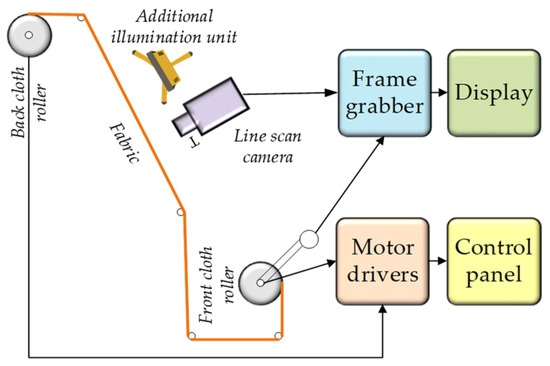
Figure 1.
Image-taking mechanisms are used in fabric inspection.
In Equation (1), the θ value is 100 square yards; the μ value is the total number of defect points; the β value is total fabric yardage; and the γ value is the width of the examined fabric.
3. Material and Methods
The classical DRSN model and the Log-DRSN model suggested in this research were generated to be used in the classification of fabric defects. Both models were investigated on open datasets that we created and that are commonly used in the literature [18,19,20,23,24,25,26,27,28,29,30], and the results are presented in comparison. Furthermore, Log-DRSN, a new model proposed in this study, was evaluated with both synthetic noise and noise-free data. The proposed method’s noise resistance was investigated.
3.1. Deep Residual Network (DRN)
The DRN is a custom neural network that aids in the handling of more complex deep learning tasks and models. As we design deeper networks, it becomes increasingly important to understand how adding layers can increase the network’s complexity and expressiveness. To reduce training errors, the Residual Network architecture (also known as ResNet) employs redundant blocks with multiple layers. The DRN employs the inter-layer redundant bypass connection method and proposes the concept of cross-layer identity mapping, allowing the number of network layers to be increased while the difficulty of model training is reduced. Figure 2 depicts a residual module from a two-layer network structure [23].
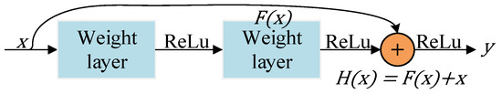
Figure 2.
A residual module.
The input property is represented by the parameter x in Figure 2, the nonlinear output of x, following double convolution, is indicated by F(x), the result of adding F(x) to the appropriate element of x is described by H(x), and the output result of H is expressed by the y value. If F(x) and x have the same dimensions, then y can be defined as
The activation function is represented by σ(x), which refers to the ReLU activation function, same as in (2). The size of must be adjusted if and have different dimensions for and to have the same dimensions, and then may be calculated as in (3):
To preserve the front features’ original appearance, this module uses the identity mapping method to introduce the front information. According to the experiments, the residual module efficiently lessens the model distortion brought on by the stacking of network layers in the neural network.
3.2. Generating Synthetic Noise
Due to the vibrations that take place during the acquisition of fabric images on the sliding band, there may be some noise in the images in the textile sector. The existence of this issue makes the classification procedure more difficult. The proposed method aims to be noise resistant as a result. The images in our dataset have synthetic noise added for this reason. In this investigation, noise types that are often utilized in the literature [24,25,26,27,28], namely Gaussian, Speckle, Poisson, and Salt and Pepper, were applied. For each type of noise, the effectiveness of Log-DRSN was evaluated independently.
3.3. The Recommended Method
The DRSN is an optimized version of the deep residual network [23]. This network can eliminate unnecessary noise [23]. The DRN is made up of three parts: the residual network, the attention mechanism, and the soft threshold function. Paying attention to unimportant features via the DRSN network’s attention mechanism and setting it to zero via the soft threshold function; in other words, the attention mechanism aims to pay attention to and retain important features via features. As a result, it enhances deep neural networks’ ability to extract useful features from noisy signals. The attention mechanism employs feature weighting to assign different weight values to each feature channel, resulting in a degree of sample noise reduction. The noise content of different regions in the same feature channel, on the other hand, varies. The attention mechanism’s limitation is that it cannot capture position information and feature weighting alone cannot meet the need for sample noise reduction. Unlike previous studies, this one introduced a new residual shrinkage network, Log-DRSN. The network’s computational power and success rate have both increased because of the Log-DRSN.
We enhance the attention mechanism to work more precisely and effectively, optimizing the training process of the model and ultimately yielding improved results. In contrast to the classical approach, our proposed model utilizes a logarithmic function in attention weights and attention output. This choice contributes to increased numerical stability by mitigating large differences between numbers. Unlike classical DRSN, it aids in expressing relative measures between features more accurately and better articulates errors in model predictions. The application of a logarithmic function to attention weights facilitates focused attention on a particular topic, especially when selecting from multiple attention topics in our model.
Another advantage of the Log-DRSN model is that, since a gradient-based optimizer is employed, the optimization algorithm proves to be more effective with the logarithmic function, delivering high performance. An additional consideration is that the Softmax function, when operating in large numbers, may introduce numerical stability issues, particularly in scenarios where calculating the probabilities of major and minor events is challenging. Using logarithmic functions helps stabilize calculations, reducing such problems and simplifying computations by converting the product of the logarithmic function and cross-entropy loss probabilities into addition. This streamlines the model optimization and learning processes. With incorporating new logarithmic function soft-thresholding and deep attention modules in Log-DRSN, the features the model needs to learn are suppressed. Unlike the classical approach, Log-DRSN demonstrates the ability to generalize using fewer parameters and exhibits faster learning. This leads to increased model accuracy and a reduction in over-fitting. Figure 3 illustrates the overall architecture of Log-DRSN, highlighting the flow of data through the initial convolutional layer, residual blocks with soft-thresholding, and the attention mechanisms. This schematic provides a clear visual summary of how the model integrates residual learning, adaptive feature suppression, and enhanced attention to improve fabric defect detection performance.
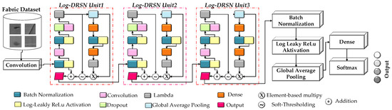
Figure 3.
The overview of Log-DRSN.
Operationally, the Log-DRSN model processes input images through a sequence of well-defined stages designed to enhance robustness and interpretability in noisy fabric defect detection scenarios. First, the raw input image is passed through an initial convolutional layer to extract low-level features. These are subsequently processed by a series of residual blocks that constitute the core of architecture. Each residual block contains two paths: a convolutional transformation path and an identity shortcut path, which collectively allow deeper training by mitigating gradient vanishing. Within these residual blocks, a soft-thresholding function is applied to suppress low-importance or noisy feature activations. This residual shrinkage mechanism adaptively filters irrelevant information, contributing to the model’s noise resistance. In parallel, an attention mechanism computes channel-wise weights by aggregating global contextual information and assigning higher importance to feature channels more indicative of defects. The model distinguishes itself by incorporating a logarithmic transformation into the attention computation. Unlike conventional attention that may suffer from numerical instability or overlook subtle differences between high- and low-activation regions, the logarithmic function stabilizes learning dynamics, dampens extreme activations, and facilitates nuanced feature discrimination. This mechanism enhances the attention module’s precision, especially when multiple defect-relevant patterns compete for representational priority. After the attention-weighted features are computed, the enhanced feature maps are forwarded through additional convolutional layers, followed by global average pooling and a fully connected classification layer. Moreover, the use of the logarithmic function within the loss function computation (via its interaction with cross-entropy loss) enables more efficient and stable optimization by transforming multiplicative terms into additive ones, thus improving convergence rates and reducing overfitting. In summary, the modular structure of Log-DRSN—comprising residual learning, adaptive shrinkage via soft thresholding, and enhanced logarithmic attention—not only allows the model to prioritize meaningful defect cues under real-world noise conditions but also ensures high classification performance with fewer parameters and faster training convergence.
3.3.1. Soft Thresholding
The idea is to use soft thresholding instead of feature weighting in DRSN. It is used to highlight features or reduce noise in noisy data. When you increase the threshold value to reduce the noise value, important features in the image may be lost. In addition, choosing a low threshold value can generate too many features and complicate the classification process. For these reasons, the optimal threshold value was selected through empirical tuning involving an iterative search process to effectively balance noise suppression and feature preservation.
Although the soft thresholding process does not explicitly distinguish between noise and small signals, it operates under the assumption that meaningful features typically manifest as stronger or spatially coherent activations, whereas noise tends to be random and less structured. This assumption guided the empirical tuning of the threshold parameter to achieve a balance between feature preservation and noise suppression.
3.3.2. Deep Attention Module
In recent years, the deep attention module has seen widespread use in the field of computer vision, particularly in image recognition [29]. More algorithms to incorporate attention mechanisms in neural networks have emerged with the emergence of deep learning. Figure 4 illustrates the deep attention mechanism employed in this study. This module generates various weight values based on the relevance of the feature channels, avoids model distortion by automatically learning the importance of each feature channel, and loads the correct weight values into the feature map. Feature weighting increases pertinent information in images while suppressing unimportant data. This module does not require the addition of new functionality or layers because of its straightforward structure and ease of deployment. Additionally, it has favorable traits in terms of computing complexity and model quality.
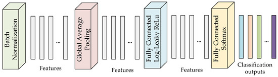
Figure 4.
Illustration of the deep attention mechanism in this study.
In this module, a set of one-dimensional vectors is produced by taking the absolute value of the output features and averaging it over each feature channel using global average pooling (GAP). One-dimensional vectors become a collection of normalized parameters after passing through the first fully connected layer (FC), batch normalization (BN), ReLU activation function, second fully connected layer, sigmoid function, and then element-wise multiplication with the appropriate elements [30]. The entire process, from the automatic adjustment of thresholds to the reduction in sample noise, is then performed by applying a soft threshold to each feature channel with the generated thresholds. The deep attention mechanism enables a model to concentrate on a specific region of an image. In tasks like object recognition or image classification, for example, the deep attention technique might let the model pay more attention to regions with crucial features and deliver more accurate results.
3.3.3. Log-Leaky ReLU Activation
Logarithmic approaches and computation-saving strategies like sparsity, pruning, and quantization have been suggested in the literature [31]. As the aggregation itself would become computationally expensive, the log-domain is used instead. The constant from the leaky ReLU function has been changed to in the log-leaky ReLU activation function [31]. As a result, a ReLU activation function in the log domain is obtained. It also has a single hyperparameter like the leaky-ReLU function. Figure 5 presents a mathematical illustration of the log-leaky ReLU activation function.
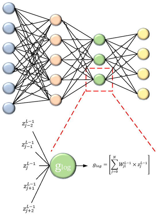
Figure 5.
Mathematical illustration of the log-leaky ReLU activation.
Here, is a sign parameter that takes binary values 0 or 1 and determines the behavior of the activation function accordingly. When , the function returns the input ; when , it returns . This parameter is initialized independently and controls the switching in the log-leaky ReLU formulation. The sign parameter can be initialized independently of the 0.5 value derived from the Bernoulli distribution and is chosen at random. This can be determined using the weights in the distribution used by the activation function’s magnitude value of (5). Equation (5) is derived from the recursive definition of the weighting function in the logarithmic activation framework. It defines the scaling behavior of at discrete points based on its values at . This ensures the preservation of logarithmic properties, contributing to numerical stability and smooth gradient propagation during training.
The Bernoulli distribution (0.5) and log sizes are sampled from the distribution in (6) since we are sampling from a normal distribution with a mean value of 0 and a standard deviation of . This means that the sampling parameters in the log domain are from a normal distribution [31]. The mathematical formulation in the Softmax layer is expressed as (7) and (8).
In the (8), δ is the back-propagation initiation term and is the only hot output label. Probability value calculation in log-domain is provided by (9)–(11).
To improve interpretability, we provide a visual comparison of ReLU, Leaky ReLU, and the proposed Log-Leaky ReLU in Figure 6. While ReLU outputs zero for negative values and Leaky ReLU allows small negative outputs, Log-Leaky ReLU introduces a logarithmic scaling that smoothly handles both positive and negative inputs, enhancing numerical stability and gradient flow. Log-Leaky ReLU logarithmically scales very small activations in the negative region, reducing issues like vanishing gradients. This enables more meaningful and balanced information flow in the negative domain during training. Additionally, the logarithmic growth for positive values prevents activations from becoming excessively large, further improving numerical stability. Thus, the model can learn more stably and precisely. The pseudocode of Log-DRSN is presented in Algorithm 1.
| Algorithm 1 Training of Log-DRSN |
| Input: training iterations, train size, batch size, each of training set , training sample of image, thresholding value, feature channel of , thresholding value of , width, height, Benoulli distribution, bias, collection of channels, j-th input features, scaling parameter, weight, and trainable parameters Output: j-th output feature map, j-th predicted label for do for do # compute feature maps # compute soft-thresholding # compute output feature # compute log-domain feature # compute log-domain softmax end for end for |
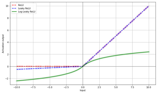
Figure 6.
Visual comparison of ReLU, Leaky ReLU, and proposed Log-Leaky ReLU activation functions.
4. Experimental Results
A new model based on deep learning was developed in this study, which was conducted for the classification of fabric defects. The generated model’s noise resistance was evaluated by manually adding a particular amount of noise to the data. Each technique in our investigation had the following hyper-parameter values: 0.001 learning rate, 32 batch sizes, 100 iterations, Adam optimization algorithm, and input pattern size normalized to 28 × 28 size.
4.1. Dataset Definition
In our dataset, there are images collected by the image acquisition mechanism of the fabric balls flowing over the sliding band. The dataset used in this study was custom-constructed for the purpose of evaluating the performance of the proposed Log-DRSN under realistic and noisy conditions. Figure 7 illustrates sample images along with their corresponding labels from our dataset, highlighting the diversity and complexity of defects present in the fabric samples. A total of 2500 training images were collected using a specialized image acquisition system positioned above the sliding band, where fabric balls are conveyed under controlled lighting and movement. The camera setup was calibrated to ensure consistent resolution and alignment across samples. Each image was altered during data augmentation by shifting it by 0.2, which corresponds to 20% of the image’s width and height, along the x and y axes., rotating it by 30 degrees, tilting it by 0.2, and enlarging it by 0.2 percent. The images are also rotated on a horizontal axis. The images in the dataset have Poisson, Gaussian, Speckle, and Salt and Pepper synthetic noises introduced. A total of 5% Gaussian noise was added. A random value is produced, and then Poisson noise is added. The mean and variance of speckle noise are 0 and 0.05, respectively. It was introduced with Salt and Pepper noise at a rate of 0.5.
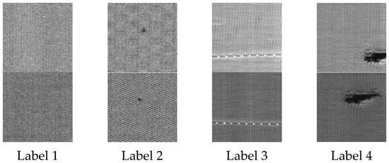
Figure 7.
Labels and sample images in our dataset.
4.2. Performance Comparisons of Proposed Method
The classical DRSN method in the literature and the Log-DRSN method we recommend consist of the same layer and parameters. Based on these findings, we may infer that Log-DRSN is an innovative, effective, and high-performance approach. Figure 8, Figure 9 and Figure 10 collectively demonstrate the comparative performance of the classical DRSN and the proposed Log-DRSN models under various noise conditions. Figure 8 shows the accuracy ratios of the classical DRSN when exposed to different noise types: Gaussian, Poisson, Speckle, and Salt and Pepper, highlighting the model’s varying robustness across noise environments. In contrast, Figure 9 presents the accuracy ratios of the Log-DRSN under the same noise conditions, illustrating its enhanced resilience and consistently higher accuracy compared to the classical approach. Figure 10 offers a direct comparison of both models’ accuracy rates across four scenarios, clearly demonstrating the superiority of the Log-DRSN in both noisy and noise-free settings. Although both models share identical architectures and parameter counts, with 336,260 trainable and 1376 non-trainable parameters in the Log-DRSN, the experimental results validate the Log-DRSN as a novel and effective solution for fabric defect classification.
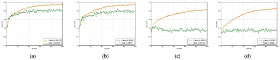
Figure 8.
Accuracy ratios of the classical DRSN with noise in this study. (a) Gaussian noise, (b) Poisson noise, (c) Speckle noise, and (d) Salt and Pepper noise.
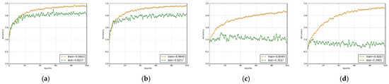
Figure 9.
Accuracy ratios of the Log-DRSN with noise in this study. (a) Gaussian noise, (b) Poisson noise, (c) Speckle noise, and (d) Salt and Pepper noise.
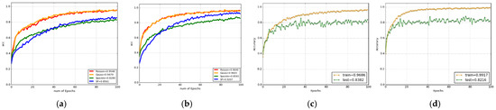
Figure 10.
Accuracy rates of the classical DRSN and Log-DRSN. (a) Classical DRSN from all noise, (b) Log-DRSN from all noise, (c) Classical DRSN without noise, and (d) Log-DRSN without noise.
Figure 11 illustrates the t-SNE visualizations of feature representations extracted by both the classical DRSN and the proposed Log-DRSN models. The clearer and more distinct clustering observed in the Log-DRSN visualization indicates its superior capability in learning discriminative features for fabric defect classification. When the accuracy rates of the models using both activation functions are examined in Table 3, it is clear that the Log-Leaky ReLU outperforms the traditional Leaky ReLU in terms of accuracy. Despite the increased computational complexity reflected in the computational times reported in Table 4, the Log-Leaky ReLU activation function, as implemented in the Log-DRSN model, was preferred in this study because achieving higher accuracy was prioritized over minimizing computation time.
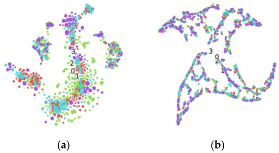
Figure 11.
t-SNE images obtained by executing the classical DRSN and the Log-DRSN. (a) Training samples and (b) samples with Log-DRSN.
Table 3.
Performance metrics of the classical DRSN and Log-DRSN.
Table 4.
Computational time of methods in this study.
When examining Figure 12, it is evident that Log-DRSN starts learning faster than the classical DRSN. This figure is based on the comparison of accuracy rates at three sample iteration points. In the fifth iteration, the classical DRSN reached 63%, while Log-DRSN achieved 87%. By the 15th iteration, the classical DRSN reached 83%, whereas Log-DRSN achieved an accuracy of 96%. In the 30th iteration, the classical DRSN reached 91%, and Log-DRSN achieved an impressive 98% accuracy. Similarly, Table 5 provides a more detailed comparison of learning rates. This table illustrates the accuracy rates of the two models between the 5th iteration and the 45th iteration. It becomes evident that Log-DRSN exhibits a faster learning pace compared to the classical model.
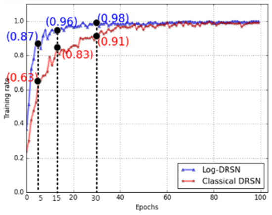
Figure 12.
Comparing the Log-DRSN and classical DRSN’ learning rates.
Table 5.
Learning rates in different iterations of the methods in this study.
4.3. Evaluation of Log-DRSN on Public Datasets
With the method proposed in our study, the classical DRSN method was also tested on public datasets such as MNIST, CIFAR-10, and Mini-ImageNet. As demonstrated by the experimental findings in Table 6, the Log-DRSN technique outperformed the regular DRSN in the literature, showing the highest accuracy on the Dataset_Fabric with 99.17% compared to 96.86%.
Table 6.
Comparison of classification accuracy between classical DRSN and Log-DRSN on multiple datasets.
4.4. Transfer Learning with Fine-Tuning on Our Dataset
Our dataset used in this study has been tested on different transfer learning models based on fine-tuning. The baseline models selected for comparison—InceptionV3, MobileNet, ResNet50, VGG16, and VGG19—were chosen due to their widespread use and proven performance in various image classification and defect detection tasks. These architectures represent a diverse set of design philosophies: from lightweight models (e.g., MobileNet) suitable for real-time applications to deeper and more complex networks (e.g., ResNet50, InceptionV3) that have demonstrated high accuracy in noise-prone environments. The results obtained were compared experimentally. Table 7 shows comparisons with transfer learning models such as InceptionV3, MobileNet, ResNet50, VGG16 and VGG19.
Table 7.
Transfer learning comparisons on our dataset.
To ensure a fair and consistent evaluation, all baseline models were adapted using transfer learning with fine-tuning strategies. Specifically, the pre-trained weights (initialized on ImageNet) were partially frozen to retain generic visual features, while the final layers were retrained on the fabric defect dataset to adapt to domain-specific patterns. The relatively modest performance of some models—such as ResNet50 and MobileNet—can be attributed to a combination of factors, including the domain gap between natural images in ImageNet and the fine-grained texture variations in fabric images. Additionally, these models may not be well-suited to capture the subtle, noise-prone, and small-scale defect patterns typical in fabric inspection. In particular, MobileNet’s lightweight architecture prioritizes computational efficiency over expressive capacity, which may lead to underfitting in complex defect detection tasks. On the other hand, models like VGG16 and VGG19, with deeper and more uniform convolutional structures, appear more capable of capturing the repetitive and localized nature of fabric defects, resulting in better precision and AUC values. This observation further validates the need for a specialized architecture, such as Log-DRSN, that integrates adaptive shrinkage and attention mechanisms tailored to noisy, domain-specific data.
4.5. Ablation Analysis of the Log-DRSN
Ablation analysis is used to determine which module is more important and effective for the performance of the proposed model. Log-DRSN has three basic modules. These are the residual shrinkage network (RSN) module, the attention (Attn.) module, and the soft thresholding (ST) module. In the proposed model, the RSN module consists of three blocks. For this reason, the units were gradually deactivated while examining the RSN module in ablation analysis. Although the contents of these units are similar, the number of filters is different, which changes the effectiveness of the units in the model. RSN unit-1, unit-2, and unit-3 filter numbers are 32, 64, and 128, respectively.
The Attention module, which creates a feature map, increases the model’s performance, and makes it more consistent. This module trains the model faster and more consistently. In addition, it accelerates model training and reduces the risk of overfitting. It contributes to obtaining better results as it ensures that the model is flexible and adaptive. The purpose of the soft thresholding module is to clean noisy data. It helps filter out unwanted noise, especially in data with a low signal-to-noise ratio. It contributes to increasing the model’s performance and plays an important role in training noisy image data. The RSN module is essential in training deep networks. This module not only simplifies the training process, but it also reduces overfitting. The network’s memory requirements are reduced when the Shrinkage module diminishes the size of the features that the network learns. Based on this data and Table 8, the outcomes that follow can be reached:
Table 8.
Performance metrics of different ablation studies.
- The attention module is the most essential component of the designed model because it extracts features. The factor that significantly impacted network performance was the removal of this module from the model. Similarly, it is the module that minimizes the model’s computation time most dramatically. The computation time was 365.0 s, and the accuracy rate was 26.48%. The removal of the attention module led to a dramatic 72–73% drop in accuracy compared to the baseline (over 96% range), underscoring its critical role in feature representation. The significant reduction in computation time (approximately 48% less than the full model’s ~705 s) also indicates this module’s computational cost, which is justified by its contribution to accuracy.
- When the first unit of the RSN module was omitted from the model, the accuracy of the model decreased slightly and the computation time slightly shortened as well. The computation time was 626.0 s, and the accuracy rate was 99.03%. The impact of removing RSN unit-1 was minimal, with an accuracy drop of only ~0.72%, suggesting that this unit contributes modestly to model robustness. The 11% decrease in computation time shows that this unit is somewhat costly computationally but not essential for peak accuracy.
- Once the second unit of the RSN module was eliminated from the model, the model’s accuracy rate declined more than RSN unit-1 and the calculation time was reduced even further. The calculation time was 605.0 s, and the accuracy rate was 98.29%. Removing RSN unit-2 caused a greater performance loss (1.46% drop) compared to unit-1, indicating a more important role in preserving discriminative features. However, its removal also resulted in a moderate 14% reduction in computation time, suggesting a balance between performance and efficiency.
- When the third unit of the RSN module was removed from the model, the accuracy rate of the model decreased the most when compared to the other two units. The calculation time has also been reduced the greatest with this choice. The accuracy rate was 96.40%, and the calculation time was 580.0 s. RSN unit-3 appears to be the most critical among the RSN components, with its removal resulting in a 2.6% accuracy reduction, the largest among RSN parts. At the same time, it yielded a 17.7% drop-in computation time, highlighting its computational load and its high influence on predictive power.
- The removal of the ST module from the model resulted in the least change in the model’s accuracy and complexity. The calculation time was 705.0 s, and the accuracy rate was 98.75. The negligible change in accuracy (<1%) and computation time indicates that the ST module has limited impact on overall model performance in this setup. This suggests that it may be optional or could be optimized further to justify its inclusion.
- When all alternatives are considered, the performance difference from greatest to smallest is Attention, RSN-3, RSN-2, RSN-1, and ST modules, in that order. This ranking aligns with quantitative findings, where the attention module alone accounts for the majority of accuracy loss (over 70%), while the RSN units show a graduated impact. The ST module’s limited effect confirms its position as the least critical component in terms of contribution to performance.
5. Conclusions
In this work, a novel deep learning-based model for classifying fabric faults is developed. We developed our own dataset to test the suggested concept empirically. The noise was manually added to the data to assess the noise resistance of the algorithms proposed in this study. The classical DRSN technique performed best with 96.86% accuracy and 765.0 s, DRSN based on the leaky activation performed best with 97.85% accuracy and 773.0 s, whereas the suggested Log-DRSN model performed best with 99.17% accuracy and 781.0 s. There is not much difference between the complexity times of the Leaky activation ReLU function and the Log-Leaky activation ReLU function, only a small amount of computation time due to the log operation is high in the log-leaky function. However, the accuracy rate of the log-leaky activation ReLU is higher than leaky activation, so the accuracy rate criterion is more critical for our study. It has been discovered that the proposed novel model is an effective strategy for both lowering computation time and providing good outcomes in terms of performance metrics.
However, it is important to acknowledge certain limitations and challenges associated with the proposed model. The experiments were conducted on a relatively small, custom dataset with synthetic noise, which may not fully represent the diversity of real-world fabric defects and environmental conditions. Moreover, the slightly increased computation time, while acceptable in offline or batch-processing contexts, could pose challenges for real-time inspection systems. It is also anticipated that utilizing higher computational resources—such as more powerful GPUs or parallel processing—would further improve both the training speed and overall performance of the model. Future work should focus on testing the model on larger, more diverse datasets and exploring optimization techniques to reduce inference time without compromising accuracy. Addressing these aspects will be essential for the successful deployment of the model in industrial fabric inspection settings.
Author Contributions
C.T.: conceptualization, investigation, design, analysis, writing—original draft; E.A.: data collection, analysis, writing—original draft and supervision; M.A.: writing and data collection. All authors have read and agreed to the published version of the manuscript.
Funding
This research received no external funding.
Institutional Review Board Statement
Not applicable.
Informed Consent Statement
Not applicable.
Data Availability Statement
The datasets generated and analyzed during the current study are not publicly available.
Acknowledgments
We would like to thank Agteks Ltd. for their valuable contributions to our dataset used in experimental studies.
Conflicts of Interest
Author Mehmet Agrikli was employed by the company Agteks. The remaining authors declare that the research was conducted in the absence of any commercial or financial relationships that could be construed as a potential conflict of interest.
References
- Hanbay, K.; Talu, M.F.; Özgüven, Ö.F.; Öztürk, D. Fabric defect detection methods for circular knitting machines. In Proceedings of the 2015 23rd Signal Processing and Communications Applications Conference (SIU), Malatya, Turkey, 16–19 May 2015; pp. 735–738. [Google Scholar] [CrossRef]
- Zhang, H.-W.; Zhang, L.-J.; Li, P.-F.; Gu, D. Yarn-dyed fabric defect detection with YOLOV2 based on deep convolution neural networks. In Proceedings of the 2018 IEEE 7th Data Driven Control and Learning Systems Conference (DDCLS), Enshi, China, 25–27 May 2018; pp. 170–174. [Google Scholar] [CrossRef]
- Wang, P.-H.; Lin, C.-C. Data augmentation method for fabric defect detection. In Proceedings of the 2022 IEEE International Conference on Consumer Electronics-Taiwan, Taipei, Taiwan, 6–8 July 2022; pp. 255–256. [Google Scholar] [CrossRef]
- Liu, K.-H.; Chen, S.-J.; Liu, T.-J. Unsupervised UNet for fabric defect detection. In Proceedings of the 2022 IEEE International Conference on Consumer Electronics-Taiwan, Taipei, Taiwan, 6–8 July 2022; pp. 205–206. [Google Scholar] [CrossRef]
- Liu, K.-H.; Chen, S.-J.; Chiu, C.-H.; Liu, T.-J. Fabric defect detection via unsupervised neural networks. In Proceedings of the 2022 IEEE International Conference on Multimedia and Expo Workshops (ICMEW), Taipei, Taiwan, 18–22 July 2022; pp. 1–6. [Google Scholar] [CrossRef]
- Lu, B.; Zhang, M.; Huang, B. Deep adversarial data augmentation for fabric defect classification with scarce defect data. IEEE Trans. Instrum. Meas. 2022, 71, 5014613. [Google Scholar] [CrossRef]
- Fang, B.; Long, X.; Sun, F.; Liu, H.; Zhang, S.; Fang, C. Tactile-Based fabric defect detection using convolutional neural network with attention mechanism. IEEE Trans. Instrum. Meas. 2022, 71, 5011309. [Google Scholar] [CrossRef]
- Shao, L.; Zhang, E.; Ma, Q.; Li, M. Pixel-Wise semisupervised fabric defect detection method combined with multitask mean teacher. IEEE Trans. Instrum. Meas. 2022, 71, 2506011. [Google Scholar] [CrossRef]
- Khodier, M.M.; Ahmed, S.M.; Sayed, M.S. Complex pattern jacquard fabrics defect detection using convolutional neural networks and multispectral imaging. IEEE Access 2022, 10, 10653–10660. [Google Scholar] [CrossRef]
- Liu, Q.; Wang, C.; Li, Y.; Gao, M.; Li, J. A fabric defect detection method based on deep learning. IEEE Access 2022, 10, 4284–4296. [Google Scholar] [CrossRef]
- Sudha, K.K.; Sujatha, P. Robust and rapid fabric defect detection using EGNet. In Proceedings of the 2021 4th International Conference on Computing and Communications Technologies (ICCCT), Chennai, India, 16–17 December 2021; pp. 494–499. [Google Scholar] [CrossRef]
- Xia, D.; Yu, Z.; Deng, X. A real-time unsupervised two-stage framework for fabric defect detection. In Proceedings of the 2021 3rd International Academic Exchange Conference on Science and Technology Innovation (IAECST), Guangzhou, China, 10–12 December 2021; pp. 535–538. [Google Scholar] [CrossRef]
- Zhang, Y.; Wu, Z.; Liu, Y.; Wang, C.; Yu, G. Fabric Defect Detection Based on Attention Mechanism and Improved YOLOv5 Network. IEEE Access 2023, 11, 12078–12089. [Google Scholar]
- Sakhare, K.; Kulkarni, A.; Kumbhakarn, M.; Kare, N. Spectral and spatial domain approach for fabric defect detection and classification. In Proceedings of the 2015 International Conference on Industrial Instrumentation and Control (ICIC), Pune, India, 28–30 May 2015; pp. 640–644. [Google Scholar] [CrossRef]
- Durmuşoğlu, A.; Kahraman, Y. Detection of fabric defects using convolutional networks. In Proceedings of the 2021 Innovations in Intelligent Systems and Applications Conference (ASYU), Elazig, Turkey, 6–8 October 2021; pp. 1–5. [Google Scholar] [CrossRef]
- Dafu, Y. Classification of fabric defects based on deep adaptive transfer learning. In Proceedings of the 2019 Chinese Automation Congress (CAC), Hangzhou, China, 22–24 November 2019; pp. 5730–5733. [Google Scholar] [CrossRef]
- Vladimir, G.; Evgen, I.; Aung, N.L. Automatic detection and classification of weaving fabric defects based on digital image processing. In Proceedings of the 2019 IEEE Conference of Russian Young Researchers in Electrical and Electronic Engineering (EIConRus), Saint Petersburg and Moscow, Russia, 28–31 January 2019; pp. 2218–2221. [Google Scholar] [CrossRef]
- Ma, Y.; Wang, C.; Jiang, C.; Li, Z. Deep residual shrinkage networks for EMG-based gesture identification. arXiv 2022, arXiv:2202.02984. [Google Scholar] [CrossRef]
- Zhao, M.; Zhong, S.; Fu, X.; Tang, B.; Pecht, M. Deep residual shrinkage networks for fault diagnosis. IEEE Trans. Ind. Inform. 2020, 16, 4681–4690. [Google Scholar] [CrossRef]
- Zhang, Z.; Li, H.; Chen, L. Deep residual shrinkage networks with self-adaptive slope thresholding for fault diagnosis. In Proceedings of the 2021 7th International Conference on Condition Monitoring of Machinery in Non-Stationary Operations (CMMNO), Guangzhou, China, 11–13 June 2021; pp. 236–239. [Google Scholar] [CrossRef]
- Paul, A. 4 Point System. Available online: https://www.scribd.com/doc/102427507/4-Point-System (accessed on 25 December 2022).
- Sarkar, P. How to Use 4 Point System in Fabric Inspection? Available online: https://www.onlineclothingstudy.com/2012/08/how-to-use-4-point-system-in-fabric.html (accessed on 25 December 2022).
- Zhou, Y.; Yuan, X.; Cui, X.; Song, Y.; Sun, Z.; Fan, J. Fault diagnosis based on deep residual shrinkage network and maximum mean discrepancy. In Proceedings of the 2021 China Automation Congress (CAC), Beijing, China, 22–24 October 2021; pp. 2340–2345. [Google Scholar] [CrossRef]
- Makandar, A.; Daneshwari, M.; Mahantesh, J. Comparative study of different noise models and effective filtering techniques. Int. J. Sci. Res. (IJSR) 2014, 3, 458–464. [Google Scholar]
- Boyat, A.K.; Joshi, B.K. A review paper: Noise models in digital image processing. arXiv 2015, arXiv:1505.03489. [Google Scholar] [CrossRef]
- Singh, P.; Shree, R. Speckle noise: Modelling and implementation. Int. J. Control. Theory Appl. 2016, 9, 8717–8727. [Google Scholar]
- Azzeh, J.; Zahran, B.; Alqadi, Z. Salt and pepper noise: Effects and removal. JOIV Int. J. Inform. Visual. 2018, 2, 252–256. [Google Scholar] [CrossRef]
- Bhatia, A. Salt and pepper noise removal from medical image through adaptive median filter. In Proceedings of the IT International Conference 2013, Washington, DC, USA, 16–17 November 2013. [Google Scholar]
- Liu, J.; Zhou, Q.; Zhang, B. Deep residual shrinkage network for few-shot learning. In Proceedings of the 2021 3rd International Conference on Intelligent Control, Measurement and Signal Processing and Intelligent Oil Field (ICMSP), Xi′an, China, 23–25 July 2021; pp. 120–124. [Google Scholar] [CrossRef]
- Cheng, L.; He, C. Fish recognition based on deep residual shrinkage network. In Proceedings of the 2021 4th International Conference on Robotics, Control and Automation Engineering (RCAE), Wuhan, China, 4–6 November 2021; pp. 36–39. [Google Scholar] [CrossRef]
- He, K.; Zhang, X.; Ren, S.; Sun, J. Delving deep into rectifiers: Surpassing human-level performance on imagenet classification. In Proceedings of the IEEE International Conference on Computer Vision, Santiago, Chile, 7–13 December 2015; pp. 1026–1034. [Google Scholar]
Disclaimer/Publisher’s Note: The statements, opinions and data contained in all publications are solely those of the individual author(s) and contributor(s) and not of MDPI and/or the editor(s). MDPI and/or the editor(s) disclaim responsibility for any injury to people or property resulting from any ideas, methods, instructions or products referred to in the content. |
© 2025 by the authors. Licensee MDPI, Basel, Switzerland. This article is an open access article distributed under the terms and conditions of the Creative Commons Attribution (CC BY) license (https://creativecommons.org/licenses/by/4.0/).