Dual-Dimensional Gaussian Splatting Integrating 2D and 3D Gaussians for Surface Reconstruction

Abstract

Three-Dimensional Gaussian Splatting (3DGS) has revolutionized novel-view synthesis, enabling real-time rendering of high-quality scenes. Two-Dimensional Gaussian Splatting (2DGS) improves geometric accuracy by replacing 3D Gaussians with flat 2D Gaussians. However, the flat nature of 2D Gaussians reduces mesh quality on volumetric surfaces and results in over-smoothed reconstruction. To address this, we propose Dual-Dimensional Gaussian Splatting (DDGS), which integrates both 2D and 3D Gaussians. First, we generalize the homogeneous transformation matrix based on 2DGS to initialize all Gaussians in 3D. Subsequently, during training, we selectively convert Gaussians into 2D representations based on their scale. This approach leverages the complementary strengths of 2D and 3D Gaussians, resulting in more accurate surface reconstruction across both flat and volumetric regions. Additionally, to mitigate over-smoothing, we introduce gradient-based regularization terms. Quantitative evaluations on the DTU and TnT datasets demonstrate that DDGS consistently outperforms prior methods, including 3DGS, SuGaR, and 2DGS, achieving the best Chamfer Distance and F1 score across a wide range of scenes.

1. Introduction

Novel view synthesis (NVS) and surface reconstruction from multi-view images are fundamental research fields in computer vision. These techniques aim to render photorealistic images from novel viewpoints or reconstruct accurate 3D meshes. They are essential for applications including 3D content creation [1,2], autonomous driving [3,4], virtual reality [5,6], and the metaverse [7,8].

Recently, Three-Dimensional Gaussian Splatting (3DGS) [9] has been proposed to represent a scene as a collection of 3D Gaussians, enabling efficient and high-quality real-time rendering. This is enabled by the differentiable nature of 3D Gaussians, along with efficient tile-based rasterization and optimization techniques. However, their volumetric nature makes it difficult to represent flat surfaces accurately, limiting their effectiveness in surface reconstruction. Moreover, affine transformations induced by each Gaussian’s covariance matrix can introduce geometric distortions that lead to projection errors.

Two-Dimensional Gaussian Splatting (2DGS) [10] replaces ellipsoid-shaped 3D Gaussians with oriented, elliptical disk-shaped 2D Gaussians, enhancing geometric detail in surface reconstruction. In addition, 2DGS replaces the covariance matrix with a homogeneous transformation matrix, allowing precise 2D-to-2D mapping. Depth maps are estimated to facilitate mesh extraction through truncated signed distance fusion (TSDF) using Open3D [11]. This depth information functions as a regularization term, encouraging the concentration of 2D Gaussians and aligning rendered normal vectors to achieve smoother surface reconstruction. However, these regularization constraints often lead to overly smooth surface reconstruction [10], further exacerbated by the limited capacity of 2D Gaussians to capture volumetric details.

In this paper, we introduce Dual-Dimensional Gaussian Splatting (DDGS), a novel hybrid representation that strategically integrates the complementary advantages of 2D and 3D Gaussians, to enhance flexibility and accuracy in surface reconstruction. Specifically, volumetric structures are modeled using 3D Gaussians, while flat surfaces are represented by 2D Gaussians, allowing adaptive selection of the optimal representation for different regions within a scene. This approach improves geometric accuracy across diverse environments by leveraging the complementary strengths of both representations.

Furthermore, we propose gradient-based regularization terms to improve mesh quality. Since the normal consistency term in 2DGS leads to excessively smoothed surfaces, we modulate it using a gradient-aware approach. This term aligns the rendered normal map with the normal map generated from the depth map. However, sharp depth changes can introduce errors, resulting in over-smoothed surfaces. To address this, we introduce a gradient-aware normal consistency term that applies stronger penalties in proportion to image gradients. Additionally, we incorporate regularization terms that minimize both the gradient and second-order gradient differences between the rendered and ground truth images, encouraging Gaussians to better fit the object surfaces.

In summary, the contributions of this paper are as follows:

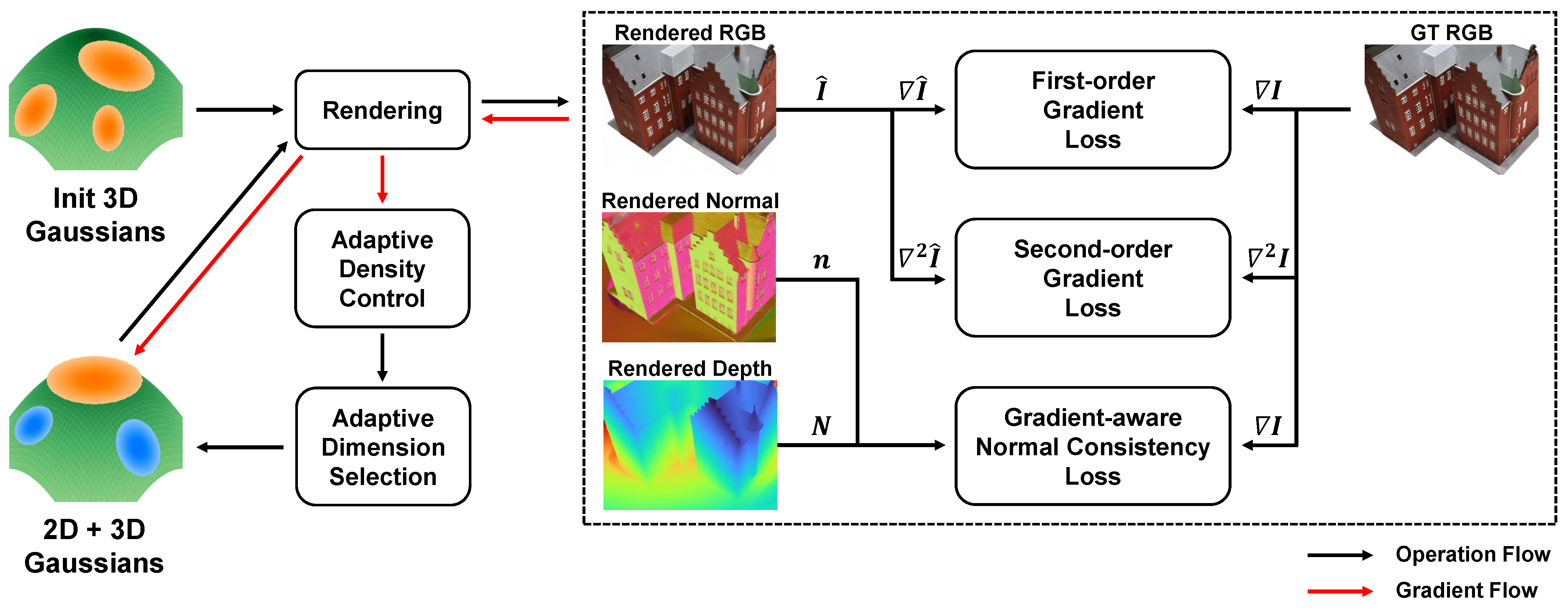
• We propose DDGS, which integrates both 2D and 3D Gaussians to enable flexible and precise surface reconstruction by adaptively selecting the optimal Gaussian representation based on the characteristics of the object surfaces.
• We introduce gradient-based regularization terms to improve the alignment accuracy between rendered Gaussian normals and the underlying ground truth surfaces, thus enhancing geometric fidelity.

2. Related Work

2.1. Novel View Synthesis with 3D Gaussians

Recently, 3D Gaussian Splatting (3DGS) [9] has demonstrated high-quality rendering at significantly higher speeds than prior implicit methods. By utilizing explicit and differentiable Gaussian representations, 3DGS accelerates both training and rendering without employing multi-layer perceptrons (MLPs). Additionally, each Gaussian employs spherical harmonics to efficiently render colors from all viewing directions. The real-time rendering capability of 3DGS has motivated extensive research on both performance optimization, such as accelerating training and rendering [12,13,14], and applications in various domains. In particular, 3DGS has been employed in simultaneous localization and mapping (SLAM) [15,16,17], interactive applications [18,19], and large-scale scene reconstruction [20,21]. Additionally, the integration of diffusion models has recently been explored to enhance 3D reconstruction performance across diverse environments [22,23]. Recent studies have further extended 3DGS to surface reconstruction tasks, aiming to enhance geometric accuracy and streamline mesh generation, thereby broadening its applicability in fields such as robotics [24], computer graphics [25], and augmented reality [26].

2.2. Surface Reconstruction with Gaussians

The Gaussians in 3DGS are distributed and do not align with object surfaces, making mesh generation challenging. SuGaR [25] introduced regularization terms that minimize both volume density differences and normal differences to better align Gaussians with object surfaces. SuGaR also employed Poisson reconstruction to obtain a triangle mesh. However, SuGaR involves computationally intensive regularization processes and often generates inaccurate meshes for planar surfaces due to difficulties in precisely aligning volumetric Gaussians to flat geometries. To address these issues, several studies have proposed regularization terms to flatten 3D Gaussians into 2D Gaussians [27,28]. Building on these approaches, 2D Gaussian Splatting (2DGS) [10] further develops this concept by reconstructing object surfaces with fully 2D Gaussians defined in the local tangent space. Furthermore, an exact homogeneous transformation for 2D Gaussians, along with regularization terms, facilitates efficient and accurate surface reconstruction.

2.3. Hybrid Representation with 2D and 3D Gaussians

Several recent methods have explored hybrid representations that combine 2D and 3D Gaussians. HybridGS [29] assigns 3D Gaussians to static regions to maintain view consistency, while employing 2D Gaussians for transient objects, enabling high-quality view synthesis under complex motion and occlusion. Mixed Gaussian Avatar [30] initially places 2D Gaussians on a facial mesh to ensure geometric alignment, and subsequently augments them with 3D Gaussians in areas where rendering quality is insufficient. MGSR [31] independently trains 2D and 3D Gaussians with mutual supervision. Specifically, 2D Gaussians assist lighting estimation in 3D, while 3D Gaussians guide surface reconstruction in 2D. This enhances photometric consistency and geometric accuracy under diverse lighting.

In contrast to these approaches, we focus on the flat and volumetric nature of 2D and 3D Gaussians to enhance surface reconstruction. Based on this perspective, we propose a hybrid approach, Dual-Dimensional Gaussian Splatting (DDGS), which integrates both 2D and 3D Gaussians to leverage their complementary strengths. To achieve this, we extend the homogeneous transformation to jointly handle both 2D and 3D Gaussians, and introduce an adaptive mechanism that selects the appropriate Gaussian dimensionality based on its scale. In addition, we employ gradient-based regularization terms to further enhance geometric accuracy.

3. Methods

3.1. Background

3D Gaussian Splatting (3DGS) [9] generates 3D Gaussians from a sparse point cloud to represent a scene. Each Gaussian is defined by its mean $\mathit{\mu }$, representing its position, and its covariance matrix $\mathrm{\Sigma }$, which encodes its shape and orientation in 3D space:

$$G\left(\mathbf{x}\right)=exp\left(-{\displaystyle \frac{1}{2}}{(\mathbf{x}-\mathit{\mu })}^T{\mathrm{\Sigma }}^{-1}(\mathbf{x}-\mathit{\mu })\right).$$

(1)

The covariance matrix is formulated using a scaling matrix $\mathbf{S}$ and a rotation matrix $\mathbf{R}$. The matrix $\mathbf{S}$ is parameterized by a 3D scaling vector, and $\mathbf{R}$ is represented using a 4D quaternion for rotation. However, to render the scene, the covariance matrix $\mathrm{\Sigma }$ in world space must be transformed into the covariance matrix ${\mathrm{\Sigma }}^{\prime }$ in camera coordinates. Given a viewing transformation $\mathbf{W}$ and a Jacobian $\mathbf{J}$ corresponding to the affine approximation of a projective transformation, the covariance matrix ${\mathrm{\Sigma }}^{\prime }$ is defined as follows:

$$\begin{array}{cc}\hfill \mathrm{\Sigma }& =\mathbf{R}\mathbf{S}{\mathbf{S}}^T{\mathbf{R}}^T,\hfill \\ \hfill {\mathrm{\Sigma }}^{\prime }& =\mathbf{J}\mathbf{W}\mathrm{\Sigma }{\mathbf{W}}^T{\mathbf{J}}^T.\hfill \end{array}$$

(2)

However, while the affine transformation accurately projects 3D Gaussians onto 2D Gaussians at their center, the approximation error accumulates as the distance from the center increases [10,32]. In particular, these errors can result in critical defects in surface reconstruction, such as holes in the reconstructed surface.

To address this issue, 2D Gaussian Splatting (2DGS) [10] incorporates a method based on homogeneous coordinate transformation. The $4\times 4$ homogeneous transformation matrix, encoding the scale and rotation information of the 2D Gaussians, is mapped to screen space by multiplying it by a $4\times 4$ world-to-screen transformation matrix. This precise 2D-to-2D mapping ensures the accurate projection of the Gaussians. However, representing curved surfaces with flat 2D Gaussians is challenging and often results in over-smoothed reconstructions.

3.2. Dual-Dimensional Gaussian Modeling

Figure 1 shows the overall flow of Dual-Dimensional Gaussian Splatting (DDGS), which combines 2D and 3D Gaussians. To implement this, we first augment the homogeneous transformation matrix with the w-axis to define the properties of a Gaussian in world space. A Gaussian is characterized by its learnable parameters, including its center $\mathit{\mu }$, tangent vectors ${\mathbf{t}}_u$, ${\mathbf{t}}_v$, ${\mathbf{t}}_w$, and scaling factors $s_u$, $s_v$, $s_w$. The tangent vectors are mutually orthogonal and form a $3\times 3$ rotation matrix $\mathbf{R}$, which represents the Gaussian’s orientation. Likewise, the scaling factors define the size and variance of the Gaussian and constitute the diagonal of a $3\times 3$ scaling matrix $\mathbf{S}$. The Gaussian is classified as a 3D Gaussian if all three scaling factors are nonzero, whereas it is considered a 2D Gaussian if exactly one of the scaling factors is zero. Finally, the homogeneous transformation matrix ${\mathbf{H}}^{*}$, which incorporates the additional w-axis compared to 2DGS, is defined as follows:

$${\mathbf{H}}^{*}=\left[\begin{array}{cccc}{s}_u{\mathbf{t}}_u& s_v{\mathbf{t}}_v& s_w{\mathbf{t}}_w& \mu \\ 0& 0& 0& 1\end{array}\right]=\left[\begin{array}{cc}\mathbf{RS}& \mathit{\mu }\\ 0& 1\end{array}\right].$$

(3)

This matrix enables the transformation of a Gaussian from local space to world space via ${\mathbf{H}}^{*}{(u,v,w,1)}^T$.

Figure 1. Overview of DDGS. The process begins with a set of 3D Gaussians. As training progresses, adaptive dimension selection based on scale transforms the representation into a hybrid of 2D and 3D Gaussians, where 2D Gaussians are assigned to flat regions and 3D Gaussians to complex surfaces.

Figure 1. Overview of DDGS. The process begins with a set of 3D Gaussians. As training progresses, adaptive dimension selection based on scale transforms the representation into a hybrid of 2D and 3D Gaussians, where 2D Gaussians are assigned to flat regions and 3D Gaussians to complex surfaces.

3.3. Adaptive Selection of 2D and 3D Gaussians

In our method, we classify a Gaussian as either 2D or 3D by determining whether one of its scaling factors should be set to zero. 3D Gaussians are well-suited for representing curved surfaces, whereas 2D Gaussians are more appropriate for flat surfaces. To fully leverage the strengths of both types, an appropriate dimensionality must be chosen for each Gaussian. To achieve this, we initialize all Gaussians as 3D and determine whether to convert them to 2D based on their scaling factors during training. Specifically, every 100 iterations, we evaluate the relative magnitudes of the scaling factors $s_u$, $s_v$, $s_w$. We empirically observe that if the smallest scaling factor is at least an order of magnitude smaller than the second smallest one, this factor is set to zero to enforce a 2D Gaussian representation. The robustness of this criterion is further analyzed in our experiments. For training stability, the transformation is applied only during the initial 40% of training, which coincides with the culling of low-opacity Gaussians and the progressive refinement of scene geometry. Following this phase, both the transformation and culling are discontinued, resulting in a stabilized structure.

With the exception of a single zero-valued scale factor, 2D and 3D Gaussians share the same learnable parameters and are processed identically during projection, blending, and rendering. To this end, we adopt a unified approach to the ray–Gaussian intersection.

3.4. Gaussian Splatting

To render a Gaussian, it is necessary to compute the intersection between the ray and the Gaussian in its local coordinate system. The Gaussian value at the intersection point $\mathbf{p}=(u,v,w)$ is computed as follows:

$$G=exp\left(-{\displaystyle \frac{{\parallel \mathbf{p}\parallel }^2}{2}}\right)=exp\left(-{\displaystyle \frac{u^2+v^2+w^2}{2}}\right).$$

(4)

In contrast to 2DGS, which uses only flat 2D Gaussians, our method employs both 2D and 3D Gaussians, necessitating more complex computations. To address this issue, we adopt the dual Plücker representation, following the approach of Hahlbohm et al. [33]. Given an image-space coordinate $(x,y)$, the corresponding ray can be represented as the intersection of two mutually orthogonal homogeneous planes, defined as the x-plane ${\mathbf{h}}_x={(-1,0,0,x)}^T$ and the y-plane ${\mathbf{h}}_y={(0,-1,0,y)}^T$. Given the world-to-screen transformation matrix $\mathbf{W}$, these planes are transformed into the Gaussian’s local space as follows:

$$\begin{array}{cc}\hfill {\mathbf{h}}_u& ={\left({\mathbf{WH}}^{*}\right)}^{-1}{\mathbf{h}}_x={\left({\mathbf{WH}}^{*}\right)}^T{\mathbf{h}}_x,\hfill \\ \hfill {\mathbf{h}}_v& ={\left({\mathbf{WH}}^{*}\right)}^{-1}{\mathbf{h}}_y={\left({\mathbf{WH}}^{*}\right)}^T{\mathbf{h}}_y.\hfill \end{array}$$

(5)

Here, ${\left({\mathbf{WH}}^{*}\right)}^T$ is equivalent to ${\left({\mathbf{WH}}^{*}\right)}^{-1}$ when applied to homogeneous planes [34].

The intersection of the two planes in the local space is expressed as a dual Plücker line ${\mathcal{L}}^{*}=(-\mathbf{m}:-\mathbf{d})$. In this representation, $\mathbf{d}$ represents the direction of the line, obtained as the cross product of the plane normals, while $\mathbf{m}$ is the moment vector derived from the plane normals and offsets. The two components of the line are computed as follows:

$$\begin{array}{cc}\hfill \mathbf{d}& =\left(h_u^0,h_u^1,h_u^2\right)\times \left(h_v^0,h_v^1,h_v^2\right),\hfill \\ \hfill \mathbf{m}& =h_u^3·\left(h_v^0,h_v^1,h_v^2\right)-h_v^3·\left(h_u^0,h_u^1,h_u^2\right).\hfill \end{array}$$

(6)

The intersection between the ray and the Gaussian in the local space is defined as the orthogonal projection of the Gaussian center onto the line ${\mathcal{L}}^{*}$ [33]. The projected point $\mathbf{p}$ is given by the following:

$$\mathbf{p}={\displaystyle \frac{\mathbf{d}\times \mathbf{m}}{{\parallel \mathbf{d}\parallel }^2}},{\parallel \mathbf{p}\parallel }^2={\displaystyle \frac{{\parallel \mathbf{d}\times \mathbf{m}\parallel }^2}{{\parallel \mathbf{d}\parallel }^4}}={\displaystyle \frac{{\parallel \mathbf{m}\parallel }^2}{{\parallel \mathbf{d}\parallel }^2}}.$$

(7)

The intersection point $\mathbf{p}$ enables both Gaussian value computation and depth retrieval via the homogeneous transform.

3.5. Optimization

We adopt the depth distortion and normal consistency losses from 2DGS, and incorporate new regularization terms into our method. In Gaussian splatting, when Gaussians at different depths contribute to the same pixel during blending, the estimated surface may deviate from the true geometry. The depth distortion loss encourages Gaussians to concentrate around the true surface, thereby reducing depth inconsistencies and improving geometric alignment.

$${\mathcal{L}}_d=\sum _{i,j}{\omega }_i{\omega }_j\left|z_i-z_j\right|$$

(8)

Here, ${\omega }_i$ and ${\omega }_j$ denote the blending weights at the i-th and j-th intersections, respectively, and $z_i$, $z_j$ represent their corresponding depths.

The normal consistency loss is effective in aligning Gaussians with the underlying surface geometry. It encourages the normal of each Gaussian to align with the surface normal estimated from the depth map gradient. However, estimating surface normals from nearby depth points can lead to errors in regions with high depth variation. These errors can result in excessive smoothing of the reconstructed surface. To address this issue, we introduce a gradient-aware normal consistency weight ${\omega }_{grad}$ to modulate the normal consistency loss:

$$\begin{array}{cc}\hfill {\mathcal{L}}_n^{*}=\sum _i{\omega }_i{\omega }_{grad}\left(1-{\mathbf{n}}_i^T\mathbf{N}\right),& \mathrm{where}{\omega }_{grad}=exp(-\parallel \nabla I\parallel ),\hfill \\ \hfill {\mathbf{n}}_i=\mathbf{R}·\mathrm{OneHot}& (argmin(s_u,s_v,s_w)).\hfill \end{array}$$

(9)

Here, ${\mathbf{n}}_i$ denotes the normal direction of the i-th Gaussian, computed by identifying the axis with the smallest scaling factor and applying the corresponding rotation, following the approach used in prior work [10,27,28]. In the case of 2D Gaussians, the normal direction is inherently determined by the axis associated with the zero-valued scaling factor. $\mathbf{N}$ is the surface normal estimated from the depth map, and $\nabla I$ represents the image gradient. ${\omega }_{grad}$ assigns lower weights to regions with strong image gradients, facilitating more accurate reconstruction of edge regions.

To enhance the representation of edge regions, we introduce both first-order and second-order gradient losses. The first-order loss penalizes image gradient differences, while the second-order loss captures curvature variations.

$$\begin{array}{cc}\hfill {\mathcal{L}}_{g1}& ={∥\nabla I-\nabla \widehat{I}∥}_1,\hfill \\ \hfill {\mathcal{L}}_{g2}& ={∥{\nabla }^{2}I-{\nabla }^2\widehat{I}∥}_1\hfill \end{array}$$

(10)

Here, I and $\widehat{I}$ denote the ground-truth and predicted images, respectively. These losses optimize learnable Gaussian parameters, leading to improved reconstruction of both edges and curvature, and better alignment with underlying surfaces.

Finally, we optimize the following loss function:

$$\mathcal{L}={\mathcal{L}}_c+{\lambda }_d{\mathcal{L}}_d+{\lambda }_n{\mathcal{L}}_n^{*}+{\lambda }_{g1}{\mathcal{L}}_{g1}+{\lambda }_{g2}{\mathcal{L}}_{g2}.$$

(11)

Here, ${\mathcal{L}}_c$ is the appearance loss defined in 3DGS, consisting of a weighted sum of the PSNR and SSIM losses, with weights of 0.8 and 0.2, respectively.

4. Experiments and Discussion

4.1. Implementation Details

We increase the number of Gaussians through adaptive densification, following the 3DGS strategy, until reaching 15,000 iterations out of the total 30,000 iterations. During the first 12,000 iterations, we determine the dimensionality of each Gaussian every 100 iterations by adaptively selecting between 2D and 3D Gaussians. For the proposed gradient-based regularization terms, we compute image gradients from both the ground-truth and rendered images at every iteration. The rasterization process follows the 2DGS approach and is performed at every iteration via volumetric alpha blending.

We compare DDGS with existing explicit methods, including 3DGS [9], SuGaR [25], and 2DGS [10]. To comprehensively evaluate our method, we assess its performance on three datasets across different environments. For surface reconstruction evaluation, we use the DTU dataset [35], which contains multi-view scans of small objects, and the Tanks and Temples (TnT) dataset [36], which provides large-scale 360-degree scenes. For image rendering quality, we use the Mip-NeRF 360 dataset [37], which includes a variety of indoor and outdoor environments. The indoor scenes in Mip-NeRF 360 include bonsai, counter, kitchen, and room, while the outdoor scenes consist of bicycle, flowers, garden, stump, and treehill. We evaluate surface reconstruction using Chamfer Distance and F1 score, and 2D image appearance quality with PSNR, SSIM, and LPIPS.

Chamfer Distance measures the average closest-point distance between the reconstructed and ground-truth surfaces.

$$\mathrm{CD}(P,G)={\displaystyle \frac{1}{2}}\left({\displaystyle \frac{1}{\left|P\right|}}\sum _{p\in P}\underset{g\in G}{min}{\parallel p-g\parallel }^2+{\displaystyle \frac{1}{\left|G\right|}}\sum _{g\in G}\underset{p\in P}{min}{\parallel g-p\parallel }^2\right)$$

(12)

Here, P is the predicted point set sampled from the reconstructed mesh, and G is the ground truth point set.

The F1 score is the harmonic mean of precision and recall for the reconstructed surfaces. Both metrics are computed using a distance threshold d between predicted and ground truth points.

$$\begin{array}{cc}\hfill \mathrm{Precision}\left(d\right)& ={\displaystyle \frac{\left|\right\{p\in P:{min}_{g\in G}\parallel p-g\parallel <d\left\}\right|}{\left|P\right|}},\hfill \\ \hfill \mathrm{Recall}\left(d\right)& ={\displaystyle \frac{\left|\right\{g\in G:{min}_{p\in P}\parallel g-p\parallel <d\left\}\right|}{\left|G\right|}},\hfill \\ \hfill \text{F1-score}\left(d\right)& ={\displaystyle \frac{2·\mathrm{Precision}\left(d\right)·\mathrm{Recall}\left(d\right)}{\mathrm{Precision}\left(d\right)+\mathrm{Recall}\left(d\right)}}\hfill \end{array}$$

(13)

The Peak Signal-to-Noise Ratio (PSNR) quantifies image similarity based on pixel-wise mean squared error.

$$\mathrm{PSNR}=10·{log}_{10}\left({\displaystyle \frac{{\mathrm{MAX}}_I^2}{\mathrm{MSE}}}\right)$$

(14)

Here, ${\mathrm{MAX}}_I$ denotes the maximum pixel intensity value, and $\mathrm{MSE}$ represents the mean squared error between the predicted and ground truth images.

The Structural Similarity Index (SSIM) compares images based on luminance, contrast, and structural similarity.

$$\mathrm{SSIM}(x,y)={\displaystyle \frac{(2{\mu }_x{\mu }_y+C_1)(2{\sigma }_{xy}+C_2)}{({\mu }_x^2+{\mu }_y^2+C_1)({\sigma }_x^2+{\sigma }_y^2+C_2)}}$$

(15)

Here, ${\mu }_x$ and ${\mu }_y$ are local means, ${\sigma }_x^2$ and ${\sigma }_y^2$ are variances, and ${\sigma }_{xy}$ is the covariance between images x and y. $C_1$ and $C_2$ are small constants for numerical stability.

The Learned Perceptual Image Patch Similarity (LPIPS) measures perceptual similarity using deep features from neural networks.

$$\mathrm{LPIPS}(x,x_0)=\sum _l{\displaystyle \frac{1}{H_l{W}_l}}\sum _{h,w}{∥w_l\odot \left({\widehat{y}}_{hw}^l-{\widehat{y}}_{0hw}^l\right)∥}_2^2$$

(16)

Here, ${\widehat{y}}_{hw}^l$ and ${\widehat{y}}_{0hw}^l$ are the normalized deep features at spatial location $(h,w)$ from layer l for images x and $x_0$, respectively, and $w_l$ denotes learned channel-wise weights. $H_l$ and $W_l$ are the spatial dimensions of layer l.

Following 2DGS, we set ${\lambda }_d$ to 1000 for unbounded scenes, 100 for bounded 360-degree scenes, and 0 for large-scale scenes such as Mip-NeRF 360. Similarly, ${\lambda }_n$ is fixed to 0.05 across all environments. The weights for our gradient losses are set to ${\lambda }_{g1}=0.3$ and ${\lambda }_{g2}=0.7$ by default. The weights are reduced to 0.1 for large-scale scenes, specifically the outdoor scenes in the Mip-NeRF 360 dataset and the Courthouse and Meetingroom scenes in the TnT dataset. For mesh extraction, we use a voxel size of 0.004 and a truncation threshold of 0.02, following the same setting as 2DGS. We conduct all experiments on a single RTX 3090 GPU at 1/2 resolution, except for the large-scale outdoor scenes in Mip-NeRF 360, which are evaluated at 1/4 resolution.

4.2. Evaluation and Analysis

In

Table 1. Quantitative comparison of Chamfer Distance (mm) and training time on the DTU dataset [35]. Lower Chamfer Distance ↓ and training time ↓ indicate better performance. Bold indicates the best performance, and italic indicates the second-best.

Methods	DTU Scene ID															Mean
	24	37	40	55	63	65	69	83	97	105	106	110	114	118	122	CD↓	Time↓
3DGS	2.54	1.35	2.03	1.77	3.07	2.61	1.79	2.20	2.15	1.87	2.05	2.38	1.89	1.65	1.72	2.07	6 min
SuGaR	1.79	1.05	1.04	0.69	1.86	1.59	1.27	1.80	1.86	1.31	1.01	1.83	1.37	1.04	0.83	1.36	39 min
2DGS	0.50	0.81	0.34	0.43	0.94	0.85	0.82	1.28	1.21	0.64	0.69	1.37	0.42	0.67	0.48	0.76	11 min
Ours	0.47	0.81	0.34	0.41	0.91	0.84	0.76	1.20	1.10	0.63	0.65	1.10	0.40	0.57	0.42	0.71	15 min

, we compare the Chamfer Distance and training time for the DTU dataset. Among all compared methods, our method DDGS achieves the lowest average Chamfer Distance, indicating the highest reconstruction accuracy overall. In particular, DDGS significantly improves surface reconstruction quality over the base model, 2DGS, across all scenes in the DTU dataset. This improvement, however, comes with a slight increase in average training time. Figure 2 shows the spatial distribution of 2D and 3D Gaussians, reflecting DDGS’s adaptive assignment based on surface geometry.

Table 2. Quantitative comparison of F1 score and training time on the Tanks and Temples dataset [36]. Higher F1 score ↑ and lower training time ↓ indicate better performance. Bold indicates the best performance, and italic indicates the second-best.

Methods	TnT Scene ID						Mean
	Barn	Caterpillar	Courthouse	Ignatius	Meetingroom	Truck	F1-Score↑	Time↓
3DGS	0.16	0.13	0.08	0.20	0.12	0.21	0.15	14 min
SuGaR	0.06	0.07	0.03	0.17	0.09	0.21	0.11	50 min
2DGS	0.39	0.24	0.16	0.50	0.20	0.45	0.32	16 min
Ours	0.38	0.23	0.16	0.51	0.20	0.54	0.34	23 min

compares the F1 score and training time on the TnT dataset. DDGS achieves the highest average F1 score among all methods and demonstrates particularly high accuracy on the Truck scene. Similar to the DTU results, DDGS consistently requires more training time than 2DGS. Figure 3 shows qualitative improvements in surface reconstruction quality with DDGS.

Table 3. Quantitative comparison on the Mip-NeRF 360 dataset [37]. Higher PSNR ↑ and SSIM ↑, and lower LPIPS ↓ and training time ↓ indicate better performance. Bold indicates the best performance, and italic indicates the second-best.

Methods	Outdoor Scene (Mean)				Indoor Scene (Mean)
	PSNR ↑	SSIM ↑	LPIPS ↓	Time ↓	PSNR ↑	SSIM ↑	LPIPS ↓	Time ↓
3DGS	24.60	0.726	0.240	29 min	30.91	0.923	0.188	23 min
SuGaR	22.94	0.647	0.312	66 min	29.46	0.906	0.208	58 min
2DGS	24.16	0.702	0.288	33 min	30.03	0.909	0.214	35 min
Ours	24.24	0.713	0.267	40 min	29.44	0.908	0.205	46 min

presents a comparison of PSNR, SSIM, LPIPS, and training time on the Mip-NeRF 360 dataset, which does not provide surface ground truth. Although DDGS enhances surface quality, its rendering performance is lower than that of 3DGS. This trade-off is expected because our method is specifically designed to enhance surface reconstruction and mesh extraction, where mesh-quality metrics such as Chamfer Distance and F1 score are more relevant than image-quality metrics used in image rendering, such as PSNR, SSIM, and LPIPS. While DDGS sacrifices some rendering fidelity, it significantly improves geometric accuracy, which is the primary goal of this work. Nevertheless, DDGS maintains rendering performance comparable to 2DGS, indicating a substantial improvement in geometry while preserving reasonable visual quality. Figure 4 shows qualitative improvements in surface reconstruction.

This enhancement in surface reconstruction can be attributed to DDGS’s adaptive assignment of Gaussian dimensionality based on local surface geometry. Specifically, DDGS assigns 2D Gaussians to flat surfaces and 3D Gaussians to geometrically complex or volumetric regions. This adaptive strategy enables more effective modeling of diverse surface structures within a scene. As shown in Figure 2, 3DGS captures geometrically complex surfaces relatively well but fails to accurately reconstruct large, flat regions. In contrast, 2DGS effectively models flat surfaces but tends to over-smooth complex structures. DDGS instead adaptively selects between 2D and 3D Gaussians based on local geometry, resulting in more detailed and accurate surface reconstruction across varying surface types.

Moreover, we conduct quantitative analyses to evaluate the effectiveness of the proposed regularization terms. The evaluation is based on the average Chamfer Distance computed over 15 scenes from the DTU dataset. In

Table 4. Quantitative comparison of Chamfer Distance (mm) for the ablation study of the regularization terms on the DTU dataset [35]. We report the average Chamfer Distance across 15 scenes. Lower Chamfer Distance ↓ indicates better performance. Bold indicates the best performance, and italic indicates the second-best.

Ablation Setting	${\mathit{\omega }}_{\mathbf{grad}}$	${\mathit{\lambda }}_{\mathit{g}1}$	${\mathit{\lambda }}_{\mathit{g}2}$	Mean CD ↓
w/o gradient-aware normal consistency weight		✓	✓	0.7239
w/o first-order gradient loss	✓		✓	0.7216
w/o second-order gradient loss	✓	✓		0.7457
Full model	✓	✓	✓	0.7074

, we compare our full model, which incorporates all regularization terms, with ablated versions where each term is removed individually. Removing any of the regularization terms—including the gradient-aware normal consistency weight ${\omega }_{grad}$, the first-order gradient loss ${\lambda }_{g1}$, or the second-order gradient loss ${\lambda }_{g2}$—consistently results in degraded surface reconstruction quality. Among these, removing ${\lambda }_{g2}$ leads to the largest performance drop, indicating the importance of curvature-level alignment. These results demonstrate the complementary contributions of each regularization term in our design.

We empirically found that when the smallest scaling factor is more than ten times smaller than the second smallest one, the Gaussian should be transformed into a 2D representation. To validate the robustness of this threshold, we conducted an ablation study by varying the ratio from 5 to 30, as shown in

Table 5. Quantitative comparison of Chamfer Distance (mm) for the ablation study on the ratio threshold for transforming 3D Gaussians into 2D on the DTU dataset [35]. We report the average Chamfer Distance across 15 scenes. Lower Chamfer Distance ↓ indicates better performance. Bold indicates the best performance, and italic indicates the second-best.

Ratio Threshold	5	10	15	20	25	30
Mean Chamfer Distance ↓	0.7248	0.7074	0.7159	0.7170	0.7144	0.7123

. Using Chamfer Distance on the DTU dataset as the evaluation metric, we observed the best performance at a ratio threshold of 10, with only negligible variations up to 30. These results indicate that the threshold criterion is not overly sensitive and remains sufficiently robust.

We evaluate both image rendering speed and mean mesh extraction time for each dataset, as summarized in

Table 6. Quantitative comparison of image rendering speed and mesh extraction time on the DTU [35], Tanks and Temples [36], and Mip-NeRF 360 [37] datasets. Higher speed ↑ and lower time ↓ indicate better performance. Bold indicates the best performance, and italic indicates the second-best.

Method	Image Rendering Speed ↑ (fps)			Mean Mesh Extraction Time ↓ (s)
	DTU	TnT	Mip-NeRF 360	DTU	TnT	Mip-NeRF 360
3DGS	261.27	163.14	97.55	1.36	376.24	58.59
SuGaR	78.74	82.02	72.79	98.11	295.15	471.96
2DGS	140.30	112.33	50.29	1.52	158.60	42.70
Ours	102.91	82.43	43.92	1.49	178.62	43.15

. Image rendering speed is generally proportional to training speed. Although our method is slower than both 3DGS and 2DGS, it still achieves real-time rendering performance. Furthermore, similar to training speed, all methods except for SuGaR are sensitive to scene scale.

DDGS shows mesh extraction efficiency comparable to 2DGS and 3DGS due to their common use of a TSDF-based reconstruction pipeline. While mesh extraction follows similar trends to image rendering, it is considerably more sensitive to scene scale, particularly in large-scale scenes within the TnT dataset. In contrast, SuGaR, which employs Poisson surface reconstruction, generally requires more time for mesh extraction.

5. Conclusions

In this paper, we introduced DDGS, a hybrid approach for accurate surface reconstruction that leverages both 2D and 3D Gaussians. By combining the strengths of 2D and 3D representations, DDGS adapts the Gaussian dimensionality based on spatial scale, enabling more flexible and precise modeling of complex surfaces. We further proposed gradient-based regularization terms to mitigate over-smoothing and enhance surface alignment. DDGS achieves superior surface reconstruction accuracy across both flat and volumetric regions, as demonstrated by experimental results on the DTU and TnT datasets, where it outperforms prior methods such as 3DGS, SuGaR, and 2DGS in terms of Chamfer Distance and F1 score. Nevertheless, DDGS still struggles to accurately reconstruct challenging regions such as semi-transparent surfaces and specular highlights, often resulting in incomplete geometry or visible holes in the reconstructed mesh. This limitation mainly stems from the difficulty of Gaussian Splatting in modeling high-frequency, view-dependent reflections. Addressing these issues remains an important direction for future work, potentially through the integration of shading functions to better capture reflective effects.

References

1. Tang, J.; Ren, J.; Zhou, H.; Liu, Z.; Zeng, G. Dreamgaussian: Generative gaussian splatting for efficient 3D content creation. arXiv 2023, arXiv:2309.16653. [Google Scholar]
2. Tang, J.; Chen, Z.; Chen, X.; Wang, T.; Zeng, G.; Liu, Z. Lgm: Large multi-view gaussian model for high-resolution 3D content creation. In Proceedings of the European Conference on Computer Vision, Milan, Italy, 29 September 29–4 October 2024; pp. 1–18. [Google Scholar]
3. Tonderski, A.; Lindström, C.; Hess, G.; Ljungbergh, W.; Svensson, L.; Petersson, C. Neurad: Neural rendering for autonomous driving. In Proceedings of the IEEE/CVF Conference on Computer Vision and Pattern Recognition, Seattle, WA, USA, 16–22 June 2024; pp. 14895–14904. [Google Scholar]
4. Wang, J.; Zhu, X.; Chen, Z.; Li, P.; Jiang, C.; Zhang, H.; Yu, C.; Yu, B. SRNeRF: Super-Resolution Neural Radiance Fields for Autonomous Driving Scenario Reconstruction from Sparse Views. World Electr. Veh. J. 2025, 16, 66. [Google Scholar] [CrossRef]
5. Deng, N.; He, Z.; Ye, J.; Duinkharjav, B.; Chakravarthula, P.; Yang, X.; Sun, Q. Fov-nerf: Foveated neural radiance fields for virtual reality. IEEE Trans. Vis. Comput. Graph. 2022, 28, 3854–3864. [Google Scholar] [CrossRef] [PubMed]
6. Lian, H.; Liu, K.; Cao, R.; Fei, Z.; Wen, X.; Chen, L. Integration of 3D Gaussian Splatting and Neural Radiance Fields in Virtual Reality Fire Fighting. Remote Sens. 2024, 16, 2448. [Google Scholar] [CrossRef]
7. Abramov, N.; Lankegowda, H.; Liu, S.; Barazzetti, L.; Beltracchi, C.; Ruttico, P. Implementing Immersive Worlds for Metaverse-Based Participatory Design through Photogrammetry and Blockchain. ISPRS Int. J. Geo-Inf. 2024, 13, 211. [Google Scholar] [CrossRef]
8. Fabra, L.; Solanes, J.E.; Muñoz, A.; Martí-Testón, A.; Alabau, A.; Gracia, L. Application of Neural Radiance Fields (NeRFs) for 3D model representation in the industrial metaverse. Appl. Sci. 2024, 14, 1825. [Google Scholar] [CrossRef]
9. Kerbl, B.; Kopanas, G.; Leimkühler, T.; Drettakis, G. 3D gaussian splatting for real-time radiance field rendering. ACM Trans. Graph. 2023, 42, 139. [Google Scholar] [CrossRef]
10. Huang, B.; Yu, Z.; Chen, A.; Geiger, A.; Gao, S. 2d gaussian splatting for geometrically accurate radiance fields. In Proceedings of the ACM SIGGRAPH 2024 Conference Papers, Denver, CO, USA, 27 July–1 August 2024; pp. 1–11. [Google Scholar]
11. Zhou, Q.Y.; Park, J.; Koltun, V. Open3D: A modern library for 3D data processing. arXiv 2018, arXiv:1801.09847. [Google Scholar]
12. Lu, T.; Yu, M.; Xu, L.; Xiangli, Y.; Wang, L.; Lin, D.; Dai, B. Scaffold-gs: Structured 3D gaussians for view-adaptive rendering. In Proceedings of the IEEE/CVF Conference on Computer Vision and Pattern Recognition, Seattle, WA, USA, 16–22 June 2024; pp. 20654–20664. [Google Scholar]
13. Fan, Z.; Wang, K.; Wen, K.; Zhu, Z.; Xu, D.; Wang, Z. Lightgaussian: Unbounded 3D gaussian compression with 15x reduction and 200+ fps. Adv. Neural Inf. Process. Syst. 2024, 37, 140138–140158. [Google Scholar]
14. Qiu, S.; Wu, C.; Wan, Z.; Tong, S. High-Fold 3D Gaussian Splatting Model Pruning Method Assisted by Opacity. Appl. Sci. 2025, 15, 1535. [Google Scholar] [CrossRef]
15. Guo, C.; Gao, C.; Bai, Y.; Lv, X. RD-SLAM: Real-Time Dense SLAM Using Gaussian Splatting. Appl. Sci. 2024, 14, 7767. [Google Scholar] [CrossRef]
16. Zhu, F.; Zhao, Y.; Chen, Z.; Jiang, C.; Zhu, H.; Hu, X. DyGS-SLAM: Realistic Map Reconstruction in Dynamic Scenes Based on Double-Constrained Visual SLAM. Remote Sens. 2025, 17, 625. [Google Scholar] [CrossRef]
17. Ma, X.; Song, C.; Ji, Y.; Zhong, S. Related Keyframe Optimization Gaussian–Simultaneous Localization and Mapping: A 3D Gaussian Splatting-Based Simultaneous Localization and Mapping with Related Keyframe Optimization. Appl. Sci. 2025, 15, 1320. [Google Scholar] [CrossRef]
18. Choi, S.; Song, H.; Kim, J.; Kim, T.; Do, H. Click-gaussian: Interactive segmentation to any 3D gaussians. In Proceedings of the European Conference on Computer Vision, Milan, Italy, 29 September–4 October 2024; pp. 289–305. [Google Scholar]
19. Dong, S.; Ding, L.; Huang, Z.; Wang, Z.; Xue, T.; Xu, D. Interactive3d: Create what you want by interactive 3D generation. In Proceedings of the IEEE/CVF Conference on Computer Vision and Pattern Recognition, Seattle, WA, USA, 16–22 June 2024; pp. 4999–5008. [Google Scholar]
20. Liu, Y.; Luo, C.; Fan, L.; Wang, N.; Peng, J.; Zhang, Z. Citygaussian: Real-time high-quality large-scale scene rendering with gaussians. In Proceedings of the European Conference on Computer Vision, Milan, Italy, 29 September–4 October 2024; pp. 265–282. [Google Scholar]
21. Shaheen, B.; Zane, M.D.; Bui, B.T.; Shubham; Huang, T.; Merello, M.; Scheelk, B.; Crooks, S.; Wu, M. ForestSplat: Proof-of-Concept for a Scalable and High-Fidelity Forestry Mapping Tool Using 3D Gaussian Splatting. Remote Sens. 2025, 17, 993. [Google Scholar] [CrossRef]
22. Mu, Y.; Zuo, X.; Guo, C.; Wang, Y.; Lu, J.; Wu, X.; Xu, S.; Dai, P.; Yan, Y.; Cheng, L. Gsd: View-guided gaussian splatting diffusion for 3D reconstruction. In Proceedings of the European Conference on Computer Vision, Milan, Italy, 29 September–4 October 2024; pp. 55–72. [Google Scholar]
23. Mithun, N.C.; Pham, T.; Wang, Q.; Southall, B.; Minhas, K.; Matei, B.; Mandt, S.; Samarasekera, S.; Kumar, R. Diffusion-Guided Gaussian Splatting for Large-Scale Unconstrained 3D Reconstruction and Novel View Synthesis. arXiv 2025, arXiv:2504.01960. [Google Scholar]
24. Lou, H.; Liu, Y.; Pan, Y.; Geng, Y.; Chen, J.; Ma, W.; Li, C.; Wang, L.; Feng, H.; Shi, L.; et al. Robo-gs: A physics consistent spatial-temporal model for robotic arm with hybrid representation. arXiv 2024, arXiv:2408.14873. [Google Scholar]
25. Guédon, A.; Lepetit, V. Sugar: Surface-aligned gaussian splatting for efficient 3D mesh reconstruction and high-quality mesh rendering. In Proceedings of the IEEE/CVF Conference on Computer Vision and Pattern Recognition, Seattle, WA, USA, 16–22 June 2024; pp. 5354–5363. [Google Scholar]
26. Zhai, H.; Zhang, X.; Zhao, B.; Li, H.; He, Y.; Cui, Z.; Bao, H.; Zhang, G. Splatloc: 3D gaussian splatting-based visual localization for augmented reality. IEEE Trans. Vis. Comput. Graph. 2025, 31, 3591–3601. [Google Scholar] [CrossRef]
27. Chen, H.; Li, C.; Lee, G.H. Neusg: Neural implicit surface reconstruction with 3D gaussian splatting guidance. arXiv 2023, arXiv:2312.00846. [Google Scholar]
28. Turkulainen, M.; Ren, X.; Melekhov, I.; Seiskari, O.; Rahtu, E.; Kannala, J. Dn-splatter: Depth and normal priors for gaussian splatting and meshing. arXiv 2024, arXiv:2403.17822. [Google Scholar]
29. Lin, J.; Gu, J.; Fan, L.; Wu, B.; Lou, Y.; Chen, R.; Liu, L.; Ye, J. HybridGS: Decoupling Transients and Statics with 2D and 3D Gaussian Splatting. arXiv 2024, arXiv:2412.03844. [Google Scholar]
30. Chen, P.; Wei, X.; Wuwu, Q.; Wang, X.; Xiao, X.; Lu, M. MixedGaussianAvatar: Realistically and Geometrically Accurate Head Avatar via Mixed 2D-3D Gaussian Splatting. arXiv 2024, arXiv:2412.04955. [Google Scholar]
31. Zhou, Q.; Gong, Y.; Yang, W.; Li, J.; Luo, Y.; Xu, B.; Li, S.; Fei, B.; He, Y. MGSR: 2D/3D Mutual-boosted Gaussian Splatting for High-fidelity Surface Reconstruction under Various Light Conditions. arXiv 2025, arXiv:2503.05182. [Google Scholar]
32. Zwicker, M.; Rasanen, J.; Botsch, M.; Dachsbacher, C.; Pauly, M. Perspective accurate splatting. In Proceedings of the Graphics Interface, London, ON, Canada, 17–19 May 2004; pp. 247–254. [Google Scholar]
33. Hahlbohm, F.; Friederichs, F.; Weyrich, T.; Franke, L.; Kappel, M.; Castillo, S.; Stamminger, M.; Eisemann, M.; Magnor, M. Efficient Perspective-Correct 3D Gaussian Splatting Using Hybrid Transparency. arXiv 2024, arXiv:2410.08129. [Google Scholar] [CrossRef]
34. Blinn, J.F. A homogeneous formulation for lines in 3 space. In Proceedings of the 4th Annual Conference on Computer Graphics and Interactive Techniques, San Jose, CA, USA, 20–22 July 1977; pp. 237–241. [Google Scholar]
35. Jensen, R.; Dahl, A.; Vogiatzis, G.; Tola, E.; Aanæs, H. Large scale multi-view stereopsis evaluation. In Proceedings of the IEEE Conference on Computer Vision and Pattern Recognition, Columbus, OH, USA, 23–28 June 2014; pp. 406–413. [Google Scholar]
36. Knapitsch, A.; Park, J.; Zhou, Q.Y.; Koltun, V. Tanks and temples: Benchmarking large-scale scene reconstruction. ACM Trans. Graph. 2017, 36, 1–13. [Google Scholar] [CrossRef]
37. Barron, J.T.; Mildenhall, B.; Verbin, D.; Srinivasan, P.P.; Hedman, P. Mip-nerf 360: Unbounded anti-aliased neural radiance fields. In Proceedings of the IEEE/CVF Conference on Computer Vision and Pattern Recognition, New Orleans, LA, USA, 18–24 June 2022; pp. 5470–5479. [Google Scholar]
Figure 2. Qualitative comparison on the DTU dataset [35]. The first row visualizes the distribution of 2D and 3D Gaussians: 3D Gaussians are shown in orange, and 2D Gaussians in blue. For DDGS, 2D Gaussians are primarily used on flat surfaces, while 3D Gaussians are applied to complex volumetric structures. The second and third rows show surface reconstruction results across different methods.
Applsci 15 06769 g002
Figure 3. Qualitative comparison on the Tanks and Temples dataset [36]. DDGS demonstrates more precise and detailed surface reconstruction than other methods.
Applsci 15 06769 g003
Figure 4. Qualitative comparison on the Mip-NeRF 360 dataset [37]. Compared to other methods, DDGS achieves more accurate and detailed surface reconstruction.
Applsci 15 06769 g004