
Prediction and Parameter Optimization of Surface Settlement Induced by Shield Tunneling Using Improved Informer Algorithm


Abstract
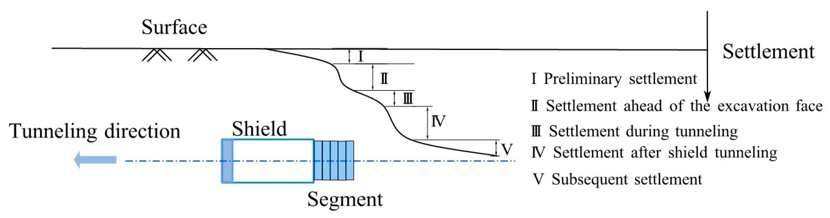
1. Introduction
2. Method
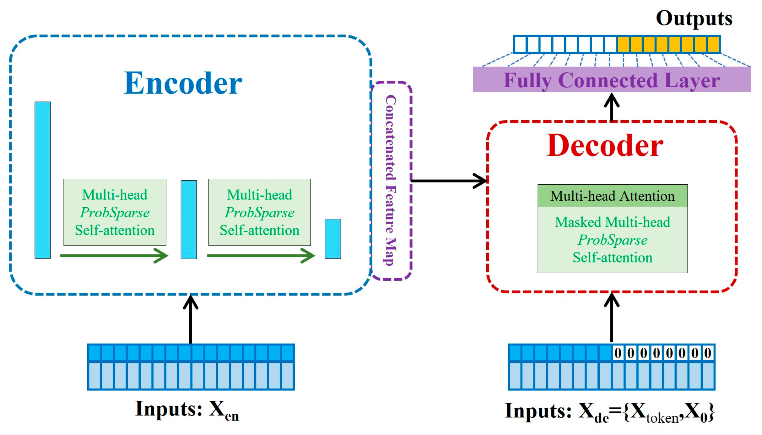
2.1. Informer Algorithm
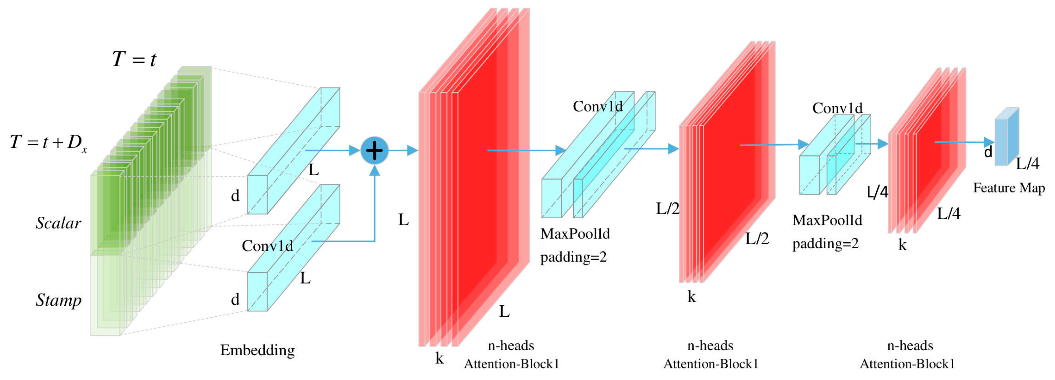
2.2. Improvement of Algorithm Framework
2.3. Improvements Based on Shield Tunneling Characteristics
2.3.1. Soil Layer Classification and Characterization
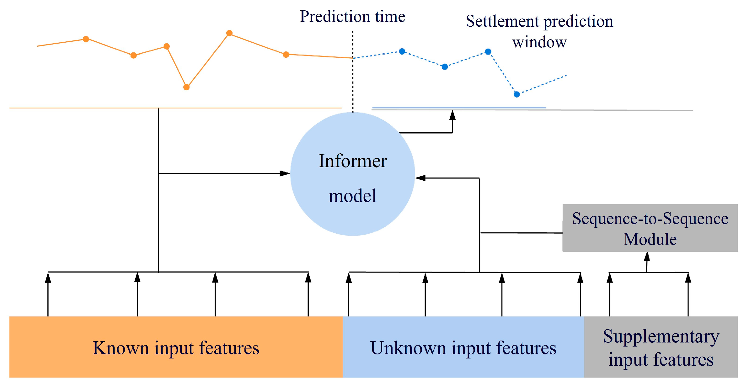
2.3.2. Moving Prediction Window
- (1)
- Known input features (orange blocks in Figure 5): These include shield tunneling parameters (e.g., thrust, cutterhead torque, and advance rate) and geological static parameters (e.g., soil layer classification, density, and compression modulus) monitored before tunneling to the target ring. Their temporal regularity can be captured through historical data.
- (2)
- Unknown input features (blue blocks in Figure 5): These are lagged variables introduced via the moving prediction window, such as settlement values from the past 5–10 rings and displacement trends of shield posture (gray blocks in Figure 5). These features address time-lag effects in settlement prediction.
- (3)
- Supplementary input features (gray blocks in Figure 5): These represent binary indicators (0/1) for abrupt special construction events (e.g., abnormal stoppages and secondary grouting). Their timing and intensity are unpredictable, as detailed in Section 2.3.3.
2.3.3. Special Factor Handling
3. Case Study
3.1. Project Background
3.2. Dataset Construction
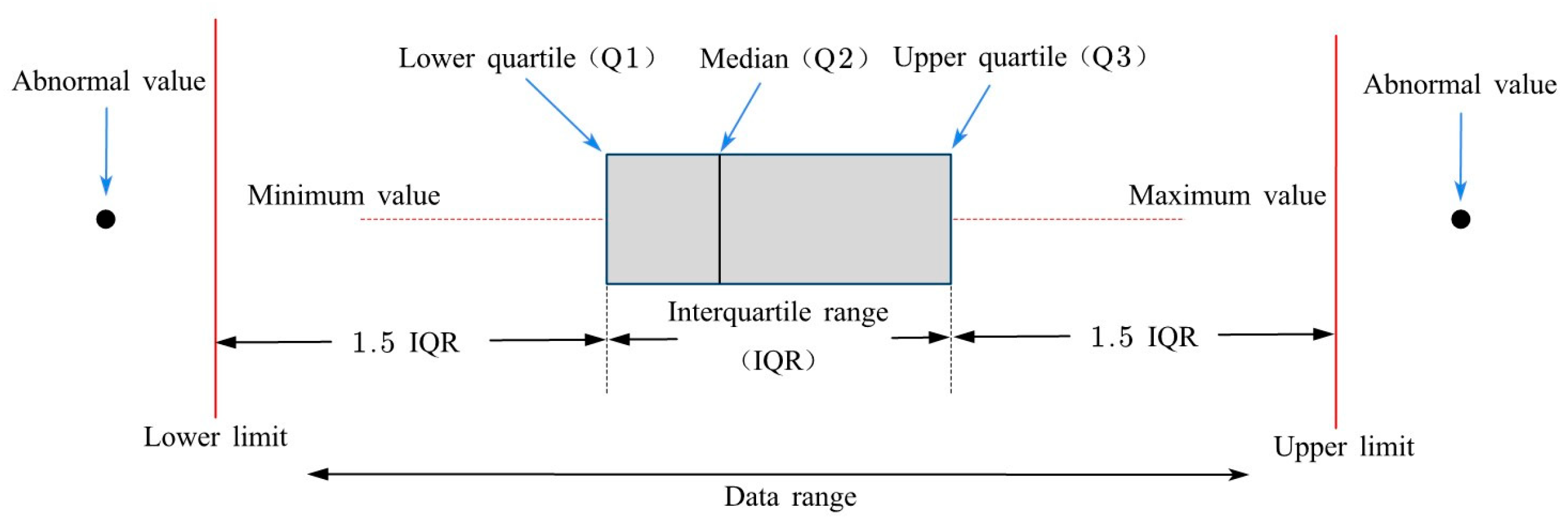
3.3. Data Preprocessing
- (1)
- Data Cleaning
- (2)
- Data Normalization
3.4. Hyperparameter Settings
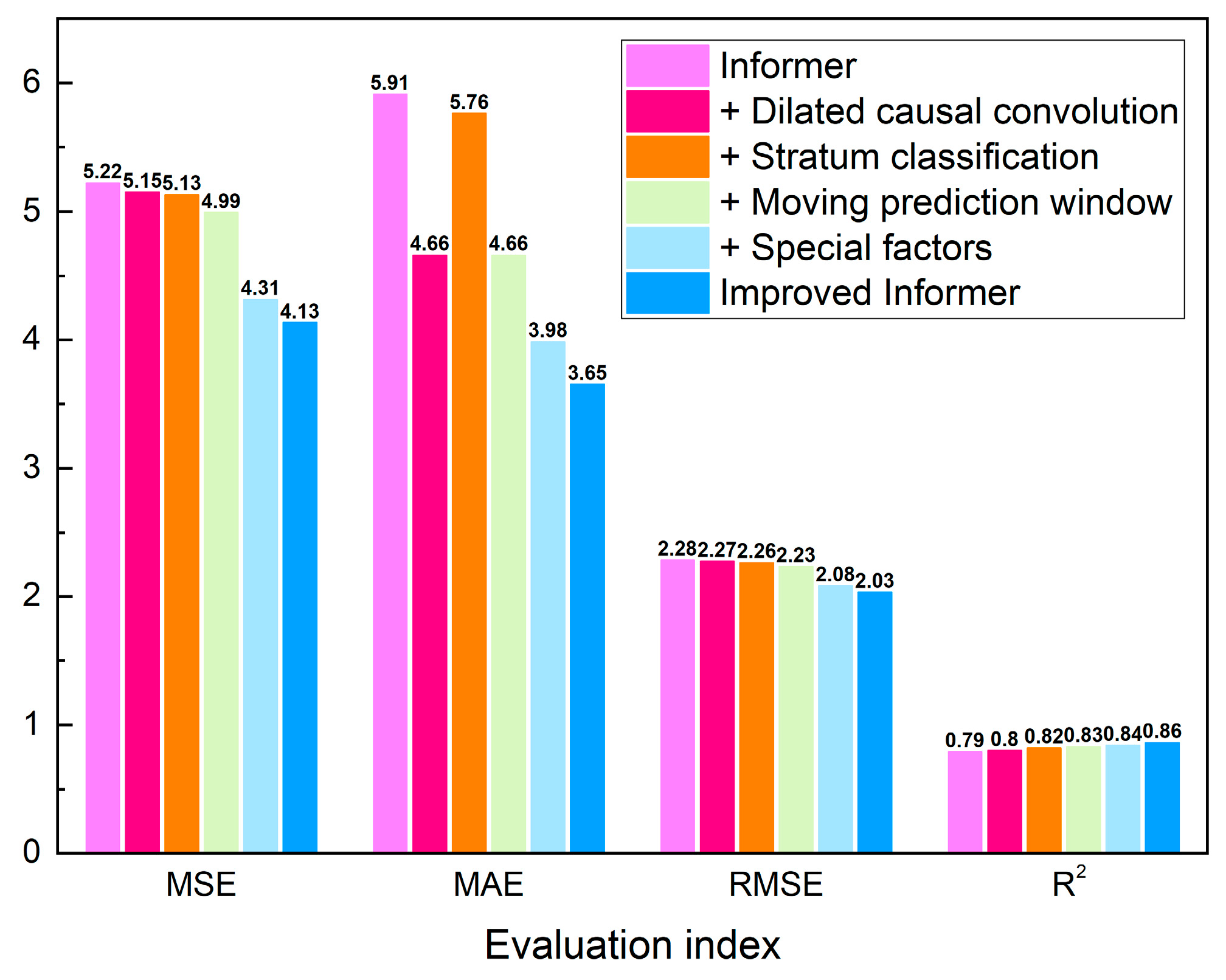
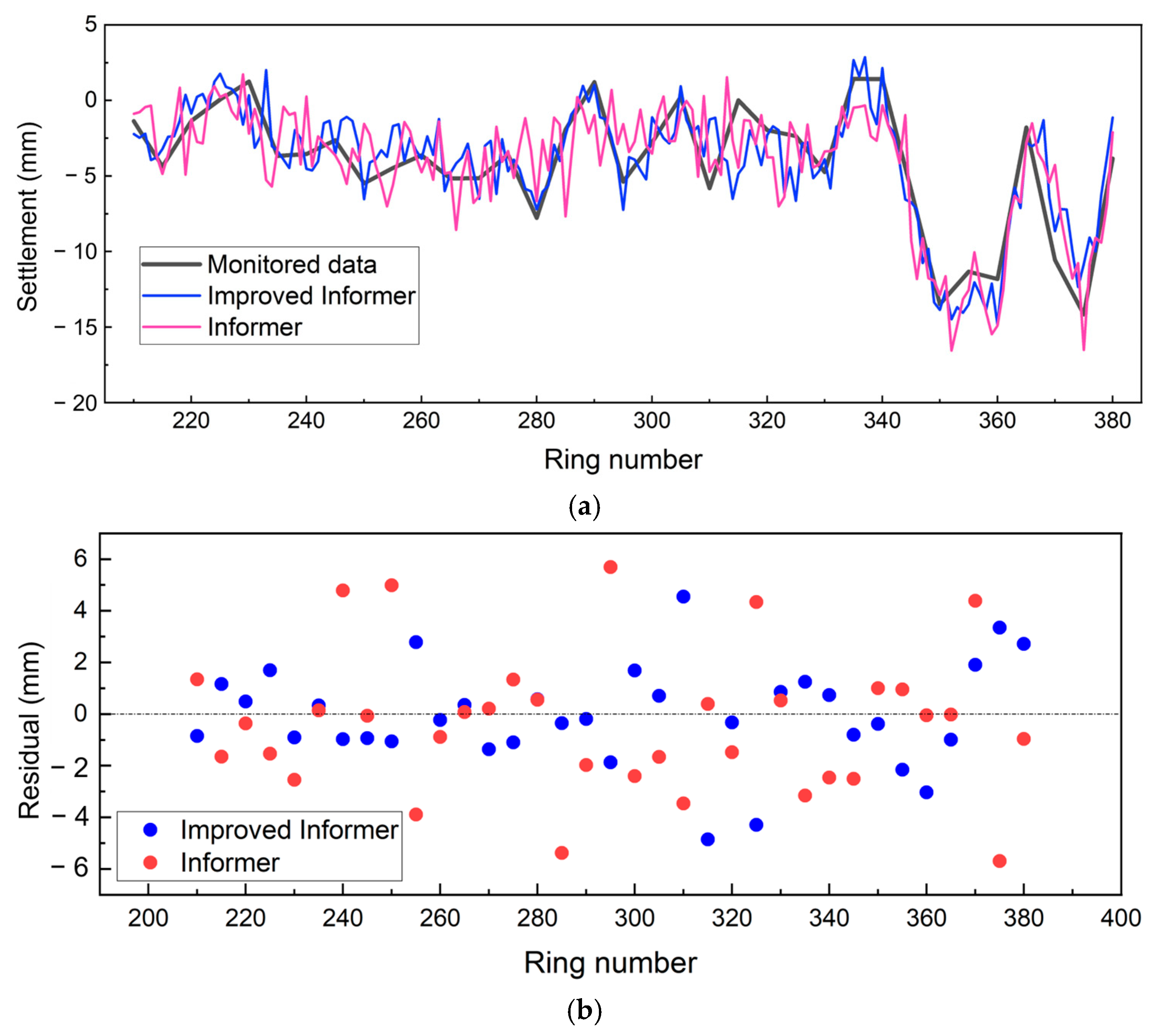
3.5. Comparison of Effects Before and After Improvement
3.5.1. Prediction Accuracy
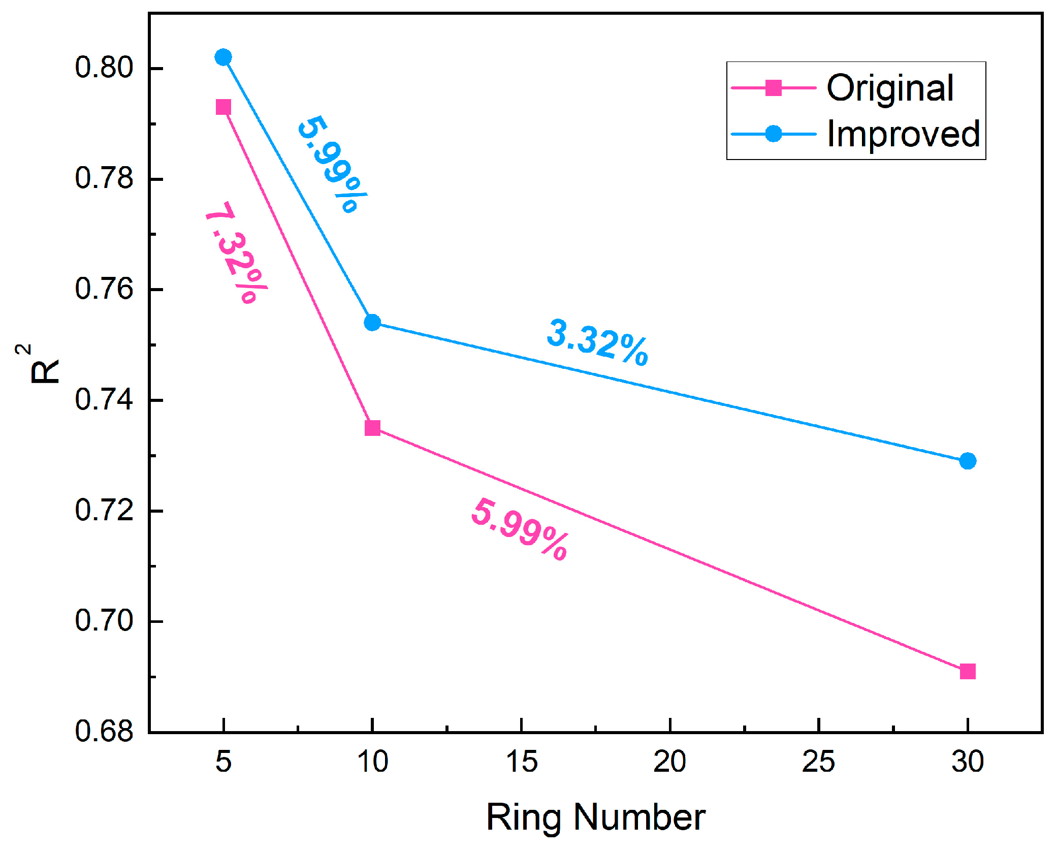
3.5.2. Prediction Accuracy Across Different Timescales
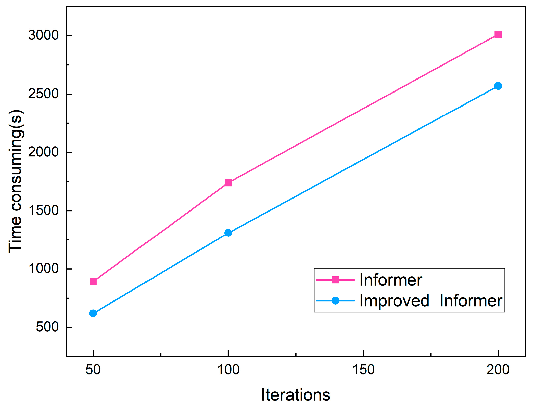
3.5.3. Computational Efficiency
3.6. Comparison with Other Algorithms
3.6.1. Algorithm Descriptions
- (1)
- RF Algorithm
- (2)
- LSTM Algorithm
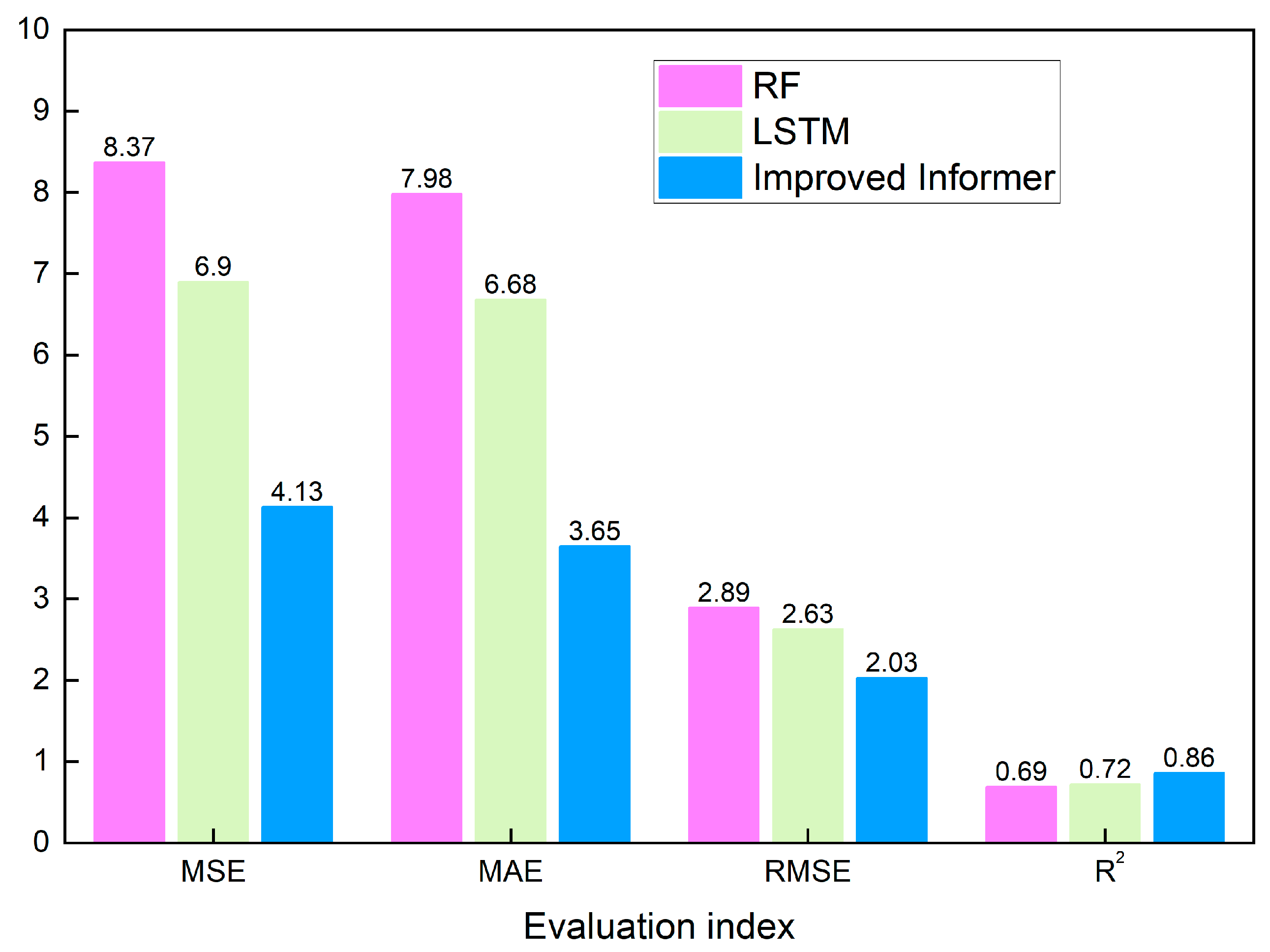
3.6.2. Comparison of Prediction Results
4. Discussion
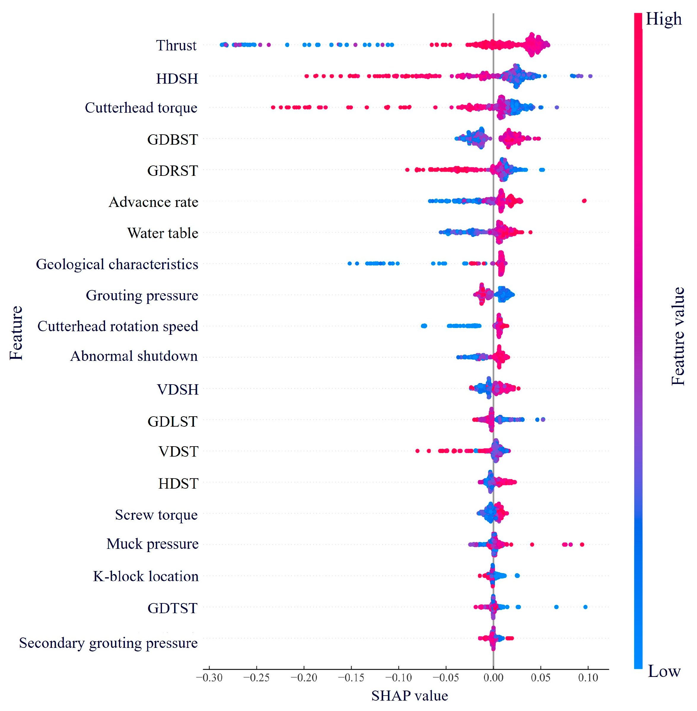
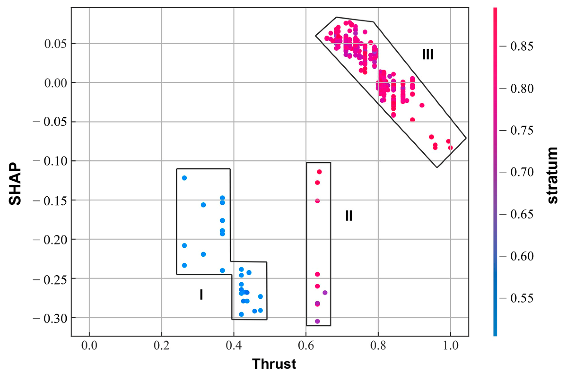
4.1. Analysis of the Influence of Shield Tunneling Features Based on SHAP Theory
4.2. Shield Tunneling Parameter Optimization Design Based on the Multi-Objective Optimization Algorithm
4.3. Model Limitations and Mitigation Pathways
5. Conclusions
- (1)
- To address the limitations of the Informer algorithm in predicting surface settlement, a dilated causal convolutional network was employed to replace the standard convolutional network, and three improvements were made: soil layer classification and characterization, a moving prediction window, and incorporation of special factors. These measures yielded the improved Informer algorithm.
- (2)
- Compared with the original Informer algorithm, the improved Informer algorithm had obvious advantages: ① The prediction accuracy improved significantly. Through the improvements, the R2 value increased from 0.79 to 0.86, the MSE decreased from 5.22 to 4.13, the MAE decreased from 5.91 to 3.65, and the RMSE decreased from 2.28 to 2.03. ② With increasing prediction timescales, the rate of R2 reduction for the improved Informer algorithm was consistently lower than that of the original algorithm. Both the perception range and accuracy of the improved algorithm were optimized. ③ The improved Informer algorithm had a shorter prediction time than the original algorithm. The prediction time was reduced by up to 30.64%. Compared with the RF and LSTM algorithms, the improved Informer algorithm also exhibited superior performance. It is more suitable than other algorithms for predicting surface settlement in metro shield tunneling projects.
- (3)
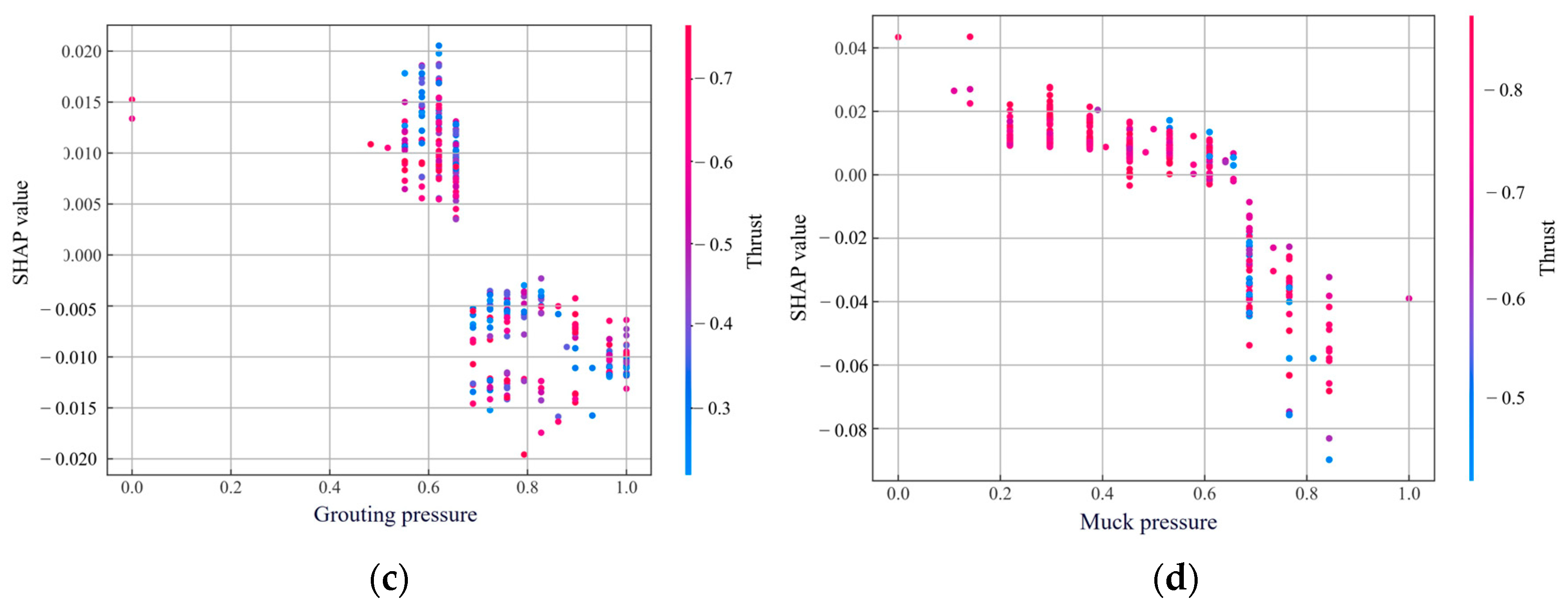
- According to the SHAP theory, we analyzed the effects of shield tunneling parameters on surface settlement. The results indicated that shield thrust was the most critical feature for predicting surface settlement. Its impact on surface settlement needed to be judged in conjunction with soil layer conditions. The cutterhead torque had a negative correlation with its SHAP values. Low tunneling speeds exerted a negative impact on settlement, while high speeds had a positive impact. Additionally, the tunneling speed and thrust exhibited a strong negative correlation. Grouting pressure and muck pressure positively influenced surface settlement at low levels but negatively influenced it at high levels. During the construction process, appropriate increases in thrust torque, grouting pressure, and muck pressure, combined with reduced tunneling speed, were found to effectively mitigate surface settlement.
- (4)
- Shield thrust, cutterhead torque, and tunneling speed were selected as optimization parameters. On this basis, a multi-objective optimization algorithm was developed and solved using the NSGA-III algorithm, with the aim of optimizing the combinations of shield tunneling parameters. Compared with the original tunneling parameters, the optimized combinations reduced surface settlement by 16.79% on average. The optimized parameter combinations effectively controlled surface settlement through multi-objective optimization.
Author Contributions
Funding
Institutional Review Board Statement
Informed Consent Statement
Data Availability Statement
Conflicts of Interest
Appendix A
- (1)
- Shield Tunneling Parameters (19 parameters)
- (2)
- Geological Parameters (14 parameters)
References
- Wei, Y.; Yang, Y.; Tao, M.; Wang, D.; Jie, Y. Earth pressure balance shield tunneling in sandy gravel deposits: A case study of application of soil conditioning. Bull. Eng. Geol. Environ. 2020, 79, 5013–5030. [Google Scholar] [CrossRef]
- Fang, Y.; Yao, Y.; Wang, J.; Li, B.; Dou, L.; Wei, L.; Zhuo, B.; Zhang, W.; Hu, X. Effective dewatering and resourceful utilization of high-viscosity waste slurry through magnetic flocculation. Constr. Build. Mater. 2024, 425, 136014. [Google Scholar] [CrossRef]
- Zumsteg, R.; Langmaack, L. Mechanized tunneling in soft soils: Choice of excavation mode and application of soil-conditioning additives in glacial deposits. Engineering 2017, 3, 863–870. [Google Scholar] [CrossRef]
- Ling, X.; Kong, X.; Tang, L.; Zhao, Y.; Tang, W.; Zhang, Y. Predicting earth pressure balance (EPB) shield tunneling-induced ground settlement in compound strata using random forest. Transp. Geotech. 2022, 35, 100771. [Google Scholar] [CrossRef]
- Chen, R.; Zhang, P.; Kang, X.; Zhong, Z.; Liu, Y.; Wu, H. Prediction of maximum surface settlement caused by earth pressure balance (EPB) shield tunneling with ANN methods. Soils Found. 2019, 59, 284–295. [Google Scholar] [CrossRef]
- Rong, X.; Gao, L.; Han, A.; Wu, J.; Wu, X.; Jiang, G. Analysis of ground volume loss for EPB shield tunneling in thick silty clay layer. Alex. Eng. J. 2024, 96, 295–302. [Google Scholar] [CrossRef]
- Li, C.; Dias, D. Intelligent prediction and visual optimization of surface settlement induced by earth pressure balance shield tunneling. Tunn. Undergr. Space Technol. 2024, 154, 106138. [Google Scholar] [CrossRef]
- Wang, J.; Feng, K.; Wang, Y.; Lin, G.; He, C. Soil disturbance induced by EPB shield tunnelling in multilayered ground with soft sand lying on hard rock: A model test and DEM study. Tunn. Undergr. Space Technol. 2022, 130, 104738. [Google Scholar] [CrossRef]
- Kong, X.; Ling, X.; Tang, L.; Tang, W.; Zhang, Y. Random forest-based predictors for driving forces of earth pressure balance (EPB) shield tunnel boring machine (TBM). Tunn. Undergr. Space Technol. 2022, 122, 104373. [Google Scholar] [CrossRef]
- Lai, H.; Zhang, J.; Zhang, L.; Chen, R.; Yang, W. Anew method based on centrifuge model test for evaluating ground settlement induced by tunneling. KSCE J. Civ. Eng. 2019, 23, 2426–2436. [Google Scholar] [CrossRef]
- Li, S.; Wang, M. Elastic analysis of stress–displacement field for a lined circular tunnel at great depth due to ground loads and internal pressure. Tunn. Undergr. Space Technol. 2008, 23, 609–617. [Google Scholar] [CrossRef]
- Wang, Z.; Shi, C.; Chen, H.; Peng, Z.; Sun, Y.; Zheng, X. Probabilistic analysis of the longitudinal performance of shield tunnels based on a simplified finite element procedure and its surrogate model considering spatial soil variability. Comput. Geotech. 2023, 162, 105662. [Google Scholar] [CrossRef]
- Li, J.; Liu, A.; Xing, H. Study on ground settlement patterns and prediction methods in super-large-diameter shield tunnels constructed in composite strata. Appl. Sci. 2023, 13, 10820. [Google Scholar] [CrossRef]
- Chen, Z.; Zhang, Y.; Li, J.; Li, X.; Jing, L. Diagnosing tunnel collapse sections based on TBM tunneling big data and deep learning: A case study on the Yinsong Project, China. Tunn. Undergr. Space Technol. 2021, 108, 103700. [Google Scholar] [CrossRef]
- Fu, Y.; Chen, L.; Xiong, H.; Chen, X.; Lu, A.; Zeng, Y.; Wang, B. Data-driven real-time prediction for attitude and position of super-large diameter shield using a hybrid deep learning approach. Undergr. Space 2024, 15, 275–297. [Google Scholar] [CrossRef]
- Alsirawan, R.; Sheble, A.; Alnmr, A. Two-dimensional numerical analysis for TBM tunneling-induced structure settlement: A proposed modeling method and parametric study. Infrastructures 2023, 8, 88. [Google Scholar] [CrossRef]
- Editorial Department of China Journal of Highway and Transport. Review on China’s traffic tunnel engineering research: 2022. China J. Highw. Transp. 2022, 35, 1–40. [Google Scholar] [CrossRef]
- Salimi, A.; Faradonbeh, R.S.; Monjezi, M.; Moormann, C. TBM performance estimation using a classification and regression tree (CART) technique. Bull. Eng. Geol. Environ. 2018, 77, 429–440. [Google Scholar] [CrossRef]
- Zhang, W.; Li, H.; Wu, C.; Li, Y.; Liu, Z.; Liu, H. Soft computing approach for prediction of surface settlement induced by earth pressure balance shield tunneling. Undergr. Space 2021, 6, 353–363. [Google Scholar] [CrossRef]
- Tang, L.; Na, S. Comparison of machine learning methods for ground settlement prediction with different tunneling datasets. J. Rock Mech. Geotech. Eng. 2021, 13, 1274–1289. [Google Scholar] [CrossRef]
- Huang, H.; Chang, J.; Zhang, D.; Zhang, J.; Wu, H.; Li, G. Machine learning-based automatic control of tunneling posture of shield machine. J. Rock Mech. Geotech. Eng. 2022, 14, 1153–1164. [Google Scholar] [CrossRef]
- Duan, X. Settlement prediction of Nanjing Metro Line 10 with HOA-VMD-LSTM. Measurement 2025, 244, 116477. [Google Scholar] [CrossRef]
- Wen, K.; Liang, Q. TM-Informer-Based prediction for railway ground surface settlement. J. Circuits Syst. Comput. 2024, 33, 2450316. [Google Scholar] [CrossRef]
- Chang, J.; Huang, H.; Thewes, M.; Zhang, D.; Wu, H. Data-based postural prediction of shield tunneling via machine learning with physical information. Comput. Geotech. 2024, 174, 106584. [Google Scholar] [CrossRef]
- Pourtaghi, A.; Lotfollahi-Yaghin, M.A. Wavenet ability assessment in comparison to ANN for predicting the maximum surface settlement caused by tunneling. Tunn. Undergr. Space Technol. 2012, 28, 257–271. [Google Scholar] [CrossRef]
- Zhou, H.; Zhang, S.; Peng, J. Informer: Beyond efficient transformer for long sequence time-series forecasting. arXiv 2021. [Google Scholar] [CrossRef]
- Lai, J.; Zhu, J.; Guo, Y.; Xie, Y.; Hu, Y.; Wang, P. Amulti-factor-driven approach for predicting surface settlement caused by the construction of subway tunnels by undercutting method. Environ. Earth Sci. 2024, 83, 442. [Google Scholar] [CrossRef]
- Zhao, J.; Ding, X. Predicting tunnel boring machine performance with the Informer model: A case study of the Guangzhou Metro Line project. J. Zhejiang Univ.-Sci. A 2025, 26, 226–237. [Google Scholar] [CrossRef]
- Wang, Z.; Bai, X. Long-term Time Series Prediction of Deformation in the Area of Pylons by Combining InSAR and Transformer-based. In Proceedings of the 2022 Euro-Asia Conference on Frontiers of Computer Science and Information Technology (FCSIT), Beijing, China, 16–18 December 2022; pp. 59–62. [Google Scholar] [CrossRef]
- Hu, M.; Cheng, P. Long-Distance Shield Tunnelling Performance Prediction Based on Informer. Appl. Sci. 2025, 15, 1674. [Google Scholar] [CrossRef]
- Zhen, J.; Huang, M.; Li, S.; Xu, K.; Zhao, Q. Long-Term Forecasting of Shield Tunnel Position and Attitude Deviation Using the 1DCNN-Informer Method. Eng. Sci. Technol. Int. J. 2025, 63, 101957. [Google Scholar] [CrossRef]
- Pang, S.; Hua, W.; Fu, W.; Liu, X.; Ni, X. Multivariable real-time prediction method of tunnel boring machine operating parameters based on spatio-temporal feature fusion. Adv. Eng. Inform. 2024, 62, 102924. [Google Scholar] [CrossRef]
- Zhu, Q.; Han, J.; Chai, K.; Zhao, C. Time series analysis based on Informer algorithms: A survey. Symmetry 2023, 15, 951. [Google Scholar] [CrossRef]
- Cao, J.; Liu, F.; Shen, Z. ALSTM-based model for TBM performance prediction and the effect of rock mass grade on prediction accuracy. China Civ. Eng. J. 2022, 55, 92–102. [Google Scholar] [CrossRef]
- Zhang, P.; Chen, R.; Wu, H.; Liu, Y. Ground settlement induced by tunneling crossing interface of water-bearing mixed ground: A lesson from Changsha, China. Tunn. Undergr. Space Technol. 2020, 96, 103224. [Google Scholar] [CrossRef]
- Rhodes, J.S.; Cutler, A.; Moon, K.R. Geometry- and accuracy-preserving random forest proximities. IEEE Trans. Pattern Anal. Mach. Intell. 2023, 45, 10947–10959. [Google Scholar] [CrossRef]
- Hochreiter, S.; Schmidhuber, J. Long short-term memory. Neural Comput. 1997, 9, 1735–1780. [Google Scholar] [CrossRef]
- Zhang, P.; Wu, H.; Chen, R.; Chan, T.H.T. Hybrid meta-heuristic and machine learning algorithms for tunneling-induced settlement prediction: A comparative study. Tunn. Undergr. Space Technol. 2020, 99, 103383. [Google Scholar] [CrossRef]


| Stratum No. | Stratum | Density, ρ (g/cm3) | Moisture Content, w (%) | Cohesion, c (kPa) | Internal Friction Angle, Φ (°) | Compression Modulus, E (MPa) | Permeability Coefficient, k (m/d) |
|---|---|---|---|---|---|---|---|
| ①1 | Plain fill | 1.88 | 23.1 | 12 | 10 | - | 0.5 |
| ①2 | Miscellaneous fill | 1.90 | 20 | 15 | 5 | - | 2 |
| ③1 | Silty clay | 1.92 | 23.9 | 37.9 | 13.7 | 5.34 | 0.009 |
| ③2 | Silty soil | 1.94 | 21.6 | 10.5 | 19.9 | 8.55 | 0.19 |
| ③3 | Fine sand | 1.97 | - | 5 | 20 | 13 | - |
| ③5 | Medium sand | 2.01 | - | 5 | 25 | 15 | - |
| ⑦1 | Silty clay | 1.93 | 27.5 | 19.9 | 11.7 | 5.56 | 0.0011 |
| ⑨1 | Silty clay | 1.98 | 23.7 | 35.7 | 13.2 | 5.81 | 0.0019 |
| ⑨3 | Silty soil | 1.89 | 26.7 | 42.4 | 13.4 | 6.02 | 0.0093 |
| ⑨6 | Pebble | 2.08 | - | 5 | 40 | 35 | 3.97 |
| ⑨7 | Medium sand | 2.01 | - | 5 | 30 | 15 | 3.97 |
| Parameter | Unit | Mean Value | Standard Deviation | Min. | Max. | 25% | 50% | 75% |
|---|---|---|---|---|---|---|---|---|
| Grouting pressure | bar | 2.62 | 0.45 | 0.4 | 3.3 | 2.3 | 2.6 | 3 |
| K-block location | - | 6.65 | 3.91 | 1 | 15 | 3 | 5 | 11 |
| Horizontal displacement of shield head (HDSH) | mm | −8.74 | 16.30 | −45 | 49 | −21 | −9 | 0 |
| Horizontal displacement of shield tail (HDST) | mm | 3.62 | 18.15 | −45 | 50 | −9 | 1.5 | 16 |
| Vertical displacement of shield head (VDSH) | mm | −34.15 | 8.53 | −50 | 10 | −40 | −35 | −30 |
| Vertical displacement of shield tail (VDST) | mm | −22.72 | 13.05 | −48 | 48 | −30 | −25 | −19 |
| Gap distance at top of shield tail (GDTST) | mm | 51.65 | 7.55 | 28 | 75 | 45 | 50 | 55 |
| Gap distance at bottom of shield tail (GDBST) | mm | 71.63 | 9.58 | 45 | 100 | 65 | 70 | 80 |
| Gap distance at left of shield tail (GDLST) | mm | 70.46 | 9.17 | 40 | 114 | 65 | 70 | 75 |
| Gap distance at right of shield tail (GDRST) | mm | 62.48 | 11.35 | 31 | 95 | 55 | 60 | 70 |
| Screw conveyor rotation speed | r/min | 7.60 | 1.35 | 1 | 10.5 | 7 | 8 | 8.5 |
| Screw conveyor torque | kN·m | 39.41 | 13.59 | 15 | 83 | 28 | 36 | 48 |
| Muck pressure | bar | 1.69 | 0.24 | 0.3 | 2.2 | 1.6 | 1.7 | 1.85 |
| Advanced rate | mm/min | 41.29 | 7.58 | 5 | 55 | 38 | 43 | 48 |
| Volume of excavated earth | m3 | 62.74 | 0.78 | 61 | 65 | 63 | 63 | 63 |
| Cutterhead rotation speed | r/min | 1.19 | 0.09 | 1 | 1.4 | 1.1 | 1.2 | 1.3 |
| Cutterhead torque | kN·m | 2332.18 | 356.64 | 385 | 3531 | 2150 | 2350 | 2500 |
| Grouting volume | m3 | 6.21 | 0.29 | 2.5 | 7.2 | 6.1 | 6.2 | 6.3 |
| Thrust | kN | 11,346.92 | 1083.19 | 4800 | 13,400 | 11,100 | 11,500 | 11,900 |
| Segment No. | Start Ring | End Ring | Total Rings | Role |
|---|---|---|---|---|
| 1 | 1 | 45 | 45 | Training |
| 2 | 46 | 120 | 75 | Training |
| 3 | 121 | 175 | 55 | Test |
| 4 | 176 | 250 | 75 | Training |
| 5 | 251 | 315 | 65 | Training |
| 6 | 316 | 375 | 60 | Training |
| 7 | 376 | 430 | 55 | Test |
| 8 | 431 | 500 | 70 | Training |
| 9 | 501 | 560 | 60 | Training |
| 10 | 561 | 630 | 70 | Training |
| 11 | 631 | 700 | 70 | Training |
| 12 | 721 | 770 | 65 | Test |
| 13 | 771 | 830 | 60 | Training |
| 14 | 831 | 875 | 45 | Training |
| Hyperparameter | Hyperparameter Optimization Range | Optimal Value |
|---|---|---|
| enc_layers | [2, 3] | 2 |
| dec_layers | [1, 3] | 2 |
| n_heads | [2, 8] | 3 |
| e_layers | [1, 2] | 2 |
| d_ff | [128, 512] | 174 |
| factor | [1, 5] | 3 |
| dropout | [0.0, 0.5] | 0.3 |
| embed | [‘fixed’, ‘learned’] | ‘learned’ |
| activation | [‘relu’, ‘gelu’] | ‘gelu’ |
| Improvement Measure | MSE | MAE | RMSE | R2 | Memory (GB) |
|---|---|---|---|---|---|
| Baseline (Original Informer) | 5.22 | 5.91 | 2.28 | 0.79 | 3.2 |
| + Dilated Causal Convolution | 5.15 | 4.66 | 2.27 | 0.80 | 3.0 |
| + Stratum Classification | 5.13 | 5.76 | 2.26 | 0.82 | 2.2 |
| + Moving Prediction Window | 4.99 | 4.66 | 2.23 | 0.83 | 2.3 |
| + Special Factors | 4.31 | 3.98 | 2.08 | 0.84 | 2.3 |
| Hyperparameter | Hyperparameter Optimization Range | Optimal Value |
|---|---|---|
| n_estimators | [2, 50] | 17 |
| criterion | [‘gini’, ‘entropy’] | ‘gini’ |
| max_depth | [1, 15] | 6 |
| min_samples_split | [2, 10] | 2 |
| min_samples_leaf | [1, 4] | 1 |
| min_weight_fraction_leaf | [0, 0.5] | 0.1 |
| Hyperparameter | Hyperparameter Optimization Range | Optimal Value |
|---|---|---|
| units | [50, 200] | 155 |
| activation | [‘relu’, ‘tanh’] | ‘tanh’ |
| recurrent_activation | [‘sigmoid’] | ‘sigmoid’ |
| use_bias | [True, False] | True |
| kernel_initializer | [‘glorot_unifo rm’, ‘he_uniform’] | ‘glorot_uniform’ |
| recurrent_initializer | [‘orthogonal’] | ‘orthogonal’ |
| bias_initializer | [‘zeros’] | ‘zeros’ |
| unit_forget_bias | [True, False] | True |
| dropout | [0.0, 0.5] | 0.2 |
| recurrent_dropout | [0.0, 0.5] | 0.2 |
| Combination of Excavation Parameters | Thrust (kN) | Cutterhead Torque (kN·m) | Advance Rate (mm/min) | Settlement (mm) |
|---|---|---|---|---|
| Original | 11,300 | 2460.9982 | 39.0000 | −10.247 |
| 11,500 | 2337.2135 | 40.0000 | 2.171 | |
| 11,500 | 2311.4430 | 42.0000 | −7.520 | |
| 11,300 | 2201.9703 | 45.0000 | −4.071 | |
| 11,700 | 2317.9262 | 47.0000 | −6.315 | |
| Optimized | 11,714 | 2449.8298 | 38.8373 | 1.2623 |
| 11,402 | 2447.8458 | 40.0938 | −1.2648 | |
| 11,600 | 2352.7812 | 40.3691 | −2.9640 | |
| 11,453 | 2251.7883 | 44.8257 | −0.7665 | |
| 11,732 | 2448.3156 | 45.0416 | −5.1628 |
Disclaimer/Publisher’s Note: The statements, opinions and data contained in all publications are solely those of the individual author(s) and contributor(s) and not of MDPI and/or the editor(s). MDPI and/or the editor(s) disclaim responsibility for any injury to people or property resulting from any ideas, methods, instructions or products referred to in the content. |
© 2025 by the authors. Licensee MDPI, Basel, Switzerland. This article is an open access article distributed under the terms and conditions of the Creative Commons Attribution (CC BY) license (https://creativecommons.org/licenses/by/4.0/).
Share and Cite
Zhao, S.; Feng, X.; Peng, K. Prediction and Parameter Optimization of Surface Settlement Induced by Shield Tunneling Using Improved Informer Algorithm. Appl. Sci. 2025, 15, 6766. https://doi.org/10.3390/app15126766
Zhao S, Feng X, Peng K. Prediction and Parameter Optimization of Surface Settlement Induced by Shield Tunneling Using Improved Informer Algorithm. Applied Sciences. 2025; 15(12):6766. https://doi.org/10.3390/app15126766
Chicago/Turabian StyleZhao, Shisen, Xianda Feng, and Kefeng Peng. 2025. "Prediction and Parameter Optimization of Surface Settlement Induced by Shield Tunneling Using Improved Informer Algorithm" Applied Sciences 15, no. 12: 6766. https://doi.org/10.3390/app15126766
APA StyleZhao, S., Feng, X., & Peng, K. (2025). Prediction and Parameter Optimization of Surface Settlement Induced by Shield Tunneling Using Improved Informer Algorithm. Applied Sciences, 15(12), 6766. https://doi.org/10.3390/app15126766