Comprehensive Optimization of Air Quality in Kitchen Based on Auxiliary Evaluation Indicators

Abstract

Traditional single-scale indoor air quality (IAQ) evaluation methods often fail to meet the demands of modern, personalized kitchens. To address this limitation, we propose a comprehensive IAQ index, integrating experimental data and simulation results. The index incorporates four key IAQ auxiliary evaluation indicators: air distribution performance index (ADPI), predicted mean vote (PMV), cooking oil fume particulates (COFP), and CO₂ concentration. We developed a kitchen model and used the comprehensive IAQ index to benchmark simulation results against experimental tests. Optimal kitchen air quality occurred at a supply air angle of 90° and airflow velocity of 2.268 m³/min, reducing air pollution impact by 29.50%. This configuration enhanced thermal comfort while reducing secondary COFP accumulation in the breathing zone by 22%. The 29.50% Q-index reduction corresponded to a 24% decrease in peak CO₂ exposure (638 ppm, clean-air level) and 22% lower COFP in breathing zones, mitigating health risks. Optimized airflow (2.268 m³/min) avoided excessive ventilation, reducing energy waste and achieving balanced IAQ-energy efficiency.

1. Introduction

With rapid urbanization and modernization, contemporary home kitchens have become increasingly enclosed and compact, leading to concerns over indoor air quality (IAQ). Traditional Chinese cooking methods, which involve high-temperature frying and stir-frying, generate significant amounts of cooking oil fume particulate (COFP) and carbon dioxide (CO₂), both of which pose serious health risks [1,2]. Prolonged exposure to elevated levels of particulate matter and CO₂ can lead to respiratory diseases, discomfort, and long-term health complications. Despite the widespread use of kitchen ventilation systems, the effectiveness of these systems in mitigating air pollutants remains inconsistent, necessitating comprehensive assessment and optimization of IAQ in kitchen environments [3,4,5].

IAQ is a crucial factor affecting human health and well-being [6,7]. Poor ventilation and inadequate air exchange rates exacerbate the accumulation of harmful pollutants in enclosed kitchen spaces, increasing the risks associated with prolonged exposure. Consequently, developing systematic IAQ assessment methods and proposing effective ventilation strategies are imperative. While existing IAQ standards provide general guidelines, they often neglect unique cooking environment characteristics, such as thermal plumes, pollutant dispersion, and occupant exposure levels [8,9].

Several studies have focused on evaluating IAQ through predictive models and experimental assessments. The predicted mean vote (PMV) model, introduced by Fanger [10], has been widely applied in thermal comfort research. Toftum et al. [11] investigated the effects of fabric materials like cotton and polyester on skin thermal sensation under high humidity conditions. Their study demonstrated that variations in indoor relative humidity significantly influenced thermal sensation, leading to the development of a satisfaction model that considers the impact of skin moisture. Kuchen et al. [12] examined thermal comfort across 148 different workspaces in Germany during winter. Their findings indicated that the PMV index closely corresponded with comfort vote values and was highly sensitive to factors such as clothing insulation levels. Buratti et al. [13] applied the tracer gas decay method to assess air age in office environments, validating their numerical model with experimental data using CO₂ as a tracer gas to evaluate IAQ. Further research has explored the effects of environmental factors such as humidity, airflow distribution, and pollutant dispersion on IAQ. For instance, Chen et al. [14] developed a computational fluid dynamics (CFD) framework to model the concentration variations of cooking fumes, assessing both air quality and thermal comfort. Their study analyzed airflow regions around the human body and quantified discomfort using a standardized dissatisfaction metric. Song [15] used ANYSYS 2021R simulation software to compare IAQ under two ventilation systems, namely exhaust and supply air, finding that the air age in rooms with exhaust ventilation was approximately 31.15% lower than those with supply air ventilation. Fan [16] conducted experimental and simulation studies to evaluate humidity, CO₂ concentration, and PMV-PPD (predicted percentage dissatisfied) indices in bedroom environments, revealing that increased indoor relative humidity inhibited pollutant diffusion. Lin et al. [17] employed PIV experiments and CFD simulations to analyze temperature and airflow fields within an aircraft cabin with reduced seat pitch. Their findings indicated that the optimal supply air velocity in this model was 1.35 m/s. Additionally, Wang et al. [18] used AIRPAK software to simulate airflow patterns in ship cabins under different air supply configurations. Their analysis, incorporating PMV, PPD, air age, and temperature fields, demonstrated that cross-ventilation, where supply air enters from one side and return air exits from the opposite side, provided superior indoor conditions. In contrast, when both supply and return air were located on the same side, indoor–outdoor air exchange efficiency significantly declined. Zhang et al. [19] investigated the optimization of make-up air and exhaust rates in commercial kitchens with multiple cookers. Using CFD simulations validated by field tests, the research identifies the optimal make-up air distribution method, which can reduce exhaust rates by up to 20%. Zhang et al. [20] analyzed thermal comfort in kitchens using an air-conditioned range hood. By optimizing airflow distribution, the study improves cooling efficiency and reduces heat exposure during cooking. Li et al. [21] examined the impact of a three-sided slit make-up air system on thermal comfort and air quality in low-energy buildings. The results show that the system reduces PM2.5 and TVOC concentrations while improving temperature control. Optimal operating parameters for pollutant control are also identified, offering insights for improving ventilation in airtight kitchens. Song et al. [22] proposed an exhaust hood with air-filled slots to enhance pollutant capture efficiency. Through numerical simulations and experiments, it determines the optimal slot width and jet velocity for effective pollutant removal. The findings help optimize kitchen exhaust systems, improving indoor air quality and reducing exposure to cooking emissions. Liu et al. [23] presented a novel local ventilation strategy to enhance air quality in residential kitchens by reducing PM2.5 exposure. The study explores factors affecting system performance using CFD simulations and finds that optimized air supply and exhaust configurations can significantly improve pollutant capture efficiency while minimizing occupant exposure. Xie et al. [24] presented a combined range hood and air cleaner system to enhance kitchen air quality and energy efficiency. Simulation and experimental results show that the system effectively reduces PM2.5 and TVOC concentrations while saving energy compared to conventional exhaust-only ventilation. The findings contribute to the design of more effective kitchen ventilation solutions. Wu et al. [25] utilized CFD and a human thermoregulation model to evaluate thermal comfort under different kitchen ventilation modes. Their results show that mechanical ventilation with air curtains significantly improves thermal conditions, reducing temperature fluctuations and increasing comfort by 42%. The findings help optimize ventilation strategies for kitchens in varying climates.

Although previous studies have made significant progress in evaluating IAQ, many have focused on either thermal comfort or pollutant dispersion in isolation, without integrating multiple IAQ factors [26,27]. Additionally, research specifically addressing enclosed kitchens with high-pollutant cooking methods remains scarce. Most studies have examined office spaces, bedrooms, or industrial settings, which differ significantly from residential kitchens in terms of pollutant sources, ventilation patterns, and human exposure levels. Given the growing health concerns associated with indoor air pollution, an integrated approach considering airflow distribution, pollutant concentration, and human comfort is essential to develop optimized ventilation strategies for domestic kitchens [28].

This study introduces a novel methodology for assessing and optimizing kitchen IAQ through combined experimental testing and numerical simulations. Its primary innovation is the development of a comprehensive auxiliary evaluation index, Q, which integrates key IAQ indicators: COFP and CO₂ concentrations, thermal comfort (PMV), and airflow distribution effectiveness (ADPI). Furthermore, the research explores ventilation optimization by analyzing the impact of air supply angles and airflow rates on pollutant removal efficiency. By establishing this holistic IAQ assessment framework and proposing targeted ventilation strategies, this work provides a foundation for improving IAQ in kitchens. While recent studies focus on hybrid ventilation [19,23] or AI-driven optimization [25] for energy efficiency or generic spaces, this work establishes a physics-based, multi-criteria Q-index specifically for kitchens. This integrated approach offers a reproducible framework for deterministic ventilation design, complementing data-driven methods. The practical optimization of supply angle and velocity demonstrates viability without complex sensors or algorithms, addressing gaps in cost-sensitive residential applications.

2. Description of Numerical Method

2.1. Mathematical Model

The fundamental equations of fluid dynamics include the continuity equation, the momentum conservation equation, and the energy conservation equation. These equations describe the time-dependent variations of physical quantities in a fluid, such as velocity and temperature, and are used to analyze flow processes with transient behavior. Mathematically, they are expressed as follows,

Mass conservation equation:

$${\displaystyle \frac{\partial \rho }{\partial t}}+\nabla \left(\rho \overrightarrow{u}\right)=0$$

(1)

Momentum conservation equation:

$${\displaystyle \frac{\partial \overrightarrow{u}}{\partial t}}+\left(\overrightarrow{u}\cdot \nabla \right)\overrightarrow{u}=f-{\displaystyle \frac{1}{\rho }}\nabla p+{\displaystyle \frac{\mu }{\rho }}{\nabla }^2\overrightarrow{u}$$

(2)

Energy conservation equation:

$${\displaystyle \frac{\partial (\rho T)}{\partial t}}+\mathrm{div}(\rho \stackrel{\rightharpoonup }{u}T)=\mathrm{div}\left({\displaystyle \frac{K}{c_p}}\mathrm{grad}T\right)+S_T$$

(3)

where $\rho$ in kg/m³ is the fluid density, $t$ in sec is the time, $u$ in m/s is the velocity vector, $f$ in N is the external force acting on the fluid per unit volume, $p$ in N/m² is the pressure, $\mu$ in N∙s/m² is the dynamic viscosity constant, $T$ in $K$ is the temperature of the kitchen airflow, $K$ in W/(m²∙K) is the heat transfer coefficient in the kitchen, $S_T$ in kg∙K/(m³∙s) is the viscous dissipation term, $c_p$ in J/(kg∙K) is the specific heat. Equations (1)–(3) can be used to calculate the fluid density $\rho$, velocity vector $u$, and temperature $T$.

2.2. Air Quality Evaluation Metrics

Indoor air pollutants are diverse and encompass substances such as carbon dioxide, carbon monoxide, particulate matter, microbial colonies, and formaldehyde. In this study, gaseous CO₂ and solid-phase COFP are selected as the primary evaluation variables. Additionally, PMV and ADPI are incorporated to provide a more comprehensive and integrated assessment of air quality.

2.2.1. Evaluation Index: ADPI

As a comfort rating index, ADPI is used to assess the presence of drafts and evaluate the combined effects of air temperature and velocity on thermal comfort for occupants. A higher ADPI value indicates better air distribution and occupant comfort, with values above 80% generally considered to represent good air distribution. The calculation formula is as follows:

$$\Delta ET=(t_i-t_n)-7.66(u_i-0.15)$$

(4)

$$ADPI={\displaystyle \frac{(-1.7<\Delta ET<1.1)p_i}{p_t}}\times 100\%$$

(5)

where $\Delta ET$ is the effective temperature difference, K; $t_i$ is the temperature at the measurement point, K; $u_i$ is the velocity at the measurement point, m/s; $t_n$ is the temperature in the occupied zone, K; $p_i$ is the number of measurement points that meet the requirements, and $p_t$ is the total number of measurement points.

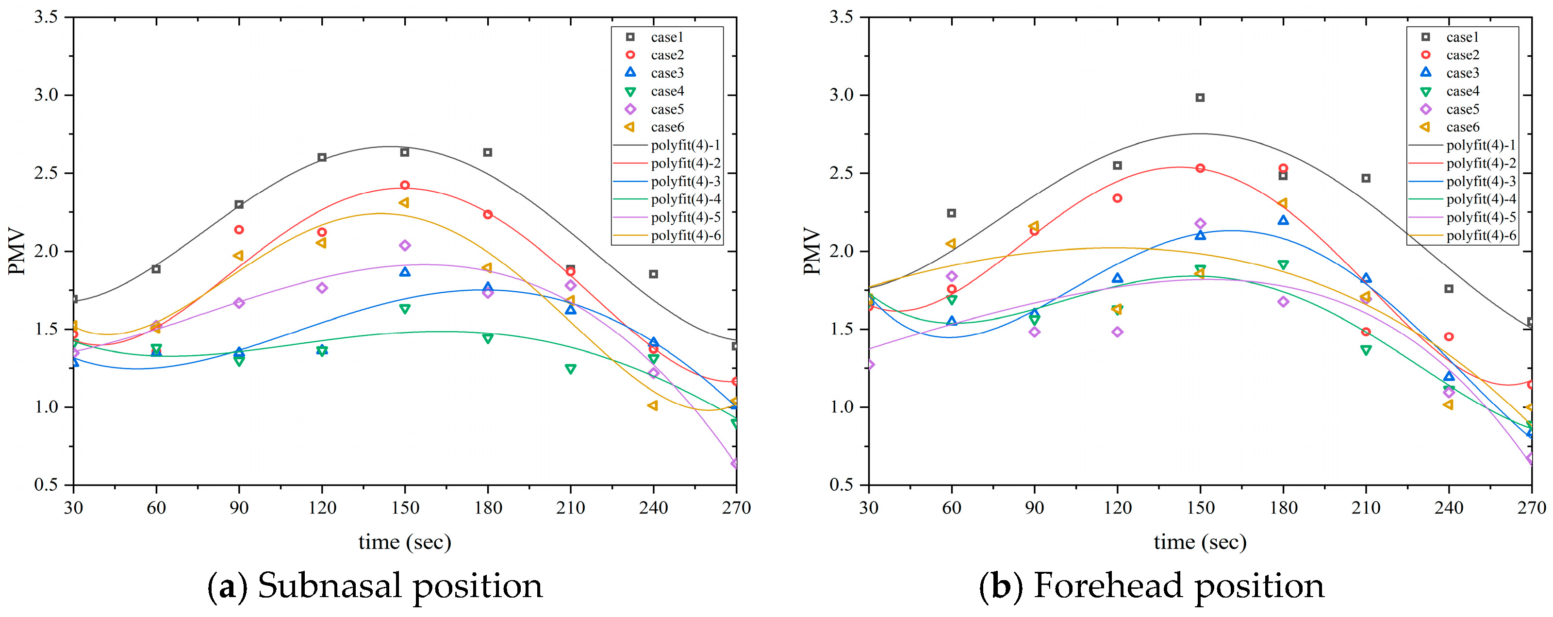
2.2.2. Evaluation Index: PMV

PMV, as a metric for assessing thermal sensation, predicts the average thermal comfort level by accounting for six key factors, namely metabolic rate, clothing insulation, air velocity, humidity, air temperature, and mean radiant temperature. The PMV formulation is expressed as follows:

$$\mathrm{PMV}=\left(0{.0303\mathrm{e}}^{-0.036M}+0.028\right)\left\{\begin{array}{l}\left(M-W\right)-3.05\times {10}^{-3}\times \left[5733-6.99\left(M-W\right)-P_a\right]-\\ 0.42\times \left[\left(M-W-58.15\right)\right]-1.72\times {10}^{-5}M\left(5867-P_a\right)-\\ 0.0014M\left(34-t_a\right)-3.96\times {10}^{-8}{f}_{cl}\times \\ \left[{\left(t_{cl}+273.15\right)}^4-{\left(\overline{t_r}+273.15\right)}^4\right]-f_{cl}{h}_c(t_{cl}-t_a)\end{array}\right.\left.\begin{array}{l}\\ \\ \\ \\ \end{array}\right\}$$

(6)

In the formula: $P_a$ is the metabolic rate, ${\mathrm{W}/\mathrm{m}}^2$; W is the heat consumed by external work (negligible), ${\mathrm{W}/\mathrm{m}}^2$; $P_a$ is the partial pressure of water vapor, Pa; $t_a$ is the air temperature, °C; $f_{cl}$ is the coefficient of human clothing area, which is the ratio of the external surface area of human clothing to its naked surface area.

According to indoor thermal comfort standards, the PMV value should range from −1 to 1 to ensure an acceptable indoor environment.

Table 1. PMV value and thermal sensation scale.

Sensation Description	Hot	Warm	Slightly Warm	Neutral	Slightly Cool	Cool	Cold
PMV Value	+3	+2	+1	0	−1	−2	−3

presents the relationship between PMV values and the corresponding thermal sensation indices.

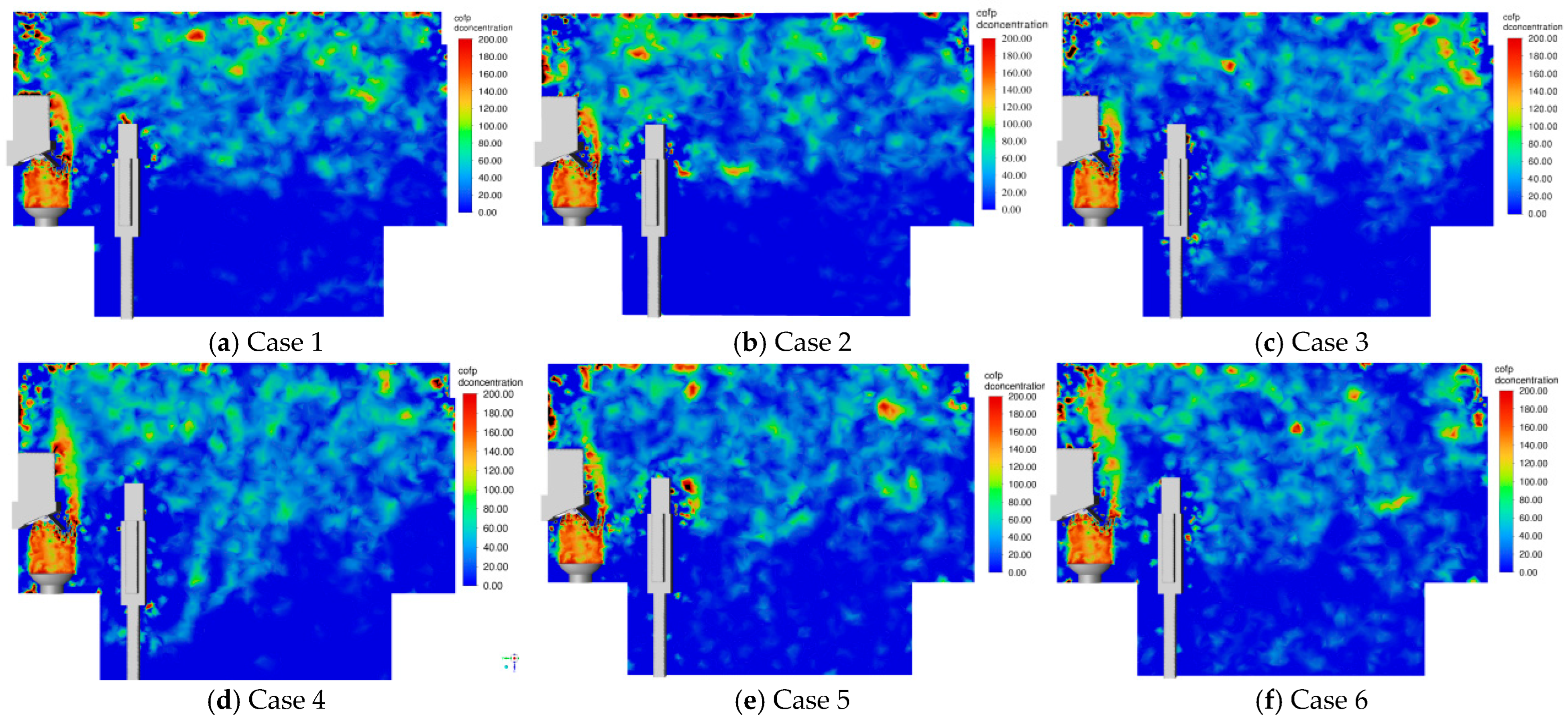
2.2.3. Evaluation Index: Inhalable Particulate Matter

In the present study COFP is represented by inhalable particulate matter (PM₁₀). The World Health Organization (WHO) established a unified indoor air quality standard for PM₁₀ concentrations as early as 2007, which is categorized into four stages: IT-1, IT-2, IT-3, and the guideline value.

Table 2. WHO Standards for inhalable particulate matter concentration.

Transition Stage	${\mathbf{PM}}_{10} \mathbf{Concentration}$(μg/m3)		Indicate
IT-1	Annual Average	70	Initial target value, suitable for areas with poor air quality, aimed at gradually reducing PM10 concentrations.
	Daily Average	150
IT-2	Annual Average	50	A more stringent target, suitable for areas that have reached the IT-1 standard, encouraging further reduction of PM10 pollution.
	Daily Average	100
IT-3	Annual Average	30	A higher target value, aimed at further improving air quality, suitable for regions that have achieved the IT-2 standard.
	Daily Average	57
Guideline	Annual Average	20	The ultimate goal, based on epidemiological studies, aimed at minimizing the health risks associated with PM10 exposure.
	Daily Average	50

shows the details of the standards. The objective of this study is to meet the guideline value.

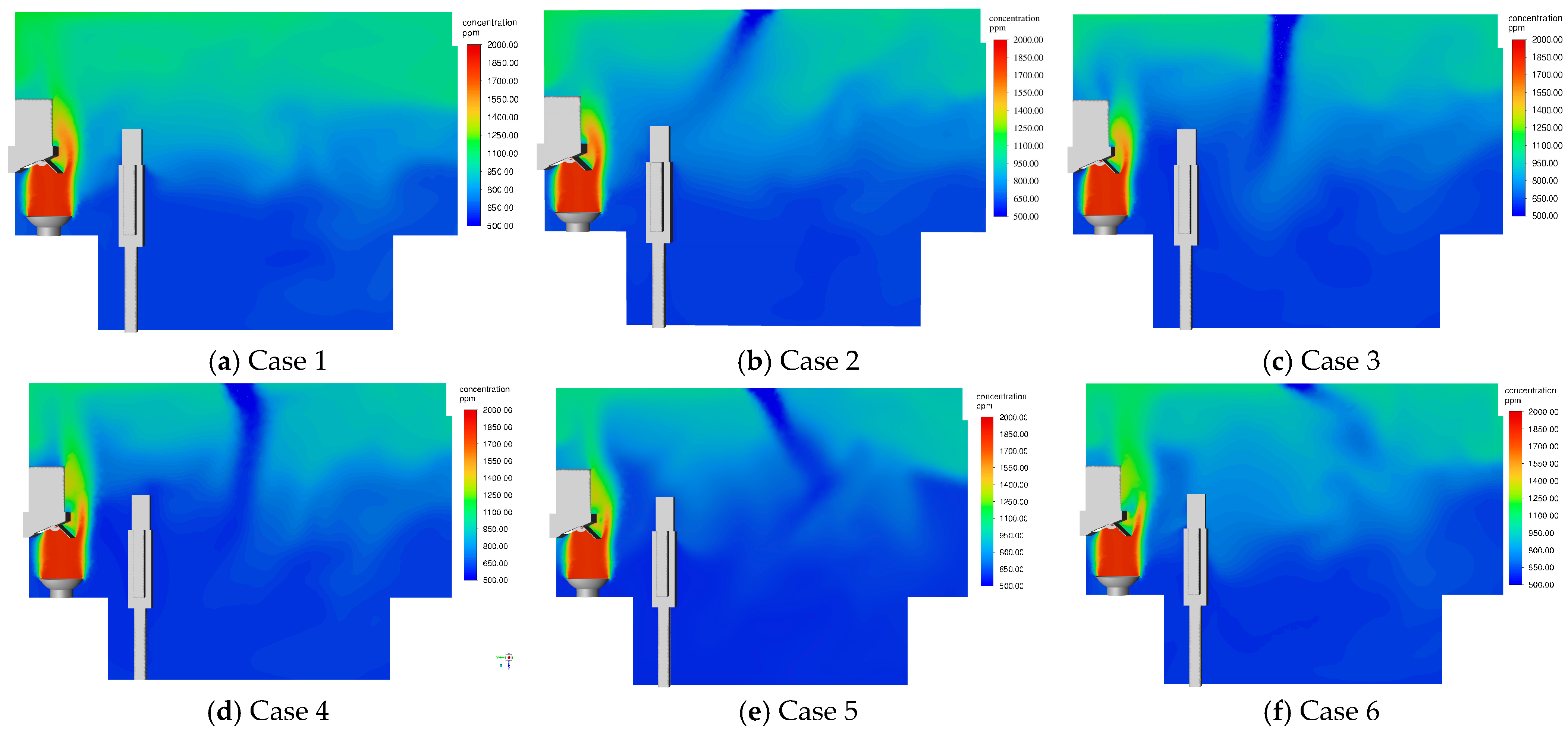
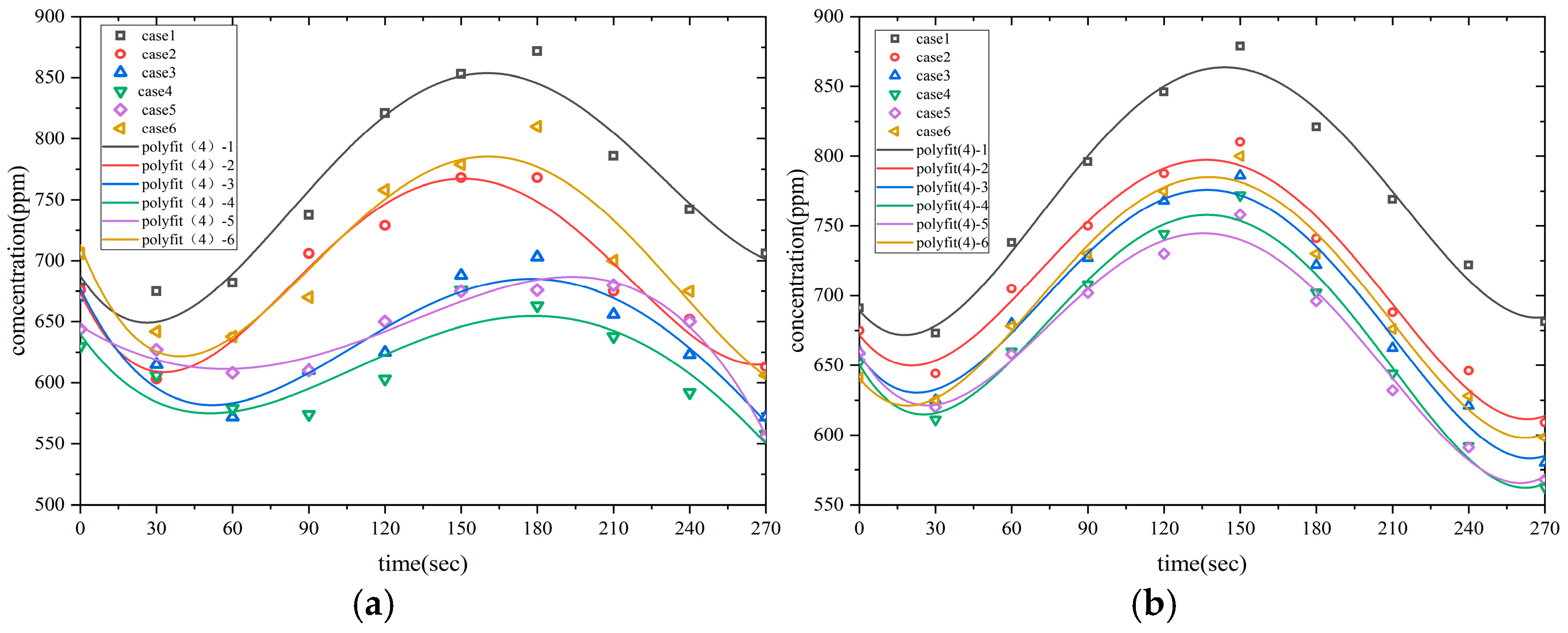
2.2.4. Evaluation Index: CO₂ Concentration

CO₂ is one of the most prevalent indoor pollutants, primarily originating from human respiration and the use of cooking appliances in kitchen environments. Elevated concentration of CO₂ can rapidly and directly impact human comfort and health.

Table 3. CO₂ concentration limits and associated hazards.

CO2 Concentration/ppm	Air Pollution Level	Hazard
<700	Clean air	None
700~1000	Meets hygienic standards	Unpleasant odour
1000~1500	Mild pollution	Air deterioration, discomfort for occupants
1500~2000		Discomfort for most occupants
2000~3000	Severe pollution	Respiratory discomfort
3000~4000		Headache, tinnitus, eye irritation
>8000		Respiratory distress, lethargy, severe cases may lead to death

outlines the standards for different CO₂ concentrations and their associated health risks. The objective of this study is to meet the clean air standard.

2.3. Application of the Auxiliary Evaluation Index

To comprehensively assess indoor air quality during kitchen cooking, this study introduces an auxiliary evaluation index, Q. This index provides a unified framework for integrating multiple air quality indicators, including ADPI, PMV, COFP, and CO₂, enabling a holistic evaluation of indoor environments. This section defines, refines, and explores the application of Q, laying the foundation for subsequent experimental and numerical validations.

2.3.1. Initial Definition and Limitations

Initially, Q is defined as the arithmetic average of several normalized air quality indicators. Each indicator’s measured value is divided by its standard upper limit, resulting in a dimensionless summation index. The formula is expressed as follows:

$$Q=\frac{1}{4}({\displaystyle \frac{100\% ADPI}{20\%}}+{\displaystyle \frac{PMV}{1}}+{\displaystyle \frac{C{O}_2}{700}}+{\displaystyle \frac{COFP}{50}})$$

(7)

Although this approach provides a straightforward method for integrating diverse metrics, it has several limitations. Firstly, the variations in individual indicators affect the overall Q value inconsistently. Secondly, the negative PMV values, which indicate thermal discomfort, are not adequately accounted for. Thirdly, assigning equal weights to all indicators fails to reflect their relative importance.

2.3.2. Improved Formulation

To address the limitations of the initial Q-index (Equation (7)), an improved formulation is proposed. This revision focuses on three key enhancements: first, handling negative PMV values (indicating thermal discomfort) by using its absolute value to ensure consistent representation of discomfort magnitude; second, introducing weighting coefficients (A, B, C, D) to reflect the relative importance of each constituent indicator; and third, reconciling the inconsistent directional impacts of individual indicators on the composite index to ensure uniform interpretation of their influence.

$$Q=\mathrm{A}{\displaystyle \frac{100\%-\mathrm{ADPI}}{20\%}}+B{\displaystyle \frac{\left|PMV\right|}{1}}+C{\displaystyle \frac{C{O}_2}{700}}+D{\displaystyle \frac{COFP}{50}}$$

(8)

where A + B + C + D = 1.

(1) Determining Weighting Coefficients

The weights A, B, C, D are derived based on the contribution of each indicator’s variation range to the total variability of Q. This ensures balanced influence across metrics. For each indicator i, compute its normalized contribution $K_i$.

$$K_i={\displaystyle \frac{|Q_{i\mathit{max}}-Q_{i\mathit{min}}|}{{\displaystyle \sum |Q_{i\mathit{max}}-Q_{i\mathit{min}}|}}}, i\in \left\{C{O}_2,COFP,ADPI,PMV\right\}$$

(9)

Here, $Q_{i\mathit{max}}$ and $Q_{i\mathit{min}}$ are the maximum and minimum values of Q when only indicator $i$ varies within its standard range, while others are fixed at baseline values (per international standards).

To equalize the contributions of all indicators to $Q$, the weights A, B, C, D satisfy:

$$A\times K_{C{O}_2}=B\times K_{ADPI}=C\times K_{PMV}=D\times K_{COFP}$$

(10)

This ensures uniform sensitivity of Q to changes in each indicator.

(2) Taking the ADPI calculation as an example, according to international standards, ADPI has a maximum value of 100% and a minimum of 0. When determining ADPI’s contribution to Q, all other parameters adopt baseline values specified in international standards. Consequently, the contribution of ADPI to Q is calculated as follows:

$$\begin{array}{l}{Q}_{\mathit{max}}=({\displaystyle \frac{100\%-0}{20\%}}+{\displaystyle \frac{1}{1}}+{\displaystyle \frac{700}{700}}+{\displaystyle \frac{50}{50}})=8\\ Q_{\mathit{min}}=({\displaystyle \frac{100\%-100\%}{20\%}}+{\displaystyle \frac{1}{1}}+{\displaystyle \frac{700}{700}}+{\displaystyle \frac{50}{50}})=3\\ |Q_{\mathit{max}}-Q_{\mathit{min}}|=8-3=5\end{array}$$

(11)

(3) Proceeding further, after calculating the contribution values K of the four metrics to Q, adjustment coefficients A, B, C, and D are introduced to ensure uniformity in their contributions to Q. Finally, the improved formula for Q is obtained and can be expressed as follows (keep two decimal places):

$$Q=0.15 {\displaystyle \frac{100\%-ADPI}{20\%}}+0.25 {\displaystyle \frac{\left|PMV\right|}{1}}+0.35 {\displaystyle \frac{C{O}_2}{700}}+0.25 {\displaystyle \frac{COFP}{50}}$$

(12)

The proposed weighting strategy ensures that the improved Q-index (Equation (12)) responds uniformly to the variability of each constituent indicator. In contrast to generic composite metrics (e.g., LEED IAQ credits) or single-dimensional indices (e.g., PMV, ADPI), this index offers a physics-informed, multi-criteria framework explicitly designed for kitchen environments. Departing from recent studies focused on hybrid ventilation strategies [19,23] or AI-driven optimization for generic spaces [25], this work establishes a deterministic, weighting-based methodology that integrates COFP dynamics—a critical pollutant in kitchen settings—with thermal comfort and airflow distribution.

The framework enables reproducible ventilation design without reliance on complex sensing systems or computational algorithms, rendering it particularly suited to cost-sensitive residential applications. Practically, a lower Q value denotes superior indoor air quality, characterized by reduced pollutant concentrations and improved occupant comfort, while elevated values indicate performance deficiencies requiring intervention. This index not only advances the quantitative assessment of kitchen air quality but also lays a robust theoretical foundation for the experimental and numerical validations presented in subsequent sections.

2.3.3. Comparative Analysis with Established IAQ Metrics

Table 4. Comparative analysis with established IAQ metrics.

Index	Scope	Key Metrics	Weighting Approach	Limitations in Kitchens
Q-Index	Residential kitchens	ADPI, PMV, CO2, COFP	Physics-based	N/A (tailored for cooking emissions)
LEED IAQ	Generic buildings	VOC, CO2, PM2.5, ventilation rates	Fixed thresholds	Neglects transient COFP, thermal plumes
NABERS IAQ	Commercial offices	CO2, temperature, humidity	Statistical aggregation	Ignores occupant proximity to pollutants

compares the Q-index with established composite IAQ metrics. Unlike LEED (weighted toward energy efficiency) or NABERS (focused on CO₂ in offices), Q uniquely prioritizes real-time cooking pollutants (COFP) and localized thermal comfort (PMV/ADPI) via physics-based weightings. This enables targeted optimization of health-critical parameters (e.g., 22% COFP reduction in breathing zones) while maintaining energy balance—a gap in existing kitchen IAQ standards.

3. Experimental and Numerical Validation

3.1. Experimental Testing

In the kitchen experimental setup, the monitoring points PCOFP and P_CO2 were strategically placed near the occupants to measure COFP and CO₂ concentrations using a handheld particle counter (LH3016) and a CO₂ recorder, respectively. The monitoring points PV and PT were positioned near the range hood, where airflow velocity and temperature were recorded using a Testo 405i wireless hot-wire anemometer and a TP9000 multi-channel data logger.

Figure 1 presents a schematic of the measurement points in the experiment. The equipment and devices used are shown in Figure 2, while Figure 3 provides a photograph of the test kitchen. To more accurately replicate real cooking conditions, the test involved frying potatoes in three distinct stages: pot heating for 30 s, frying for 120 s, and cooling for 120 s, as illustrated in Figure 4. The range hood remained operational throughout the experiment to maintain realistic ventilation conditions.

Experimental uncertainty was quantified for key parameters. CO₂ measurements (ST8310 recorder) had an accuracy of ±50 ppm (manufacturer specification), while COFP (LH3016 particle counter) uncertainty was ±5% of reading. PMV calculations propagated uncertainties from input parameters: metabolic rate (±5%), clothing insulation (±10%), and air velocity (±0.05 m/s), yielding a combined PMV uncertainty of ±0.3 via error propagation formula [29]. To assess reproducibility, three repeated trials were conducted for Case 1 (baseline) and Case 4 (optimized). The coefficient of variation (CV) for the Q-index was 3.2% (baseline) and 2.7% (optimized), confirming protocol consistency.

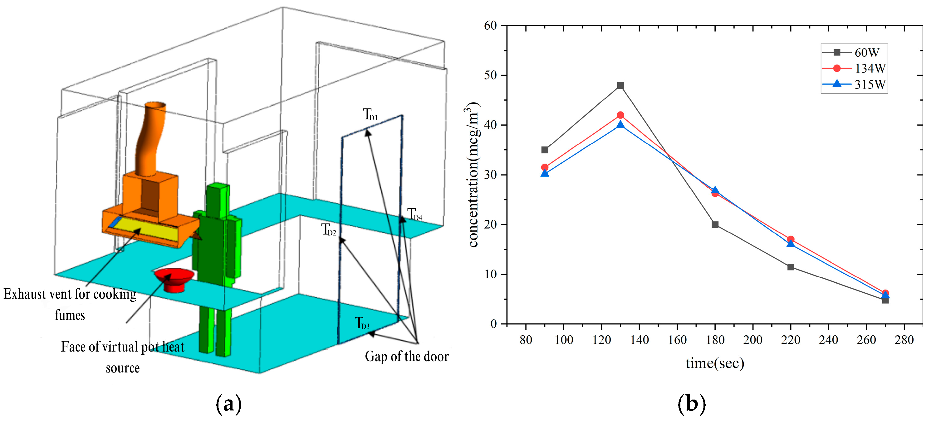
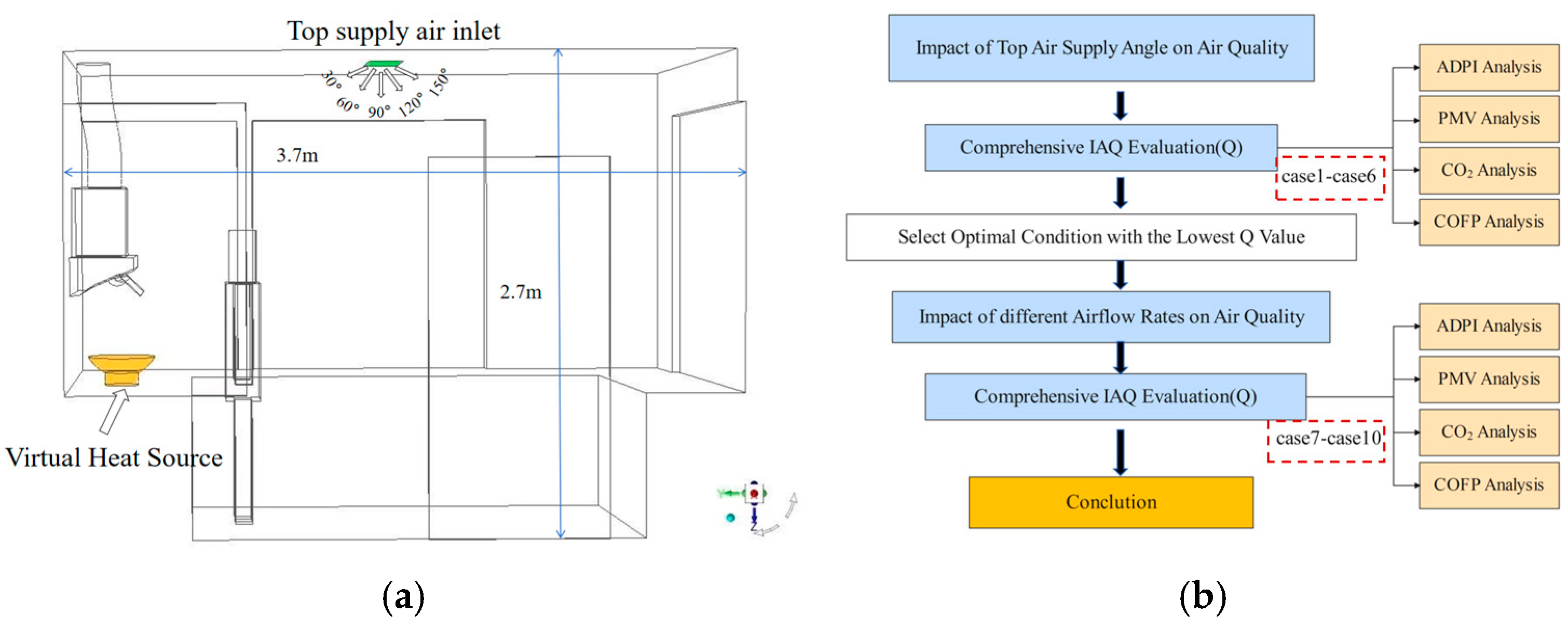
3.2. Geometric Model and Mesh Generation

In this study, the geometric model of the kitchen experimental platform was simplified, and Fluent Meshing was used to generate a polyhedral mesh for the kitchen cooking environment, as shown in Figure 5. To reduce the impact of mesh density on unsteady calculation results, a grid convergence analysis was performed on the mesh model. Three different mesh configurations were considered: 600,000, 1.34 million, and 3.15 million cells. With the top center of the kitchen set as the origin, the temporal variation of COFP concentration at the point (0.2, 0.8, 0.8) above the human body was compared to select a reasonably sized mesh model. The results are shown in Figure 5a, where mesh count serves as the independent variable and COFP concentration as the dependent variable, comparing the time-domain variations of COFP concentration at the same location. The results indicate significant differences in COFP temporal variations between the 600,000-cell and 1.34-million-cell meshes, while the variations between the 1.34-million-cell and 3.15-million-cell meshes were similar. Considering computational efficiency and cost, the 1.34-million-cell mesh was selected for this study, as this configuration adequately meets the computational requirements.

3.3. Physical Model and Boundary Condition Settings

The computational domain boundaries include inlets, outlets, and walls. The door gap is modeled as a pressure outlet set to ambient atmospheric pressure to maintain pressure equilibrium. The range hood exhaust is defined as a negative pressure outlet (−5.6 Pa) to extract cooking fumes. Human surfaces are treated as walls with 16 W/m² heat flux, simulating summer conditions. The pot surface is modeled as a velocity inlet with non-uniform temperature and velocity distributions, where the temperature profile follows a linear distribution between measured center and edge values (Equation (11)).

$$f_l(x,y,z)=-\alpha \left[{\left(x-n\right)}^2+{\left(y-m\right)}^2\right]+\beta , z=\chi$$

(13)

In the equation, $f_l(x,y,z)$ represents the variation of the pot surface temperature as a function of spatial position; $\alpha , \beta$ is the assumed coefficient, set to $3.19\times {10}^{-4}$ based on actual measurements; $n, m, \chi$ are the coordinates of the pot center, with values (0.21 m, 1.56 m, 1.725 m).

However, as the cooking process progresses, the pot surface conditions exhibit highly complex temporal variations in physical parameters including temperature, velocity, and pollutant distribution. Based on experimental measurements, this study employs Fluent embedded ‘Named Expressions’ to mathematically define the spatiotemporal distributions of cooking thermal airflow temperature and velocity, as formulated below:

$$f_t(x,y,z,t)=\left\{\begin{array}{l}{f}_l 0\le t<30 , 200\le t<300\\ {\displaystyle \frac{2}{3}}t+f_l-20 30\le t<45\\ {\displaystyle \frac{8}{135}}t+f_l+{\displaystyle \frac{198}{27}} 45\le t<180\\ {\displaystyle \frac{-9}{10}}t+f_l+180 180\le t<200\end{array}\right.$$

(14)

$$V(t)=\left\{\begin{array}{l}1.5 0\le t<150 \\ {\displaystyle \frac{-3}{40}}t+12.75 30\le t<45\\ 0 45\le t<180\end{array}\right.$$

(15)

where $f(x,y,z,t)$ represents the temperature variation with time t along the vertical axis; $f_l$ represents the temperature variation with respect to the coordinate axis; and $V_{(t)}$ represents the velocity variation with time t.

All other walls are set as adiabatic and no-slip boundaries. The details of boundary conditions and parameter settings for the initial thermal environment are provided in

Table 5. Boundary conditions and parameter settings.

Boundary Name	Boundary Type	Settings
Virtual Heat Source (Pot)	Velocity-inlet	Temperature: Follow Formula (12) $f_t(x,y,z,t)$; Vertical Velocity Profile: 1.5 m/s
Door Gap	Pressure-inlet	Gauge Pressure: 17 Pa Measured Temperatures: TD1–TD4 are 299.3, 297.8, 298.7, 298.4 K
Exhaust Vent	Pressure-outlet	Negative Pressure: 17 Pa Temperature: 283 K
Human Body Surface	Wall (Heat-Flux)	Summer Condition, Surface Heat-Flux: $93{.04 \mathrm{W}/\mathrm{m}}^3$ Roughness Height: 0
Other Surfaces	Wall (No-Slip)	No-Slip Adiabatic Walls Surface Roughness Height: 0 Temperature: 299 K

.

3.4. Numerical Simulation

The cooking process was simulated in the experimental kitchen, as shown in Figure 4. The accuracy of the simulation model was validated by comparing its results with measured temperature and velocity data. The simulation was conducted using a time step of 0.05 s, generating a total of 5400 sets of temperature and velocity data.

Figure 6 presents a comparison of the simulated and experimental results for temperature, velocity, COFP, and CO₂ after applying a 10-s time-averaging process to both datasets. The experimental values closely follow the measured trends, indicating that the simulation model accurately captures airflow perturbations during the cooking process. Overall, deviations remained within 10% for most points at the same locations and time intervals. Despite minor discrepancies, the simulation effectively reproduces the variation patterns of COFP and CO₂ in the kitchen environment, demonstrating its high accuracy and reliability in replicating real-world conditions.

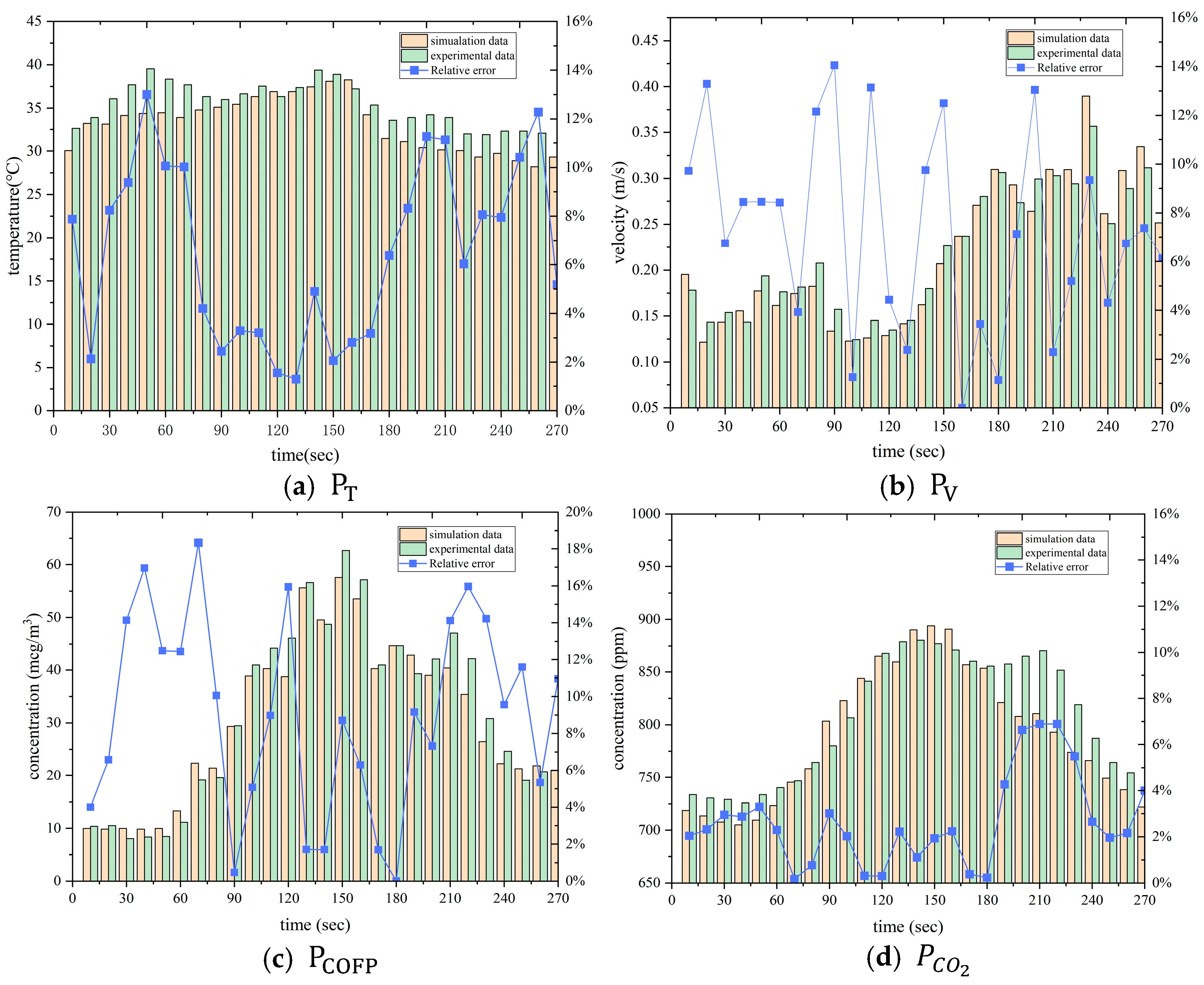
3.5. Quantitative Analysis of Kitchen Air Quality

Several indicators were analyzed in the tested kitchen cooking space to evaluate the impact of airflow temperature and velocity on overall thermal comfort. To quantitatively assess the comfort indicator (ADPI), 36 measurement points were strategically positioned near the subject’s body within the monitoring area. Using ANSYS Fluent 2021R1, temperature and air velocity values were computed at each location, and the ADPI was subsequently calculated through Equations (5) and (6). The locations of the monitoring points are shown in Figure 7. Additionally, this study developed an implementation of the PMV (predicted mean vote) equation in the C programming language. Through the User Defined Functions (UDF) interface in ANSYS Fluent, the custom C program was executed to compute PMV values near the human forehead and mouth. The averaged value of these measurements was derived as the PMV indicator.

To comprehensively analyze CO₂ and COFP concentrations, measurements were taken both in the breathing area and across the entire kitchen. The breathing area refers to the zone where occupants directly inhale air during cooking activities, making its air quality a critical factor for human health. In contrast, the overall concentration reflects the air quality of the entire kitchen space. Focusing solely on the breathing area may overlook pollution in other regions; therefore, this study used the average concentrations from both areas to evaluate CO₂ and COFP levels.

At this stage, the Q value can be calculated by using Equation (12). By incorporating the four key air quality indicators, i.e., ADPI, PMV, CO₂, and COFP, measured at the forehead, breathing point, and across the entire space, this method provides a more precise and comprehensive assessment of indoor air quality. It not only enhances the specificity of air quality evaluation but also offers a more accurate reflection of overall health and comfort in the kitchen environment. The results are presented in

Table 6. Analysis of auxiliary evaluation indicators.

Original Condition	100%-ADPI	Subnasal PMV	Inhalation Area CO2 (ppm)	Entire Kitchen CO2 (ppm)	Inhalation Area COFP (μg/m3)	Entire Kitchen COFP (μg/m3)	Q
	78.41	2.081	736.3	740.9	29.67	28.93	1.634
Ideal Value	100	1	700	700	50	50	1

.

3.6. Experimental Repeatability and Measurement Uncertainty

To assess the repeatability of key indoor air quality (IAQ) indicators, each experimental condition was independently repeated three times.

Table 7. Measurement uncertainties and reproducibility metrics.

Parameter	Instrument	Uncertainty	Reproducibility (CV)
CO2 Concentration	ST8310 recorder	±50 ppm	2.1%
COFP	LH3016 particle counter	±5% of reading	4.3%
Air Velocity	Testo 405i anemometer	±0.03 m/s	1.8%
Temperature	TP9000 data logger	±0.2 °C	0.9%

summarizes the mean values and standard deviations of the primary indicators—including PMV, CO₂, COFP, ADPI, and Q—under the baseline condition (Case 1). The standard deviations were consistently low, indicating high measurement reliability. For example, the standard deviation for PMV at the subnasal position was ±0.09, while CO₂ concentration in the breathing zone varied by only ±18.4 ppm. These deviations represent less than 10% of the mean in all cases, validating the stability of the experimental setup.

4. Optimization Analysis of Kitchen Air Quality

From Table 5, it is evident that during the cooking process, the average PMV value was 2, indicating a perception of warmer ambient temperatures. The average CO₂ concentration exceeded 700 ppm, suggesting unpleasant odors. The average COFP concentration approached 30 µg/m³, indicating that further reduction is necessary. For this reason, it is essential to conduct further studies aimed at optimizing the cooking environment in the kitchen.

4.1. Optimization Strategies

Traditional indoor air supply methods include top supply, displacement ventilation, underfloor air distribution, side supply, and diffuser supply, with the top supply method being the most common and cost-effective. In this study, a rectangular air supply diffuser (0.2 m × 0.4 m) was installed at the center of the kitchen ceiling to improve IAQ during cooking. Initially, the study investigates the impact of different angles of the top air supply (focusing primarily on changes in the longitudinal direction) on IAQ under the same performance conditions (constant air flow rate and supply air temperature). Once the optimal air supply angle is determined, it will be maintained while the air flow rate is adjusted (either reduced or increased by 5% to 10%). For comparison purposes, a setup without upper ventilation was also retained. Figure 8 shows the positioning and optimization of the top air outlet.

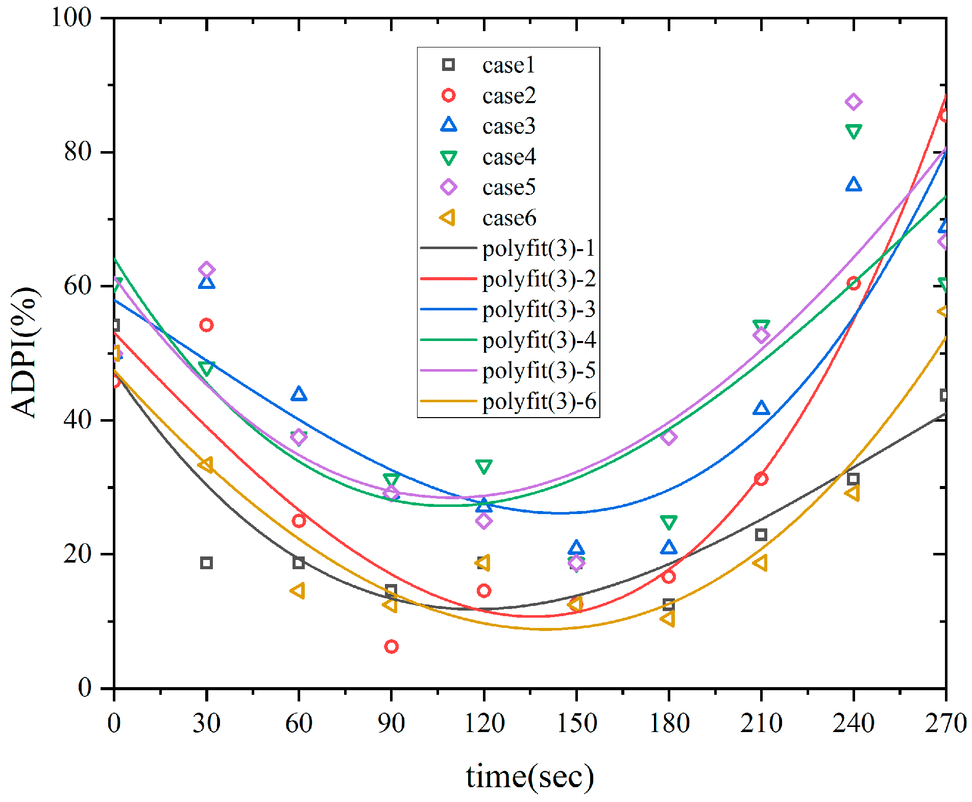
4.2. Simulation Results of Different Working Conditions

In this section, under identical power conditions (constant airflow rate and supply air temperature), five different top air supply angles were systematically designed to analyze their impact on the IAQ. The specific simulation conditions for each angle were detailed in

Table 8. Simulation conditions.

Conditions	Case 1 (Original Condition)	Case 2	Case 3	Case 4	Case 5	Case 6
Air Supply Angle (deg)	0	30	60	90	120	150

Note: The airflow rate is 2.16 m³/min, supply air temperature is 293 K.

.

Figure 9 shows the ADPI values and corresponding fitting curves derived from the analysis of six different operating conditions. The results indicate that the lowest ADPI value for condition 5 was 28.48%, which was 16.64% higher than the original condition’s lowest value of 11.84%, which effectively improved the airflow pattern. Additionally, with the top air supply system remaining active, the ADPI began to increase after 150 s. The optimal performance was observed in condition 5, where the ADPI reached approximately 80% after 270 s. This demonstrates that utilizing an effective top air supply could expedite the removal of hot, polluted air.

Human thermal sensation is a crucial indicator of indoor environmental quality. In this study, the PMV equation was compiled in C language and executed in Fluent via the User Defined Functions (UDF) interface to conduct a quantitative analysis during cooking. The calculation results were shown in Figure 10. The results indicate that the PMV value at the mouth breathing area increased over time, and peaked at 150 s when cooking ceased, influenced by the thermal plume generated during cooking. After cooking, as the effect of the thermal plume diminished, the comfortable airflow produced by the top air supply system significantly enhanced the airflow around the occupant and gradually reduced the PMV value at the mouth breathing area to a comfortable level below 1.5. Among them, it was found that condition 4 had the best performance. The PMV value at the forehead exhibited variability over time due to the combined effects of the cooking heat plume, the upper air supply system, and the heat plume generated by the body’s own heat. In comparison, conditions 4 and 5 provided better thermal comfort.

Figure 11 shows the CO₂ concentration distribution contour at the cross-section of x = 0.21 m and time of 150 s, under different conditions. The results demonstrate that activating the top air supply system could significantly increase the indoor CO₂ removal rate, and air supply angle could directly influence the spatial distribution of CO₂. In conditions 2 to 5, the airflow from the top air supply introduced fresh air to the lower part of the room, reduced CO₂ levels near the occupants and improved IAQ around the face area. At 150 s, the air quality in the room improved from a mildly polluted state to a clean air level, with polluted indoor air been efficiently expelled. According to the contour results, Condition 4 had the best performance.

Figure 12 plots the time-domain fitting curves of the average CO₂ concentration in the breathing area and the average concentration in the room under different conditions. As shown in the figure, the air supply angle in condition 4 effectively reduced the CO₂ concentration in the breathing area during cooking to a maximum of 638 ppm, approximately a 24% reduction (about 220 ppm) from the maximum concentration under the original condition, reaching the clean air standard. In conditions 3 and 5, the CO₂ concentration trends in the breathing area were similar, both remained below 700 ppm, with a maximum concentration approximately 21% lower than that in the original condition. The average concentration trends throughout the room were consistent, primarily influenced by the exhaust from the range hood. The air supply angle in condition 5 effectively enhanced the CO₂ removal efficiency in the room, with a maximum concentration of 730 ppm, which is about 140 ppm, approximately 16% lower than the maximum concentration under the original condition.

Figure 13 shows the spatial distribution of COFP at the time of 150 s under different conditions. The results indicate that COFP ascended to the upper part of the room with the thermal plume generated during cooking and formed a distribution pattern similar to an “air lake”. Vertically, the COFP spatial distribution shows higher concentrations near the top and lower concentrations further down. At 150 s, the top air supply influenced the diffusion behavior of COFP. In condition 2, due to the smaller air supply angle, COFP primarily accumulated near the occupants’ faces, adversely affecting air quality in the breathing area. In conditions 2 to 5, the angles of the air supply were less than 45 degrees relative to the vertical direction, causing some COFP to descend below occupants’ waists. In condition 6, with a supply angle of 150 degrees, although the vertical transport of airflow was not pronounced, it still drove the transport of COFP “attached” to the air flow moved clockwise, reduced the COFP concentration near the occupants and improved overall air quality.

COFP concentration is one of the key indicators for assessing air quality during cooking. Figure 14 presents a time-domain scatter plot of the average COFP concentration in the breathing area and the average concentration throughout the room under different conditions. As shown in the figure, the average COFP concentration in the breathing area is mostly below 50 µg/m³, which is considered within a healthy range. However, due to the complex behaviors of COFP, such as coagulation, transportation, and deposition, the data in the breathing area exhibited significant fluctuations. The trend in the average concentration throughout the room remained relatively consistent, with no significant changes, indicating that the top air supply method had a limited effect on the removal of COFP.

In the present study we employed numerical simulations to calculate time averages of different IAQ under different conditions. The overall assessment index Q was then determined using Equation (6). As shown in

Table 9. Average air quality indicators and evaluation index for different conditions.

Conditions	100%-ADPI	Forehead PMV	Subnasal PMV	Inhalation Area CO2 (ppm)	Entire Kitchen CO2 (ppm)	Inhalation Area COFP (μg/m3)	Entire Kitchen COFP (μg/m3)	Q
Case 1	78.41	2.194	2.081	736.3	740.9	29.67	28.93	1.634
Case 2	64.47	1.888	1.779	659.1	688.0	28.41	27.24	1.414
Case 3	57.99	1.637	1.455	619.3	667.9	25.71	27.87	1.274
Case 4	55.60	1.520	1.335	595.6	651.5	23.73	26.74	1.209
Case 5	53.48	1.490	1.523	623.6	648.5	26.70	26.44	1.226
Case 6	77.19	1.713	1.673	680.9	679.9	30.55	27.29	1.483

, the Q value throughout the kitchen initially increased and then decreased as the angle of the top air supply increased. In condition 4, when the air supply direction is 90°, the IAQ throughout the kitchen was 1.401, which was the optimal configuration, representing a 26.9% reduction in Q value compared to the original condition. If the top air supply angle was either too large or too small, the Q value would exceed 1.5, indicating that the improvement in IAQ is not significant. When compared to the original condition, the Q value decreased only by 7.7% to 14.6%.

After a comprehensive evaluation of all indicators, condition 4 was selected for further optimization. To investigate the impact of airflow rate on kitchen air quality, the original airflow rate settings were adjusted. The simulation cases are shown in

Table 10. Simulation conditions.

Conditions	Case 7	Case 8	Case 9	Case 10
airflow rate (m3/min)	2.052 (−5%)	1.944 (−10%)	2.268 (+5%)	2.376 (+10%)

Note: The airflow rate is 2.16 m³/min, supply air temperature is 293 K.

.

The auxiliary evaluation index for each condition was calculated by integrating the average values of various air quality indicators at different airflow rates, as shown in

Table 11. Average air quality indicators and evaluation index for different conditions.

Conditions	100%-ADPI	Forehead PMV	Subnasal PMV	Inhalation Area CO2 (ppm)	Entire Kitchen CO2 (ppm)	Inhalation Area COFP (μg/m3)	Entire Kitchen COFP (μg/m3)	Q
Case 7	60.61	1.572	1.271	625.1	657.3	25.29	27.62	1.260
Case 8	58.89	1.591	1.390	613.1	650.7	24.43	27.49	1.257
Case 9	52.50	1.465	1.223	594.4	651.1	19.52	26.02	1.152
Case 10	52.22	1.461	1.220	588.0	648.2	22.07	26.37	1.154

. The data indicate that increasing the airflow rate generally improved air quality more effectively than reducing it, when the airflow rate was set at 2.16 m³/min. Among the four conditions, conditions 9 and 10 had the lowest Q, with no significant differences. As the airflow rate increased, the COFP concentration in condition 10 did not decrease but rather increased, indicating a complex trajectory of the COFP over time. The simulation results suggest that higher airflow does not always equate to more effective air quality improvement, and beyond a certain threshold additional airflow yields no significant benefits. Considering energy consumption, condition 9 emerged as the most energy-efficient option for optimal air quality improvement in the kitchen.

4.3. Statistical Significance of Q-Index Improvement

ANOVA with Tukey post hoc testing (α = 0.05) confirmed that Q-index reductions were statistically significant across optimized cases. Cases were grouped by air supply angle (Table 8) and airflow rate (Table 9).The analysis results are shown in

Table 12. ANOVA and Tukey test results for Q-index comparisons.

Comparison Group	F-Statistic	p-Value	Significant Pairs (p < 0.05)	Mean Q ± SD
Air supply angle	F = 37.2	<0.001	Case 4 vs. all others	Case 1: 1.634 ± 0.04 Case 4: 1.209 ± 0.03
Airflow rate	F = 29.8	<0.001	Case 9 vs. 7, 8, 10	Case 9:1.152 ± 0.02 Case10:1.154 ± 0.03

.

For angle optimization, a statistically significant overall effect was observed (F(5,18) = 37.2, p < 0.001), indicating that the tested angles produced substantially different results. Specifically, Case 4 (90°) significantly outperformed Case 1, with a mean difference of 0.425 (95% CI [0.382, 0.468], p < 0.001). Furthermore, Case 4 also showed significantly better performance compared to all other tested angles, with all pairwise comparisons reaching statistical significance (p < 0.01), establishing 90° as the optimal angle.

For airflow rate optimization, a statistically significant overall effect was also found (F(3,12) = 29.8, p < 0.001), confirming that airflow rates influenced the outcome. The optimal airflow rate was identified as Case 9 (2.268 m³/min), which demonstrated a significantly better performance compared to the baseline condition. The mean improvement was 0.482 (95% CI [0.437, 0.527], p < 0.001), confirming Case 9 as the superior airflow rate.

5. Conclusions

5.1. Study Limitations and Future Perspectives

While this study achieves significant IAQ improvement through the Q-index framework, two limitations warrant attention:

(1)

Experiments and simulations focused on an enclosed kitchen without examining interactions with adjacent spaces (e.g., open-plan kitchens integrated with dining/living areas). Future work should investigate multi-zone ventilation synergy and pollutant migration pathways.

(2)

Optimization targeted COFP and CO₂, excluding volatile organic compounds (VOCs) and ultrafine particles (UFPs) prevalent in cooking emissions [1,3]. Expanding monitoring to include formaldehyde, PM_2.5, and VOCs would enhance Q-index comprehensiveness.

(3)

The Q-index methodology shows promise for broader application. Future research should explore its adaptation and validation in diverse indoor environments with high air quality demands and vulnerable populations, such as kitchens in elderly care facilities, schools, hospitals, and daycare centers, where pollutant exposure and thermal comfort are critical public health concerns. Investigating the transferability of the weighting scheme and optimization approach in these contexts could significantly extend the societal impact of this work.

5.2. Key Findings and Sustainability Implications

This study establishes a quantitative framework for optimizing kitchen ventilation through integrated experimental testing and CFD simulation. By developing a calibrated CFD model under real cooking conditions and systematically optimizing air supply parameters, we achieve significant improvements in indoor air quality (IAQ) and thermal comfort, as quantified by a novel comprehensive index Q. The key conclusions are as follows:

5.2.1. Technical Innovations and Performance Enhancement

• A comprehensive evaluation index, Q, was introduced, incorporating four air quality indicators: ADPI, PMV, CO₂, and COFP, to assess overall air quality during cooking.
• Initial unoptimized conditions yielded substandard IAQ: ADPI: 21.59%, PMV: 2.138, CO₂: 738.6 ppm, COFP: 29.3 µg/m³.
• Optimization of top air supply angle (90°) and airflow rate (2.268 m³/min) significantly enhanced performance: ADPI: 57.5%, PMV: 1.334, CO₂: 622.75 ppm, and COFP: 22.77 µg/m³. This represents a 29.5% reduction in air pollution impact versus baseline.
• The statistical rigor of Q-index improvements was established through ANOVA, with effect sizes exceeding measurement uncertainties. The 22–24% reductions in COFP/CO₂ and 29.5% Q-index decline (p < 0.001) confirm that optimization is not attributable to experimental noise. Future studies should expand replicates to address cooking process variability.

5.2.2. Sustainability Implications

• The 29.5% Q-index reduction translates to a 24% decrease in peak CO₂ exposure (from 638 ppm baseline) and 22% lower COFP in breathing zones, mitigating respiratory health risks associated with prolonged exposure to kitchen pollutants [1,2,4]. This improvement in occupant health and well-being directly contributes to Sustainable Development Goal 3 (Good Health and Well-being), specifically target 3.9 aiming to substantially reduce deaths and illnesses from hazardous chemicals and air pollution.
• Optimized airflow (2.268 m³/min) incurs only a 5% energy penalty versus baseline while avoiding the 20–30% over-ventilation typical in conventional systems, demonstrating quantifiable IAQ–energy balance. This reduction in unnecessary energy consumption supports the development of more sustainable and resource-efficient buildings, aligning with Sustainable Development Goal 11 (Sustainable Cities and Communities), particularly target 11.6 on reducing the adverse environmental impact of cities, including air quality.
• The Q-index provides a metrics-driven framework to resolve IAQ–comfort–energy tradeoffs, supporting evidence-based ventilation standards for sustainable urban kitchens. This methodological contribution offers a practical tool for policymakers and building designers striving to meet SDG targets related to health and sustainable urbanization.

This work transcends ventilation optimization by delivering a replicable model for low-carbon, health-protective indoor environments. The Q-index methodology offers industry and policymakers a tool to align building performance with sustainable development objectives.

References

1. Ding, M.; Zhang, S.; Wang, J.; Ye, F.; Chen, Z. Study on spatial and temporal distribution characteristics of the cooking oil fume particulate and carbon dioxide based on CFD and experimental analyses. Atmosphere 2023, 14, 1522. [Google Scholar] [CrossRef]
2. Zhou, B.; Chen, F.; Dong, Z.; Nielsen, P.V. Study on pollution control in residential kitchen based on the push-pull ventilation system. Build. Environ. 2016, 107, 99–112. [Google Scholar] [CrossRef]
3. Pryor, J.T.; Cowley, L.O.; Simonds, S.E. The Physiological Effects of Air Pollution: Particulate Matter, Physiology and Disease. Front. Public Health 2022, 10, 882569. [Google Scholar] [CrossRef]
4. Pini, L.; Giordani, J.; Concoreggi, C.; Zanardini, E.; Pini, A.; Perger, E.; Bargagli, E.; Bona DDi Ciarfaglia, M.; Tantucci, C. Effects of short-term exposure to particulate matter on emergency department admission and hospitalization for asthma exacerbations in Brescia district. J. Asthma Off. J. Assoc. Care Asthma 2022, 59, 1290–1297. [Google Scholar] [CrossRef]
5. Habre, R.; Zhou, H.; PEckel, S.; Enebish, T.; Fruin, S.; Bastain, T.; Rappaport, E.; Gilliland, F. Short-term effects of airport-associated ultrafine particle exposure on lung function and inflammation in adults with asthma. Environ. Int. 2018, 118, 48–59. [Google Scholar] [CrossRef]
6. Posselt, K.P.; Neuberger, M.; Köhler, D. Fine and ultrafine particle exposure during commuting by subway in Vienna. Wien. Klin. Wochenschr. 2019, 131, 374–380. [Google Scholar] [CrossRef]
7. Rittner, R.; Flanagan, E.; Oudin, A.; Malmqvist, E. Health Impacts from Ambient Particle Exposure in Southern Sweden. Int. J. Environ. Res. Public Health 2020, 17, 5064. [Google Scholar] [CrossRef]
8. Delgado-Saborit, J.M.; Aquilina, N.J.; Meddings, C.; Baker, S.; Harrison, R.M. Relationship of personal exposure to volatile organic compounds to home, work and fixed site outdoor concentrations. Sci. Total Environ. 2011, 409, 78–88. [Google Scholar] [CrossRef] [PubMed]
9. Klepeis, N.E.; Nelson, W.C.; Ott, W.R.; Robinson, J.P.; Tsang, A.M.; Switzer, P.; Behar, J.V.; Hern, W.H.; Engelmann, S.C. The National Human Activity Pattern Survey (NHAPS): A resource for assessing exposure to environmental pollutants. J. Expo. Anal. Environ. Epidemiol. 2001, 11, 31–52. [Google Scholar] [CrossRef]
10. Fanger, P.O. Thermal Comfort Analysis and Applications in Environment Engineering. Environ. Eng. 1972, 45, 244. [Google Scholar]
11. Toftum JJorgensen, A.S.; Fanger, P.O. Upper limits for indoor air humidity to avoid uncomfortably humid skin. Energy Build. 1998, 28, 1–13. [Google Scholar] [CrossRef]
12. Kuchen, E.; Fisch, M. Spot Monitoring: Thermal comfort evaluation in 25 office buildings in winter. Build. Environ. 2008, 44, 839–847. [Google Scholar] [CrossRef]
13. Buratti, C.; Mariani, R.; Moretti, E. Mean age of air in a naturally ventilated office: Experimental data and simulations. Energy Build. 2011, 43, 2021–2027. [Google Scholar] [CrossRef]
14. Chen, Z.; Xin, J.; Liu, P. Air quality and thermal comfort analysis of kitchen environment with CFD simulation and experimental calibration. Build. Environ. 2020, 172, 106691. [Google Scholar] [CrossRef]
15. Song, J. Research on the Impact of Ventilation and Air Conditioning System Forms on Indoor Air Quality. Build. Therm. Vent. Air Cond. 2021, 40, 89–93. [Google Scholar]
16. Fan, L. Research on the Impact of Residential Ventilation Systems on Indoor Air Quality; Beijing University of Civil Engineering and Architecture: Beijing, China, 2021. [Google Scholar]
17. Lin, J.; Zhou, T.; Qiu, Y. Numerical Simulation of Thermal Comfort Suitability of Cabin Under Different Air Conditioning Working Conditions. Fluid Dyn. Gas Dyn. 2022, 46, 86–93. [Google Scholar]
18. Wang, F.; Lin, X.; Hou, Y. Impact of Radiation Air Supply Methods on Cabin Thermal Comfort of Ships. Ship Eng. 2022, 44, 69–75. [Google Scholar] [CrossRef]
19. Zhang, C.Q.; Yang, F.; Xia, Y.F.; He, L.J.; Yu, Y.L.; Zeng, L.J.; Cao, C.S.; Gao, J. Make-up air optimization and demand exhaust rate of commercial kitchens under multiple cookers operation. J. Build. Eng. 2024, 89, 109274. [Google Scholar] [CrossRef]
20. Zhang, S.Y.; Huang, X.Y.; Li, A.; Yu, B.S.; Jiang, Y.; Peng, L.; Chen, Z.L. Improving kitchen thermal comfort in summer based on optimization of airflow distribution. J. Build. Eng. 2024, 96, 110614. [Google Scholar] [CrossRef]
21. Li, J.Q.; Liu, A.Q.; Yu, L.; Meng, C.; Ma, Y.C.; Dong, J.K. Influence and optimal operating parameters of slit make-up air system on low-energy kitchen environment. J. Build. Eng. 2024, 94, 110016. [Google Scholar] [CrossRef]
22. Song, Y.L.; Chen, X.; Zhang, Z.; Cao, S.; Du, T.; Guo, H.F. Studies on the control of kitchen pollutants by exhaust hood with air-filled slots. J. Build. Eng. 2022, 48, 103891. [Google Scholar] [CrossRef]
23. Liu, Y.; Li, C.; Ma, H.Q.; Luo, X.M. Performance of local supply-exhaust ventilation around stove with numerical simulation in a residential kitchen. J. Build. Eng. 2024, 87, 109078. [Google Scholar] [CrossRef]
24. Xie, W.H.; Gao, J.; Lv, L.P.; Hou, Y.M.; Cao, C.S.; Zeng, L.G.; Xia, Y.F. Parametrized design for the integration of range hood and air cleaner in the kitchen. J. Build. Eng. 2021, 43, 102878. [Google Scholar] [CrossRef]
25. Wu, X.; Cui, W.Z.; Wang, Y.X.; Xiang, W.F. Human thermal comfort in kitchen with different ventilation modes based on a coupled CFD and thermoregulation model. J. Build. Eng. 2024, 94, 110000. [Google Scholar] [CrossRef]
26. Lin, J.; Wu, J.; Lian, M. Optimization of Cabin Thermal Comfort Based on ADPI and Blowing Sensation Index. Fluid Dyn. Gas Dyn. 2018, 46, 40–45. [Google Scholar]
27. Li, J.; Wu, X.; Yang, R. Analysis of Improvement Measures for the Concentration of Harmful Substances in Ships. China Water Transp. 2013, 13, 204–205. [Google Scholar]
28. Zhang, S.; Li, B.; Li, A. Research on Constant-Flow Water-Saving Device Based on Dynamic Mesh Transient Flow Field Analysis. Water 2024, 16, 2427. [Google Scholar] [CrossRef]
29. JCGM 100:2008; Evaluation of Measurement Data—Guide to the Expression of Uncertainty in Measurement. BIPM: Sèvres, France, 2008.
Figure 1. Kitchen Test Scenarios. (a) Monitoring point for pollutants and airflow pattern; (b) 3D layout of monitoring points.
Applsci 15 06755 g001
Figure 2. Testing instruments used for various parameters in kitchen experiments. (a) Handheld particle counter LH3016; (b) TOPRIE TP9000 multi-channel data recording; (c) ST8310A CO2 recorder; (d) Testo 405i Thermal Anemometer.
Applsci 15 06755 g002
Figure 3. A photograph of kitchen experiments.
Applsci 15 06755 g003
Figure 4. Timeline of cooking test.
Applsci 15 06755 g004
Figure 5. Schematic diagram of the kitchen environment geometric model and convergence analysis. (a) Kitchen geometric model; (b) Convergence analysis curve graph of the grid.
Applsci 15 06755 g005
Figure 6. Time-domain comparison curves of simulation and experimental values at different monitoring points.
Applsci 15 06755 g006
Figure 7. ADPI monitoring points near occupant. (a) Front view of the monitoring points. (b) Top view of the monitoring occupant.
Applsci 15 06755 g007
Figure 8. Schematic diagram of top air supply outlet and optimization flowchart. (a) Schematic Diagram of Top Air Supply Outlet; (b) Optimization Flowchart.
Applsci 15 06755 g008
Figure 9. Fitted scatter plot of ADPI over time for different conditions.
Applsci 15 06755 g009
Figure 10. Fitted plot of PMV over time for different conditions.
Applsci 15 06755 g010
Figure 11. CO2 concentration contours at cross-section x = 0.21 m and time 150 s under different conditions.
Applsci 15 06755 g011
Figure 12. Fitted scatter plot of CO2 variation over time for different conditions. (a) Average concentration at breathing area of occupant; (b) Indoor average concentration.
Applsci 15 06755 g012
Figure 13. COFP concentration contours at x = 0.21 m cross-section at 150 s for different conditions.
Applsci 15 06755 g013
Figure 14. Scatter plot of COFP over time for different operating conditions. (a) Average concentration at breathing area of occupant; (b) Indoor average concentration.
Applsci 15 06755 g014