Evaluating the Efficiency of Nature-Inspired Algorithms for Finite Element Optimization in the ANSYS Environment

Abstract

Nature-inspired metaheuristics have proven effective for addressing complex structural optimization challenges where traditional deterministic or gradient-based methods often fall short. This study investigates the feasibility and benefits of embedding three prominent metaheuristic algorithms, the Genetic Algorithm (GA), the Firefly Algorithm (FA), and the Group Search Optimizer (GSO) embedded into the ANSYS Parametric Design Language (APDL). The performance of each optimizer was assessed in three case studies. The first two are spatial truss structures, one comprising 22 bars and the other 25 bars, commonly used in structural optimization research. The third is a planar 15-bar truss in which member sizing and internal topology were simultaneously refined using a Discrete Topology (DT) variable method. For both the FA and the GSO, enhanced ranger-movement strategies were implemented to improve exploration–exploitation balance. Comparative analyses were conducted to assess convergence behavior, solution quality, and computational efficiency across the different metaheuristics. The results underscore the practical advantages of a fully integrated APDL approach, highlighting improvements in execution speed, workflow automation, and overall robustness. This work not only provides a comprehensive performance comparison of GA, FA, and GSO in structural optimization tasks, but it can also be considered a novelty in employing native APDL routines for metaheuristic-based finite element analysis.

1. Introduction

Optimization methods are essential in structural engineering, particularly for rapidly evaluating and analyzing complex systems during preliminary design. In damage identification tasks, for example, accurately estimating the degraded stiffness or cross-sectional areas of elements within large truss structures can be formulated as a minimization problem: measured displacements and strains serve as inputs to an objective function, and an optimizer seeks the parameter values that best reconcile model predictions with observations. In [1], a partial-model-based strategy for long-span steel truss bridges leverages this paradigm by constructing localized stiffness matrices around suspected damage zones, thereby reducing the dimensionality of the global problem. Displacement and strain measurements drive the objective function, which is minimized through two local-search optimizers: the derivative-free Nelder–Mead simplex method [2] and a derivative-based quasi-Newton algorithm. Applied to several regions of a truss bridge, this approach successfully identifies and quantifies damage, with the quasi-Newton solver demonstrating rapid convergence compared to the Nelder–Mead routine. While local optimizers like Nelder–Mead and quasi-Newton excel at fine-tuning solutions in relatively smooth, convex landscapes, structural applications often involve highly nonlinear, multimodal response surfaces, particularly when topology, material heterogeneity, or discrete design variables come into play. In such cases, metaheuristic algorithms inspired by natural phenomena have emerged as powerful tools for addressing complex optimization tasks, particularly when traditional deterministic or gradient-based methods prove insufficient [3]. These approaches, inspired by biological evolution and collective behaviors observed in nature, have yielded notable successes across a variety of engineering and scientific disciplines. Prominent among these are the Genetic Algorithm (GA) [4,5,6,7,8,9], the Firefly Algorithm (FA) [10,11,12,13,14], and the Group Search Optimizer (GSO) [15,16,17,18,19], each distinguished by a unique strategy for exploring the search space.

The Genetic Algorithm, whose foundational concepts and schema theory were introduced by Holland in 1975 [4], represents one of the earliest and most thoroughly studied evolutionary metaheuristics. GA maintains a population of candidate solutions that evolve through iterative application of selection, crossover, and mutation operators. Individuals are evaluated by a fitness function, with higher fitness solutions having a greater reproducing probability, thereby transmitting their advantageous traits to the next generation. Crossover promotes the recombination of promising genetic material, while mutation injects controlled randomness to preserve diversity and mitigate premature convergence. Since its inception, GA has been applied extensively within structural optimization contexts: continuum and plate topology design [5], composite-material configuration [6,7], shape optimization of solid components [8], and sizing optimization in truss and frame systems [9], among others. For example, in [5], the authors proposed a graphical encoding scheme for continuum topology, together with customized crossover and mutation operators that preserve key geometric features. In [6], an adaptive-operator GA incorporating an “elite comparison” mechanism optimizes fiber orientations in composite laminates, achieving accelerated convergence. A multi-objective GA for stacking-sequence design in lightweight composites is presented in [7], where mechanical constraints and objectives are embedded into the initialization and selection processes. In reference [8], the efficacy of the GA methodology is illustrated through two case studies in which material is selectively removed or added to achieve the final optimal shape of the component. Finally, Ref. [9] introduces a hybrid method that couples a classical GA with a probabilistic local search, effectively minimizing the weight of truss structures.

The Firefly Algorithm was formalized by Xin-She Yang in 2010 [10], drawing inspiration from fireflies’ bioluminescent signaling. In FA, each firefly symbolizes a candidate solution, with its “brightness” proportional to the objective function value. Fireflies of lower brightness are drawn toward those of higher brightness (often referred to as the “queen” firefly), traversing the search space according to attractive forces that diminish with distance. Key parameters govern light-attenuation rates, thereby regulating convergence speed and the balance between global exploration and local exploitation. Owing to its capacity to explore complex, multimodal landscapes, FA has demonstrated competitive performance on a variety of optimization challenges [11,12,13,14].

The Group Search Optimizer, introduced by He et al. in 2006 [15], is inspired by the foraging strategies observed in animal groups. In structural engineering, Lijuan Li and Feng Liu [16] extended GSO to multi-objective structural design, balancing criteria such as weight, stiffness, and natural frequency. GSO categorizes individuals into three roles (producers, scroungers, and rangers) to manage exploration and exploitation. Producers execute directed searches based on angular and distance criteria to locate high-quality solutions. Scroungers follow successful producers, exploiting discovered optima, while rangers perform random walks that promote diversity. This social-dynamic framework ensures a robust trade-off between intensification (exploitation) and diversification, facilitating effective global exploration. Accordingly, GSO has exhibited strong performance in civil and mechanical engineering structural optimization problems [17,18,19]. Although GA, FA, and GSO differ in their biological inspirations and algorithmic details, their success hinges upon careful parameter calibration and a dynamic balance between the exploration and exploitation phases.

In recent years, numerical modeling has become a key tool for the analysis and optimization of complex systems. In particular, ANSYS [20] has established itself as a versatile and robust simulation environment, capable of tackling structural mechanics, fluid dynamics, or heat transfer problems across a wide range of application domains. The present work examines the integration of these three nature-inspired metaheuristics within ANSYS 2020 R2 APDL for structural optimization. Embedding the algorithms directly in APDL routines obviates the need for external coupling through Python (3.13.0)-based interfaces (e.g., PyANSYS (release 0.69) [21]), ensuring seamless compatibility with ANSYS solvers and reducing communication overhead. This native implementation enhances computational efficiency, particularly in high-fidelity simulations with large finite element models, where the communication and the data transfer can substantially affect overall performance. Furthermore, APDL-based integration affords tighter control over the simulation workflow and enables resource-efficient automation. The primary objective of this work is to provide a comparative analysis of GA, FA, and GSO when applied to structural optimization tasks while assessing the feasibility and benefits of a fully APDL-embedded solution. In addition, novel “ranger-movement” strategies are introduced for both FA and GSO. Instead of fixed, homogeneous displacement rules, each firefly or ranger may select among four distinct motion modes, thereby dynamically adjusting the balance between global exploration and local exploitation. This adaptive mechanism enables the algorithms to escape local minima and concentrate search effort in promising regions, yielding more robust and efficient convergence behaviors across multiple case studies.

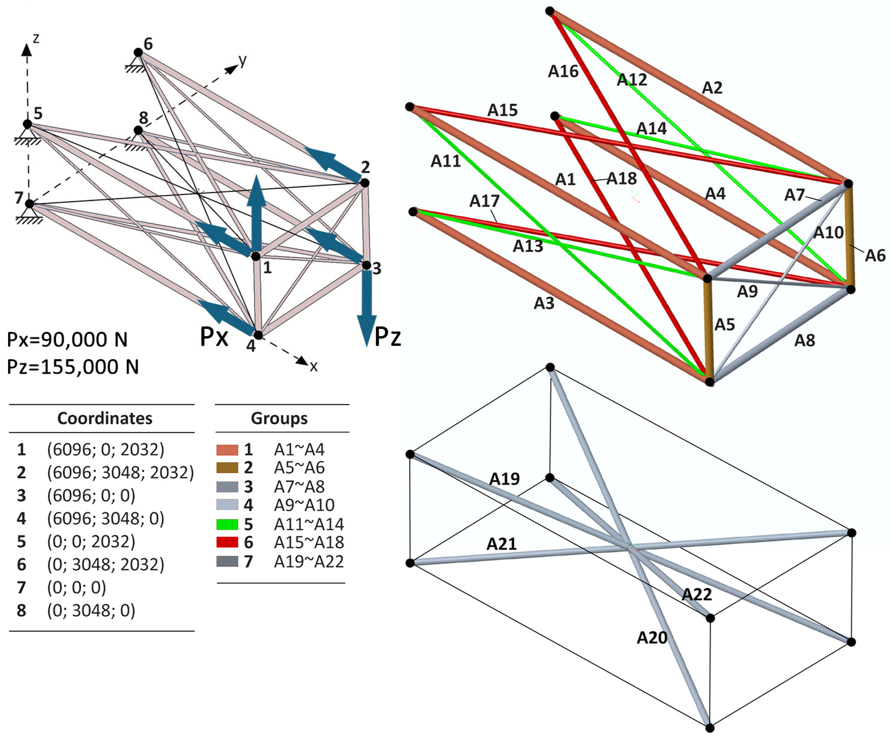
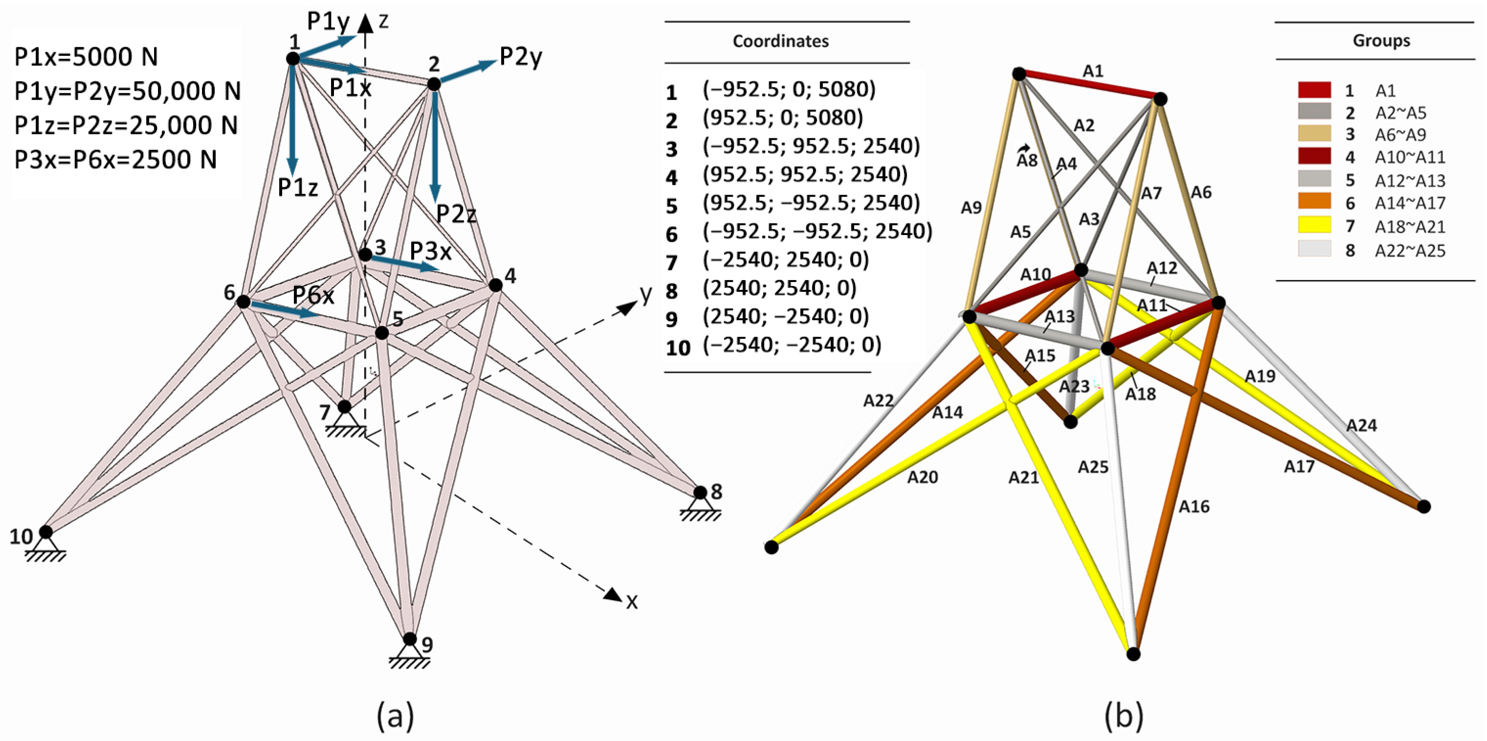
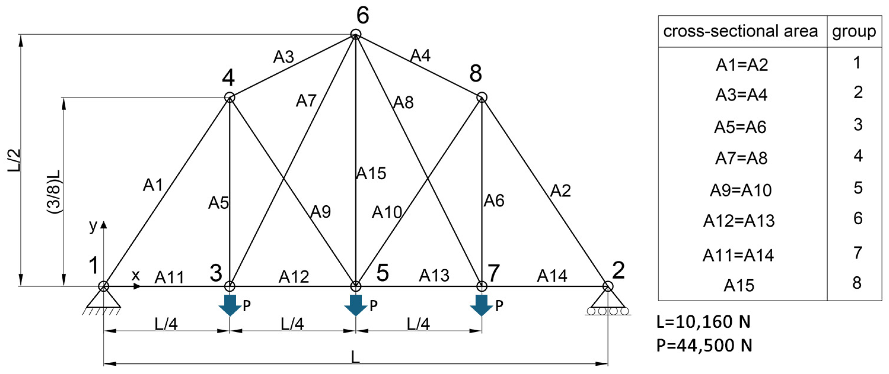
To validate the proposed framework, the algorithms are applied to benchmark spatial truss structures under prescribed loads. Case A considers a 22-bar truss and case B a 25-bar truss, both widely recognized in the literature as standard test cases for structural optimization [17]. Case C employs a Discrete Topology (DT) Variable Method on a 15-rod two-dimensional structure to further improve optimization efficiency. By discretizing topology variables into a finite set of viability-checked configurations, the DT approach reduces the solution space, thereby lowering computational complexity and accelerating convergence. Each metaheuristic (GA, FA, and GSO) is executed in these three cases, with resulting solutions compared in terms of convergence behavior, solution quality, and computational effort.

2. Case Studies

In this study, three distinct case studies (A, B, and C) are analyzed to evaluate the performance of the implemented optimization algorithms [16]. In the following sections, the term design variables (DVs) includes all the continuous parameters optimized by the algorithms, such as outer diameters, thicknesses, and nodal coordinates. In addition, a special variable named discrete topological variable (DT) is introduced (case C study). Although treated as a continuous DV in the range [0, 1], the DT is internally mapped to a discrete set of five predefined structural configurations, enabling topology optimization.

2.1. Case A Study

In case A, a three-dimensional truss structure composed of 22 tubular rods organized into seven groups is examined (Figure 1). Each group is defined by a specific cross-sectional area (Ai, where 1 ≤ i ≤ 22), resulting in a parameterization that includes 14 design variables (7 outer diameters ranging from OD_min = 30 mm to OD_max = 200 mm and 7 thicknesses ranging from TK_min = 0.1 mm to TK_max = 14 mm). A configuration is considered feasible if it satisfies the prescribed limits on three state variables (SVi, where 1 ≤ i ≤ 3):

• SV1: Minimum allowable cross-sectional area A_min = 64.5 mm²;
• SV2: Stress limits of the members (see

  Table 1. Tensile and compressive stress limits for the case A and case B studies.

  Group	Case A		Case B
  	Compressive Stress Limits [MPa]	Tensile Stress Limits [MPa]	Compressive Stress Limits [MPa]	Tensile Stress Limits [MPa]
  1	165	248	242	275
  2	207	248	80	275
  3	193	248	120	275
  4	179	248	242	275
  5	152	248	242	275
  6	138	248	46	275
  7	124	248	48	275
  8	-	-	80	275

  );
• SV3: Displacement limits of each node DL = ±50 mm.

In all case studies, the Objective Function Value (OFV), defined as the total weight of the structure, is minimized.

2.2. Case B Study

The second case study (case B) involves a more complex truss configuration characterized by 16 design variables (8 outer diameters ranging from OD_min = 30 mm to OD_max = 200 mm and 8 thicknesses ranging from TK_min = 0.1 mm to TK_max = 14 mm) with cross-sectional area (Ai, where 1 ≤ i ≤ 25) organized into eight groups (Figure 2), while maintaining the same three state variables (see Table 1 for tensile and compressive stress limits) and objective function value for feasibility. This case allows for a deeper investigation into the interplay between increased design variable complexity and optimization performance under more stringent constraints.

2.3. Case C Study

The final case study (case C) examines a two-dimensional truss structure composed of 15 rods, organized into eight groups according to their cross-sectional properties (see Figure 3). Although the configuration may appear impractical from an engineering design standpoint, it is widely adopted in the literature as a benchmark model for evaluating the performance and robustness of structural optimization algorithms.

In this case, three state variables are defined:

• SV1: Minimum allowable cross-sectional area A_min = 64.5 mm²;
• SV2: Stress limits of all the members SL = ±172.45 MPa;
• SV3: Displacement limits of each node DL = ±20 mm.

This configuration exhibits increased complexity, with a total of 22 design variables. Specifically, 16 of these correspond to sizing parameters: 8 outer diameters (ranging from OD_min = 80 mm to OD_max = 300 mm) and 8 thicknesses (ranging from TK_min = 10 mm to TK_max = 39 mm). Five additional variables determine the positions of nodes 3, 4, 6, 7, and 8 (see

Table 2. Node coordinates of the case C structure.

Node	x-Coordinate	y-Coordinate
1	−L/2	0
2	L/2	0
3	−L/8 ≤ x ≤ −(3/8)L	0
4	−L/8 ≤ x ≤ −(3/8)L	L/16 ≤ y ≤ (3/8)L
5	0	0
6	0	L/8 ≤ y ≤ L/2
7	L/8 ≤ x ≤ (3/8)L	0
8	L/8 ≤ x ≤ (3/8)L	L/16 ≤ y ≤ (3/8)L

, where L = 10,160 mm, and Figure 3).

Furthermore, five distinct configurations are evaluated to explore various internal topologies (Figure 4).

In particular, in each iteration of the algorithm, the discrete topological variable DT (see

Table 3. Topology selection for the case C structure.

Range Value of the Topological Variable DT	Configuration of Figure 4
0 ≤ DT < 0.2	type (a)
0.2 ≤ DT < 0.4	type (b)
0.4 ≤ DT < 0.6	type (c)
0.6 ≤ DT < 0.8	type (d)
0.8 ≤ DT ≤ 1.0	type (e)

) is determined, yielding a specific rod configuration, as shown in Figure 4.

This comprehensive parameterization not only presents a challenging optimization problem but also facilitates the investigation of topology optimization via a discrete topology variable method.

3. Design Variables and Optimal Solution Array Structure

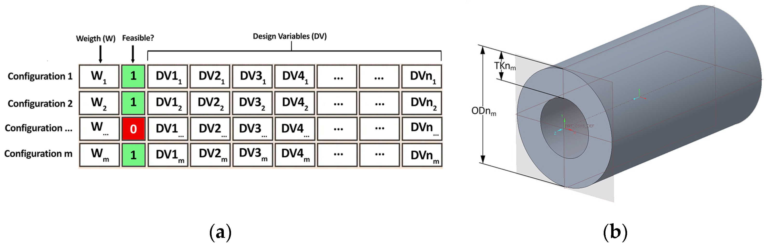
In this study, it is essential to define the array of the Design Variables (DVs, see Figure 5a).

In detail, each structure configuration modeled in ANSYS is defined by specific design variables, i.e., dimensionless parameters ranging from 0 to 1. From these parameters, the corresponding dimensional quantities (for example, the outer diameter of the rods or the wall thickness, see Figure 5b) can be calculated via appropriate mathematical formulations. For example, the outer diameter of the rods is obtained from Equation (1), where the subscript “n” identifies the n-th design variable, and the subscript “m” identifies the m-th configuration:

ODn_m = (1 − DVn_m) · OD_min + DVn_m · OD_max

(1)

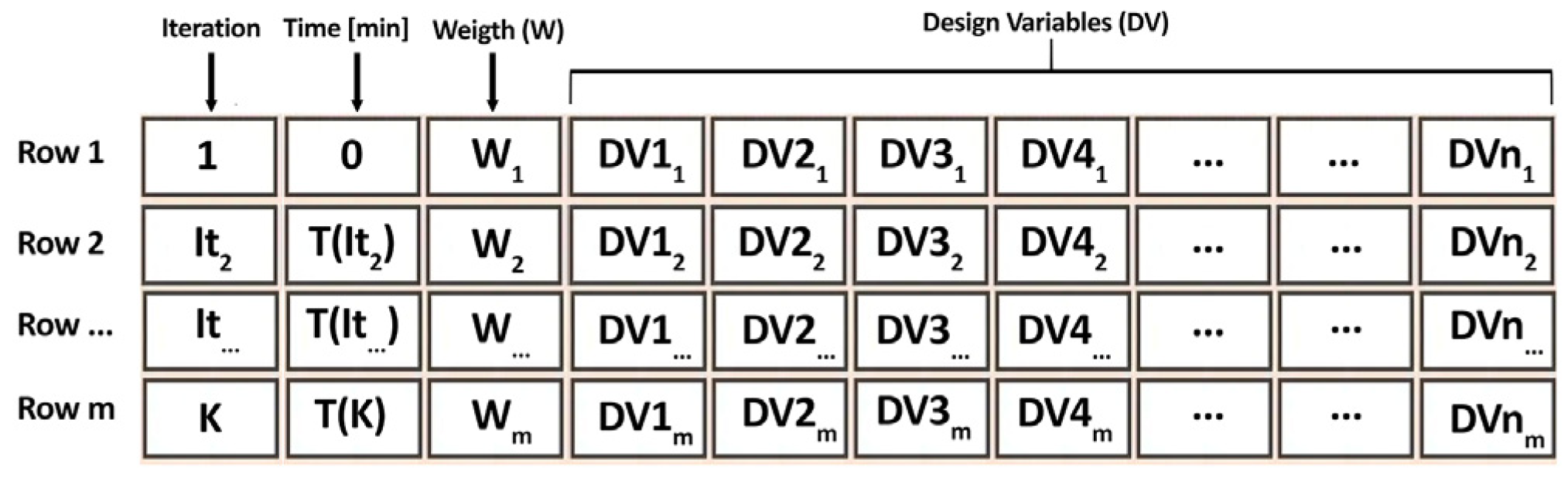
To facilitate the optimization process, the first column of the dataset stores the structural weight, while the second column contains a [0–1] feasibility parameter. This parameter indicates whether a given configuration meets all required state variables. If it is zero, that configuration is excluded from further optimization cycles. Figure 6 illustrates the structure of the optimal solution array. In particular, whenever the system identifies an improved configuration, the software updates a table in which column 1 shows the iteration number, column 2 records the timestamp when a new improved solution is found, and column 3 shows the corresponding objective function value (weight W). Therefore, after the algorithm determines a new optimal value, it appends a new row to this table, ensuring full traceability and supporting subsequent numerical analyses.

4. Nature-Inspired Algorithms

The optimizer is implemented as a comprehensive suite of native ANSYS macros [20] and is therefore fully embedded within the ANSYS APDL environment. This close integration means that no external executables or wrappers are required to drive the optimization loop; instead, all logic resides within ANSYS itself. Communication between the optimization routines and the finite-element solver is handled entirely via ANSYS parameter objects (for passing design variables, convergence thresholds, and constraints) and result objects (for retrieving objective function values and constraint data). In practice, this means that in each generation, the primary control script (the “master macro”) sequentially invokes the following:

(1) Parameter Initialization (file parameters.mac): Here, the number of design variables, their initial bounds, convergence criteria, and any user-defined constraints are established. Because this is coded as an ANSYS macro, these settings are loaded directly into the APDL parameter table, eliminating the need for separate data files or manual transfers.

(2) Geometry and Mesh Generation (geometry.mac): Once the parameters are in place, the master macro calls geometry.mac. This routine constructs or updates the CAD/finite-element model entirely within ANSYS. Any change in design variables, such as dimensional values, material property assignments, mesh controls, loads, or boundary conditions, propagates immediately to the model because geometry.mac interfaces directly with ANSYS’s geometry kernel and meshing routines. After the geometric model is defined, the same geometry.mac applies mesh controls, defines element type, assigns material properties, and establishes loads and boundary conditions. The ANSYS solver is then launched in the same session. Once the analysis completes, the resulting data (e.g., nodal displacements or stress distributions) are stored in ANSYS result objects.

(3) Metaheuristic Algorithm (FA.mac, GA.mac, or GSO.mac): Depending on the chosen metaheuristic, the master macro transfers control to one of three algorithm-specific macros: FA.mac (for Firefly Algorithm), GA.mac (for Genetic Algorithm), and GSO.mac (for Group Search Optimization). Each of these macros follows a similar overarching procedure:

• Fitness Evaluation: Using *GET commands, the macro determines objective function values (total weight) and constraint metrics (such as maximum stress or displacement) directly from the result objects generated by the solver.
• Population/Agent Update: Based on the retrieved values, the macro applies the respective metaheuristic’s update rules to generate new candidate designs (e.g., firefly movement equations in FA, crossover/mutation in GA, or member movement in GSO).
• Parameter Overwrite: The newly computed design variables are written back into the ANSYS parameter table, ready for the next call to geometry.mac.

Because all of these routines are native ANSYS macros, each generation’s new designs are fed back into the master routine without ever leaving the APDL environment. This coupling (geometry → mesh/solver → result extraction → design update) continues iteratively until the convergence criteria defined in parameters.mac are satisfied. The result is an in-memory optimization loop in which both the optimizer and the solver coexist in a single ANSYS session. In the following sections, t denotes the current iteration index, while N_lim refers to the maximum number of iterations allowed for each optimization run.

4.1. Genetic Algorithm

As already mentioned, the genetic algorithm is integrated into ANSYS APDL via a custom set of routines. The implementation follows the standard steps of a GA: initialization of an initial population, fitness evaluation, selection, crossover, mutation, and reinsertion of the best solutions. Two main termination criteria are adopted: a maximum allowed CPU time and a maximum number of consecutive iterations without improvement, ensuring the process converges in a controlled manner. Figure 7 provides a graphical overview of the workflow for the first phase of the optimization cycle.

First, a fixed number of chromosomes is randomly generated, each encoding a feasible set of dimensionless design variables, as explained in paragraph 2, which will allow the determination of the dimensional variables of the examined structures, e.g., external diameters and thicknesses. These chromosomes are evaluated according to a specific objective function to be minimized and calculated using the ANSYS solver, here, the weight W of the structure. 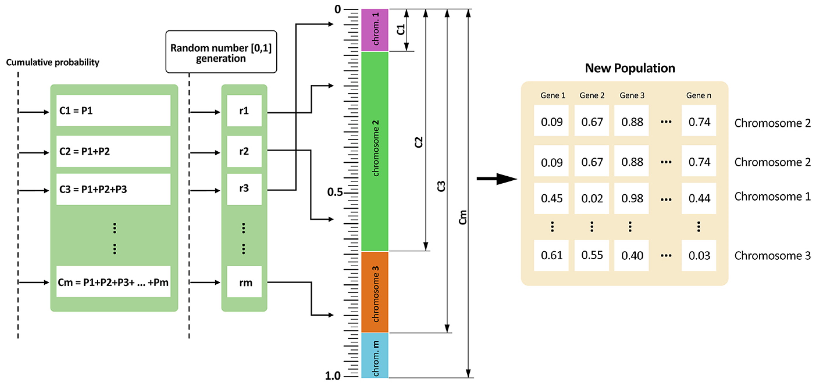Subsequently, the fitness function Fc of each chromosome is calculated as Fc = 1/1 + W. This formulation ensures that better (i.e., lighter) solutions have higher fitness values. Each probability of the chromosomes being chosen is proportional to its fitness, which helps ensure that fitter solutions have higher chances of being passed on to subsequent generations. In order to select which chromosomes participate in the creation of offspring, a roulette-wheel method is used (see Figure 8). The algorithm also retains the globally best solution found so far, preventing the loss of superior designs due to random fluctuations.

Crossover is performed on the selected chromosomes, either at one or two split points (or randomly chosen), to produce new candidate solutions that blend features from the parent chromosomes. A user-defined crossover probability controls how often this genetic exchange occurs. Subsequently, in the mutation phase, a fraction of the newly created genes is altered at random based on a specified mutation rate, thus promoting diversity in the population and reducing the risk of premature convergence.

The reinsertion step merges the newly generated offspring with the existing population and then re-sorts the extended set of solutions by fitness. To limit the overall population size, only a predefined number of the best-performing chromosomes are retained, effectively discarding inferior designs. This “fitness-based reinsertion” technique balances the need to explore new regions of the design space with the requirement to preserve promising individuals.

At each generation, the algorithm updates the global best solution and logs the iteration, time, and objective function value. The process continues until either the maximum CPU time is reached or the improvement counter exceeds its threshold, indicating that no better solution has been identified for a prescribed number of consecutive cycles. Upon termination, the best chromosome is reported as the final solution, alongside the required computational time.

4.2. Firefly Algorithm

As highlighted in the introduction, the Firefly Algorithm draws its inspiration from the social flashing behavior of fireflies and the way they communicate through bioluminescence. In FA, each firefly represents a candidate solution in the search space, and its “brightness” corresponds to the quality of that solution. When two fireflies encounter one another, the less bright individual moves toward the brighter one, often referred to as the “queen” firefly, so long as the brighter firefly lies within a certain attraction range.

This attraction is governed by an inverse-square relationship: as the distance between two fireflies increases, the perceived light intensity falls off in proportion to the square of that distance. In practice, we model this using an attractiveness function β (Equation (2)) which attains its maximum value β₀ when the distance is zero and decays according to a user-defined light-absorption coefficient γ. As shown in [12], β₀ is commonly set to 1.

$$\beta ={\beta }_0{e}^{-\gamma d^2}$$

(2)

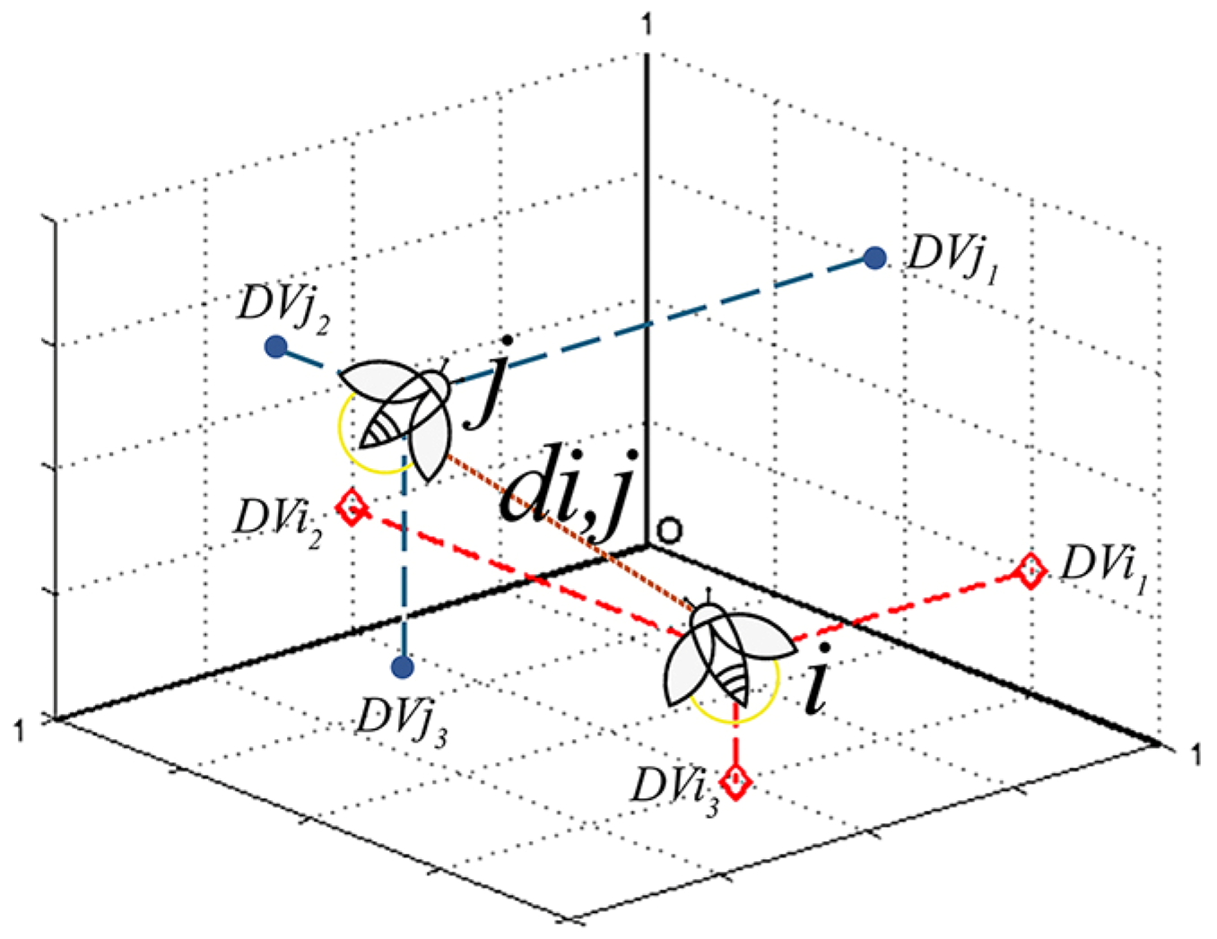
In Equation (2), d denotes the Euclidean distance, which is given by Equation (3). Figure 9 shows a schematic representation of this distance in three-dimensional space.

$$d_{ij}=\sqrt{({DVi}_1-{DVj}_1{)}^2+({DVi}_2-{DVj}_2{)}^2+\cdots +({DVi}_m-{DVj}_m{)}^2}$$

(3)

The parameter γ has a relevant impact on the analysis convergence rate: small values encourage broader exploration by allowing fireflies to influence one another over longer distances, while larger values concentrate the search locally. In most engineering applications, γ is tuned between 0.01 and 10. In the study, we selected γ = 1 [10,12] to strike a balance between exploration and exploitation.

The movement of each firefly combines deterministic attraction with a stochastic component. After computing the Euclidean distance to any brighter neighbor, a firefly updates its position by moving toward that neighbor proportional to its attractiveness (see Equation (4)), then adds a random perturbation (parameter α⋅ε_i) to encourage local exploration around its new location. Specifically, the position update from the t iteration to the next is given by Equation (4), where α = 0.2 [10,12] and ε_i is a random number in the range [−1, 1].

$${DVi}^{t+1}={DVi}^t+{\beta }_0{e}^{-\gamma d_{ij}^2}·\left({DVj}^t-{DVi}^t\right)+\alpha \cdot {\epsilon }_i$$

(4)

Unlike existing literature, our implementation of the FA in the ANSYS environment extends the standard movement rules by allowing selected “ranger” fireflies to adopt one of four random-motion strategies:

• Unrestricted global moves: fireflies may relocate to any point in the entire search domain, promoting broad exploration.
• Queen-centric local moves: movements are confined to a neighborhood around the current “queen” firefly’s position, intensifying the search near the best solution.
• Cycle-by-cycle hybrid: at each iteration, a random binary flag determines whether a firefly uses the global or queen-centric rule, injecting stochasticity into the exploration-exploitation balance.
• Periodic hybrid: The algorithm systematically alternates between global and local moves every N iterations (with N specified by the user), ensuring regular shifts in search behavior.

4.3. Group Search Optimizer

This study also reports the results of a structural optimization analysis using the Group Search Optimizer, fully embedded in ANSYS APDL. As already mentioned in the introduction section, in the canonical GSO framework, three agent types (Producers, Scroungers, and Rangers) collaborate to find optimal or near-optimal solutions under the prescribed constraints.

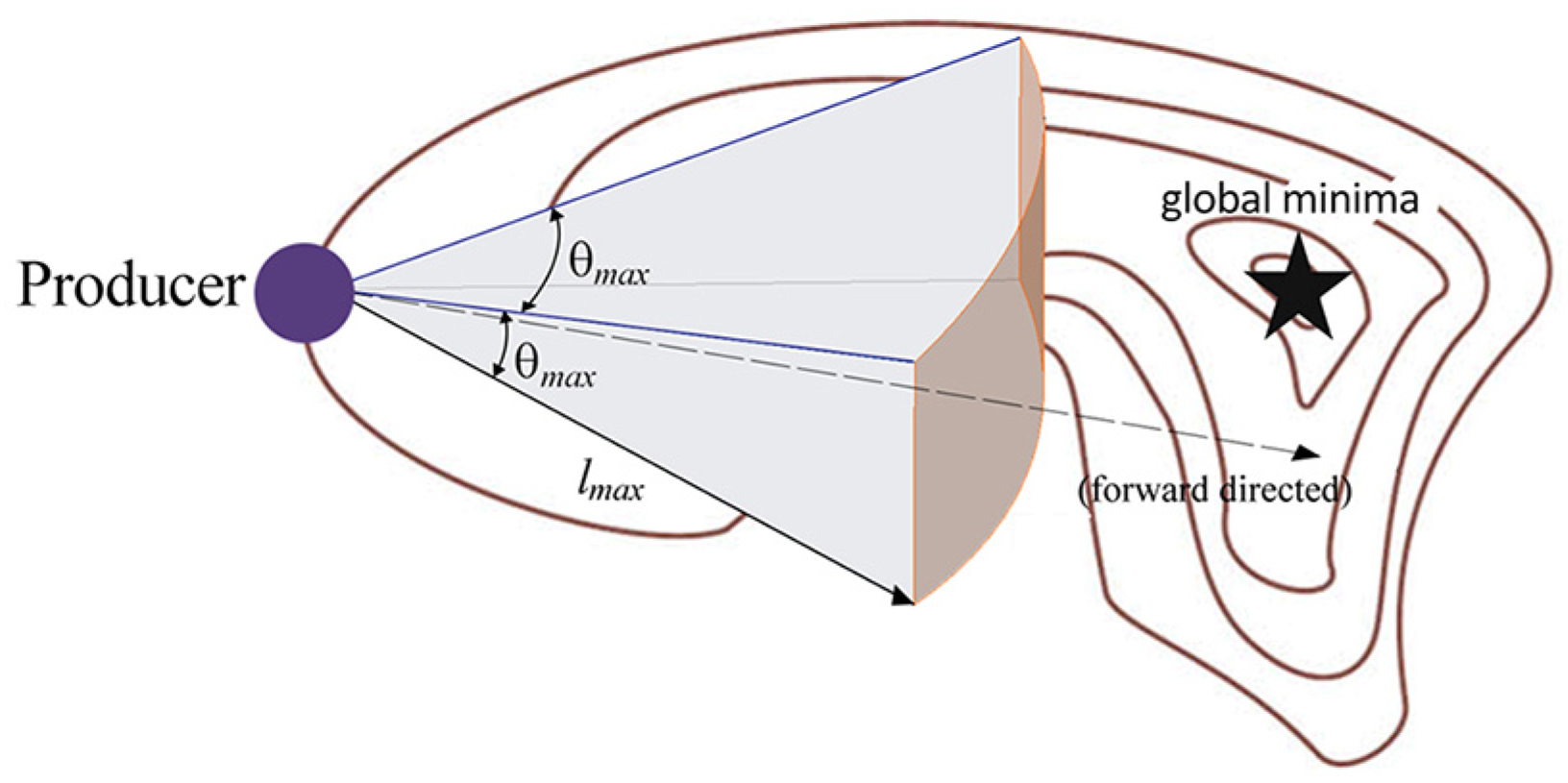
Producers explore the design space by sampling trial solutions along adaptively updated directions (e.g., via variable angles or step lengths), retaining any improvements. In detail, for a generic producer, the scanning field in 3D space can be considered a wedge or a cone (see Figure 10) characterized by the maximum pursuit angle θ_max and the maximum pursuit distance l_max [15,18].

The scanning mechanism of the producer consists of the search at zero degrees (forward direction or z direction), one point on the left side (l direction) and one point on the right side (r direction) of the scanning field. The equations that characterize the scanning mechanism of the producer are shown in [16,17,18,19].

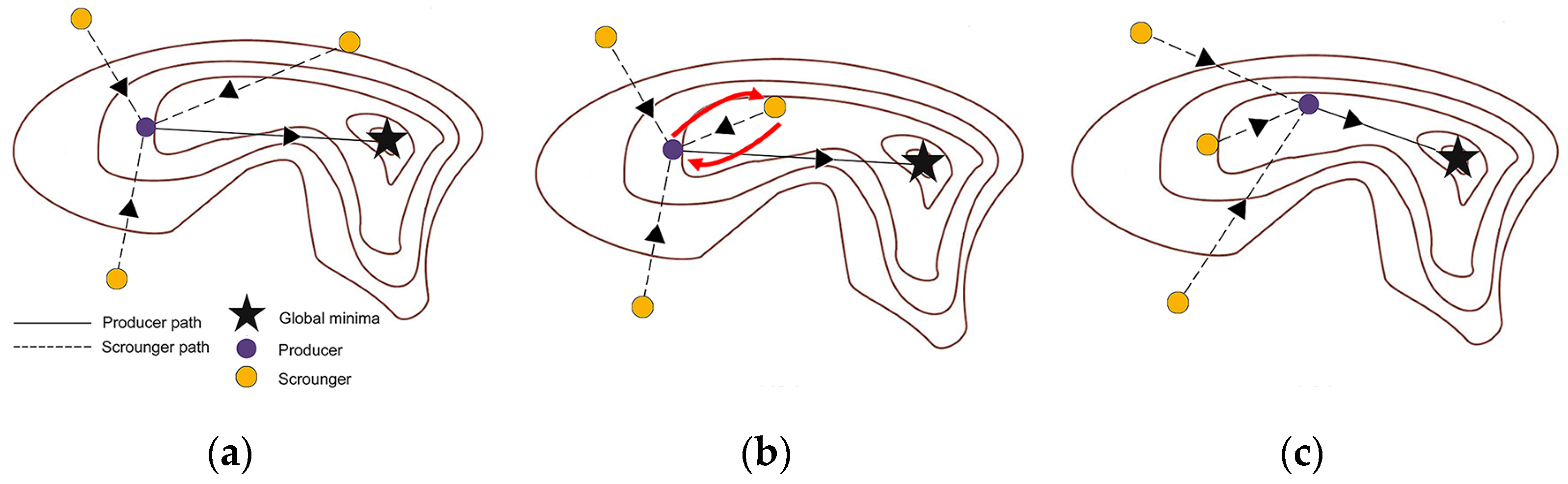
Scroungers exploit these discoveries by generating new candidates through combinations of their current positions with the best Producer positions, thus intensifying the search around high-quality regions. For the scrounging mechanism, in each iteration, all the selected scroungers perform a movement toward the producer. In the generic t-th iteration (Figure 11a), if the algorithm finds a better solution for the scrounger, the software automatically updates the positions of both the producer and the scrounger (Figure 11b). Consequently, in the next iteration, the new producer will be in a better position to reach the objective value (Figure 11c).

Rangers maintain population diversity by performing broader searches. Unlike existing approaches in the literature and in the same way shown for the Firefly Algorithm, in this study, we introduce a novel ranger-selection mechanism with four distinct random-motion modes:

• Global random selection: rangers are chosen at random from the entire search space.
• Producer-centric random selection: rangers are chosen at random from a localized region around the current producer.
• Cycle-by-cycle hybrid selection: in each cycle, a binary flag (0 or 1) is used to decide between the global or the producer-centric modes.
• Periodic hybrid selection: the algorithm alternates between global and producer-centric selection every k cycles, where k is a user-defined interval.

Each mode can be activated automatically, allowing flexible exploration of the search space. At each iteration, candidate designs are checked by the software for feasibility against all constraints, and the objective function is evaluated. The best solution to date, along with the type of member who determined the best solution, iteration number, and cumulative CPU time, is recorded in the optimal solution array. The algorithm terminates under the same criteria used for the GA and the FA.

5. Numerical Analyses

Numerical simulations were carried out in the ANSYS environment through fully parametric scripts that automate the implementation of the three algorithms (GA, FA, and GSO). Each model was discretized using PIPE181 elements, and a preliminary mesh-convergence study was performed by successively refining element sizes. This procedure ensured that the subsequent optimization results reflect true algorithmic performance rather than discretization error. In all analyses conducted, a maximum number of iterations, N_lim = 200, was imposed. All analyses were performed on a PC equipped with a 12th Gen Intel^® Core™ i9-12900H 2.50 GHz processor and 64 GB of RAM.

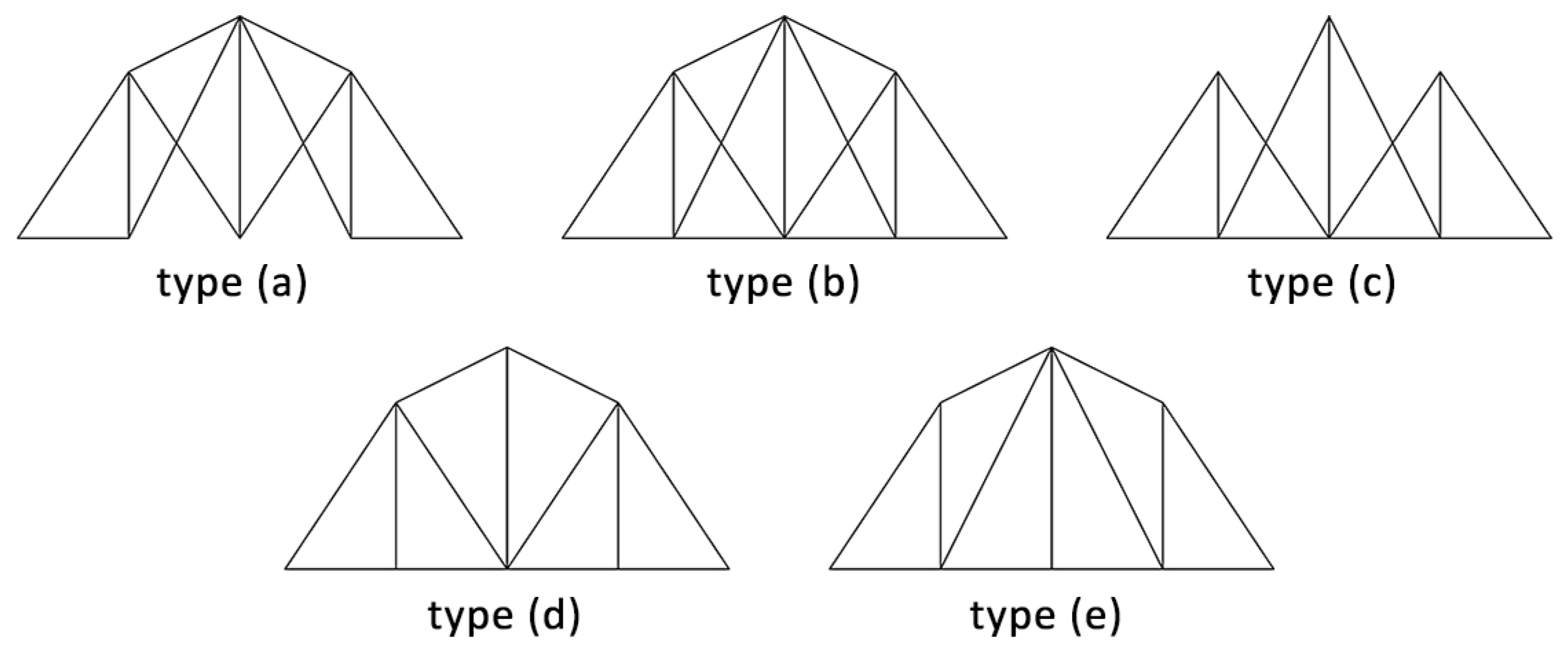
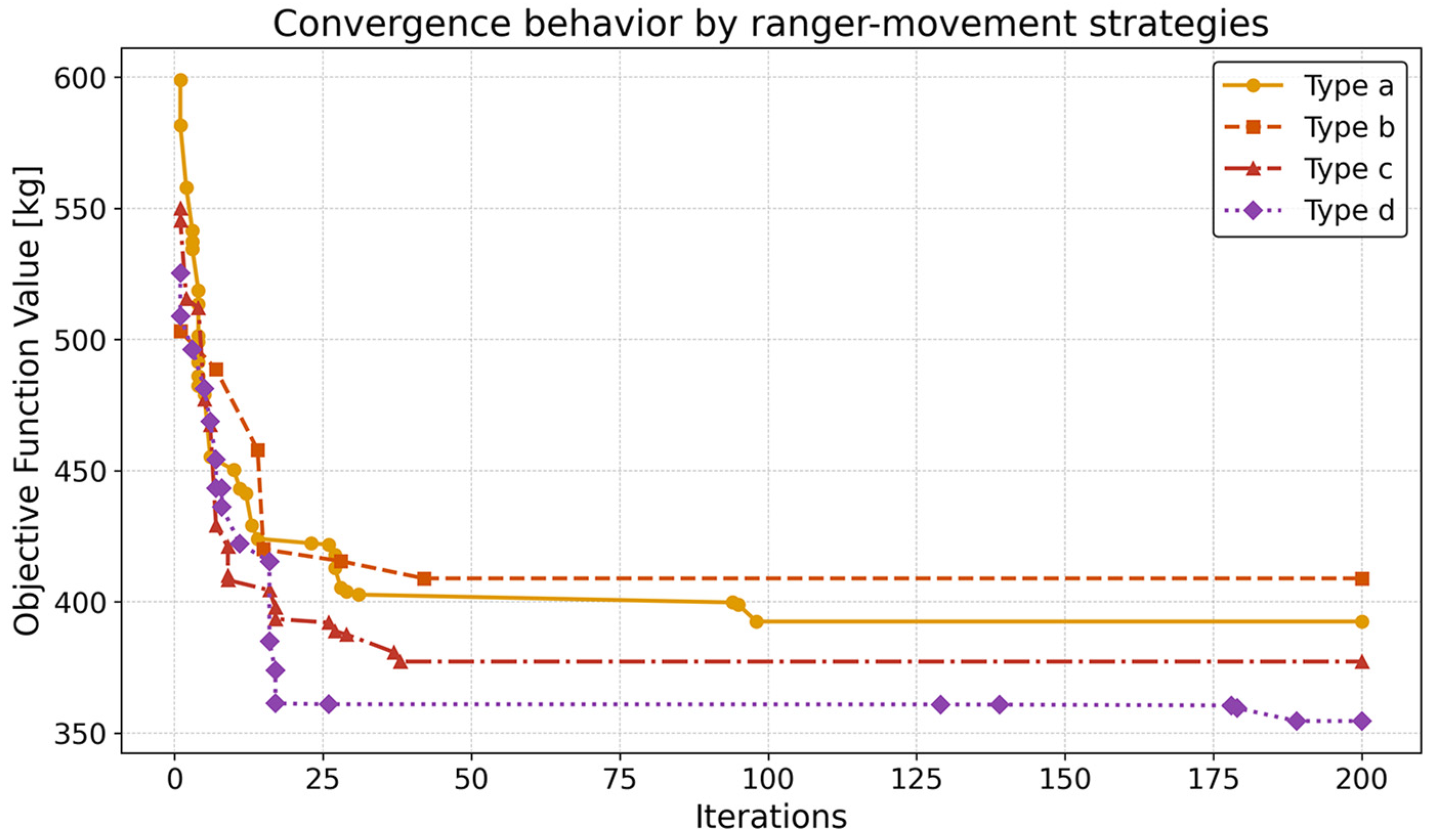
The first analyses concerned a series of preliminary tests designed to identify which of the four ranger-movement strategies (type a, b, c, or d) delivers the most effective solutions. Using the GSO algorithm in the case A study, Figure 12 plots the objective function value versus the number of iterations for each ranger movement type. Among the four approaches, the periodic hybrid strategy (type d) consistently produced the lowest objective function values.

As shown in Figure 12, the periodic hybrid scheme (type d) not only converges rapidly but also produces the lightest design. By iteration number 20, it has already reached a weight just 2% above the overall minimum achieved in the simulation. Moreover, the final weight is 14% lower than that achieved with the producer-centric strategy (type b), 10% lower than with pure global random moves (type a), and 6.4% lower than with the cycle-by-cycle hybrid (type c). Accordingly, this configuration was adopted for all subsequent analyses.

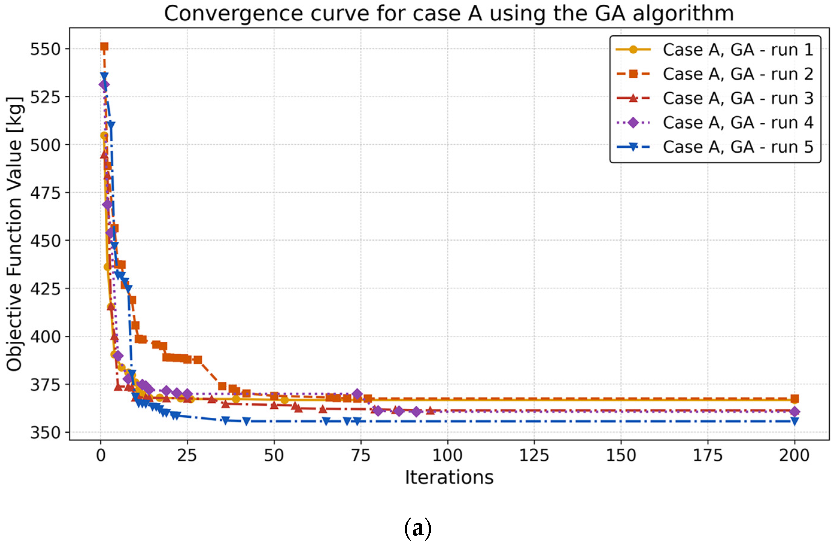
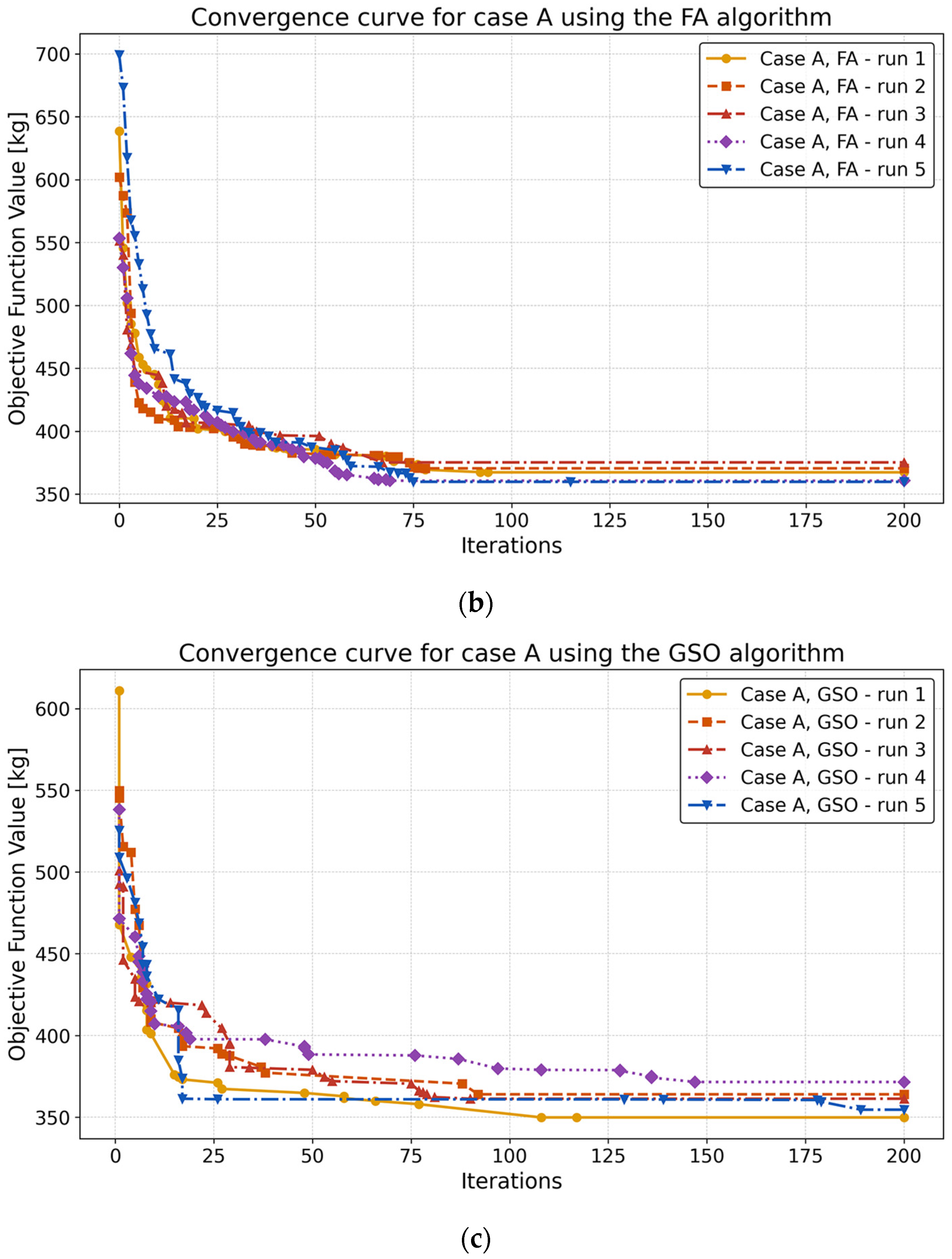
Figure 13 shows the convergence curves for case A obtained, respectively, with the GA, FA, and GSO algorithm. Each optimization was repeated five times. The plots show that all three methods reach their respective optima within 200 iterations. The lowest weight W_min = 349.9 kg is achieved by GSO.

The following figure, Figure 14a, compares the mean final weights of the optimized structures obtained from five independent runs of each optimizer. The figure also shows the standard deviation error bars. In relative terms, the mean weight obtained with GSO is about 0.6% lighter than GA and about 1.5% lighter than FA. In terms of dispersion, FA exhibits the greatest variability, whereas GA yields the narrowest spread of the mean final weights. Although the three algorithms differ in mean weight by less than 1.5%, GSO combines the lowest mean weight with an intermediate standard deviation, underscoring its suitability for this structural optimization task.

This result is corroborated by the time-based trends shown in Figure 14b. For clarity, the graph shows only the best-performing run of each optimizer (GA, FA, and GSO). While all three methods converge to nearly the same optimal weight, their computational costs vary significantly. GSO completes the analysis in just over 24 min, the FA in approximately 36 min, and the GA in about 44 min. The GA is the slowest, requiring 22% more time than the FA and 83% more time than GSO to execute 200 iterations.

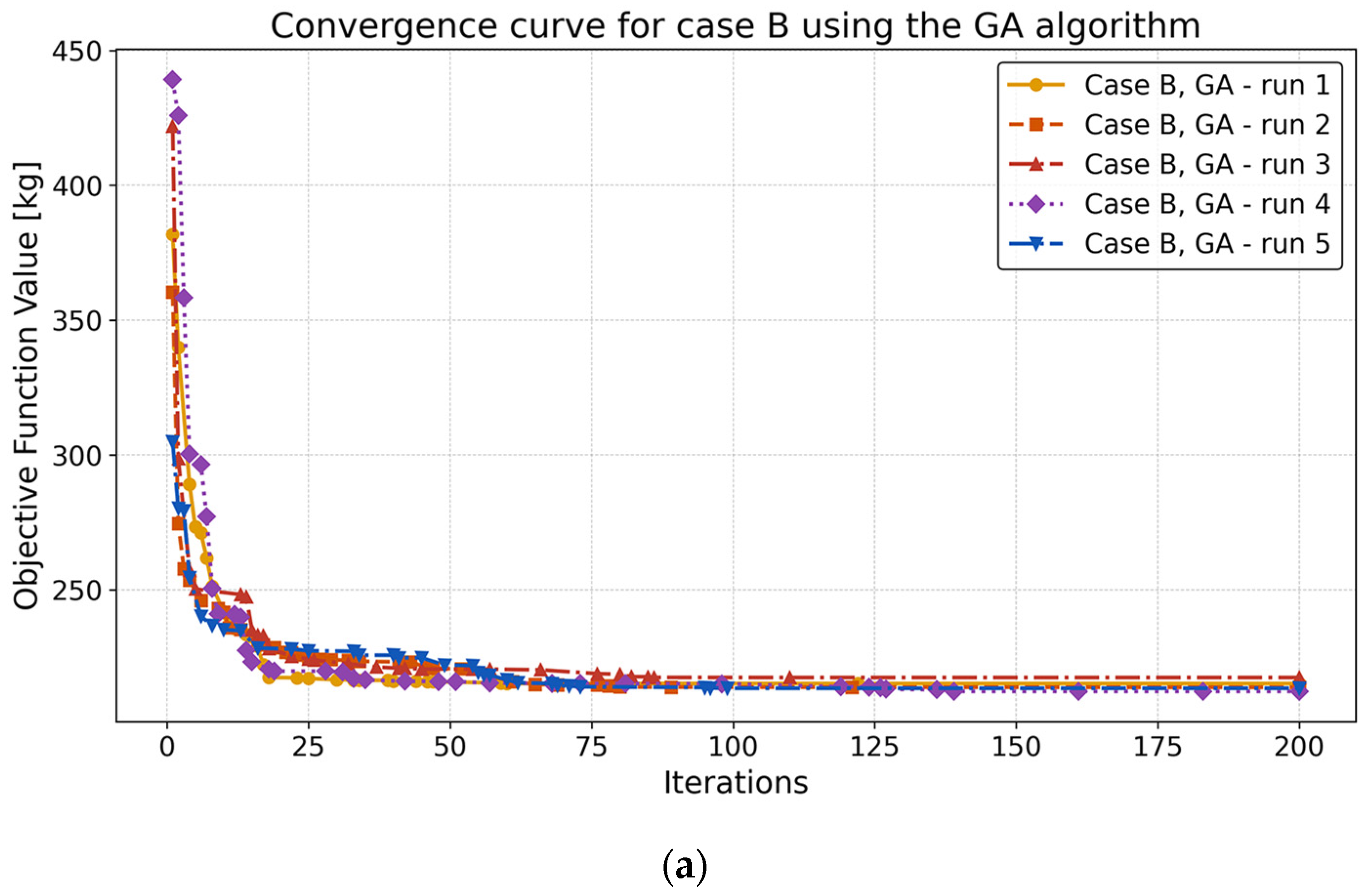
Figure 15 shows the convergence curves from five independent runs for the case B study. The trends show that both GA and GSO achieve the best final value (W_min = 212.35 kg), outperforming FA in terms of solution quality.

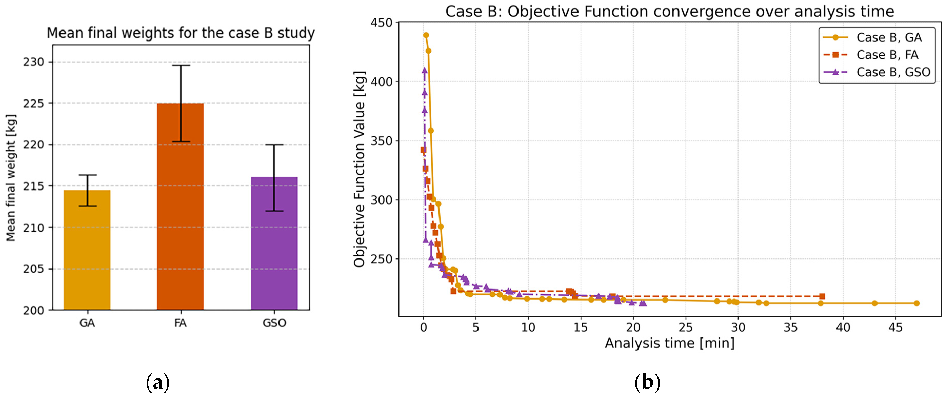
Figure 16 summarizes the obtained results for the case B study. In particular, Figure 16a compares the mean final weights from five independent runs of each optimizer, while Figure 16b plots the objective function value over the analysis time.

Comparing the two graphs in Figure 16, the Genetic Algorithm yields the lightest structures on average but at a substantially higher computational cost. Specifically, GA requires approximately 81% more time than GSO and 24% more time than FA to reach its optimum. FA, in turn, takes about twice as long as GSO to converge. Definitively, GSO achieves a nearly equivalent final weight (within 1%) yet converges in less than half the time of GA and just over half the time of FA. Thus, in this case study as well, GSO proves the most efficient choice when both weight minimization and run time are critical.

Figure 17a,b show the optimized structures obtained in ANSYS, respectively, for case study A and case study B.

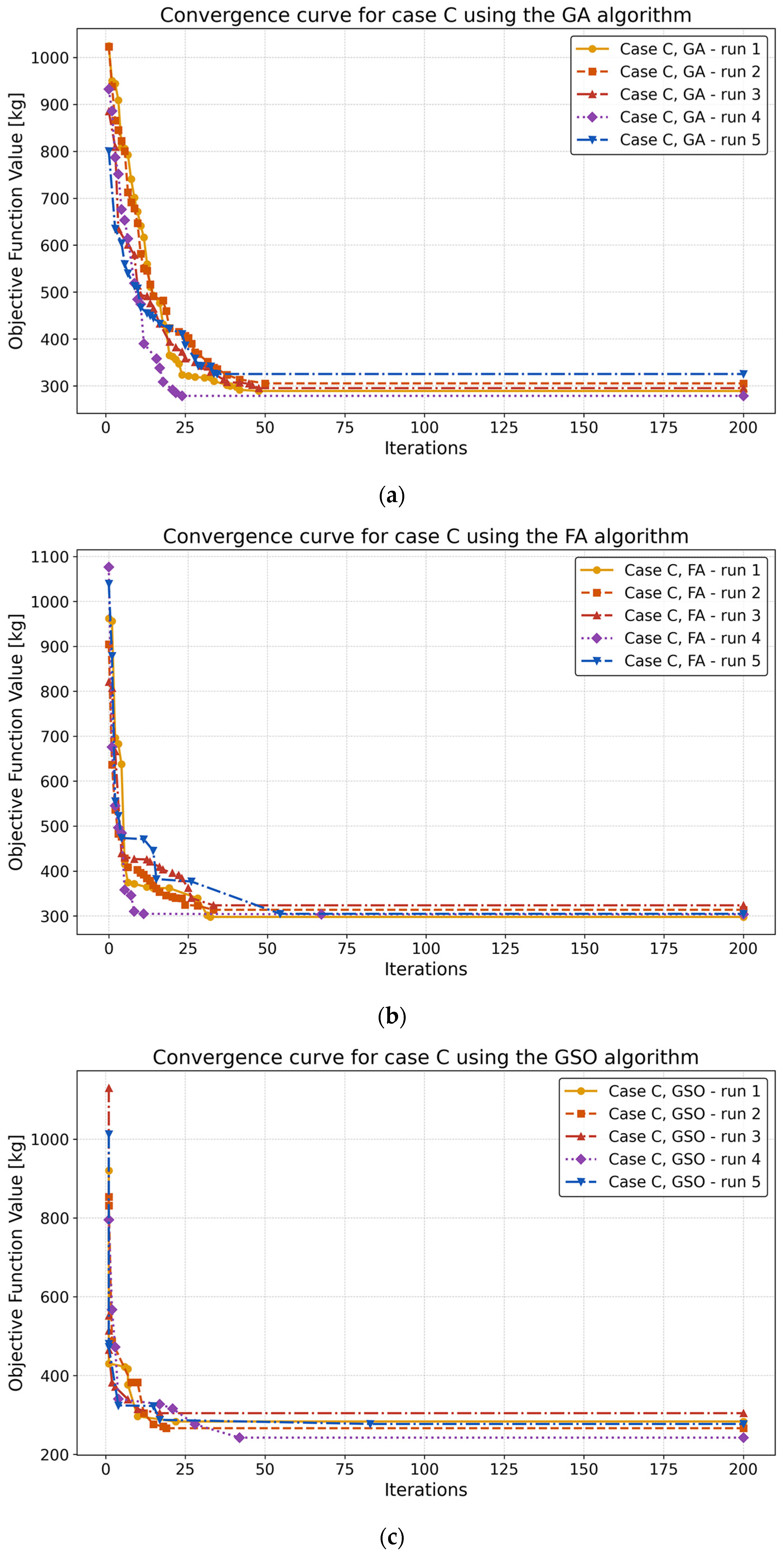
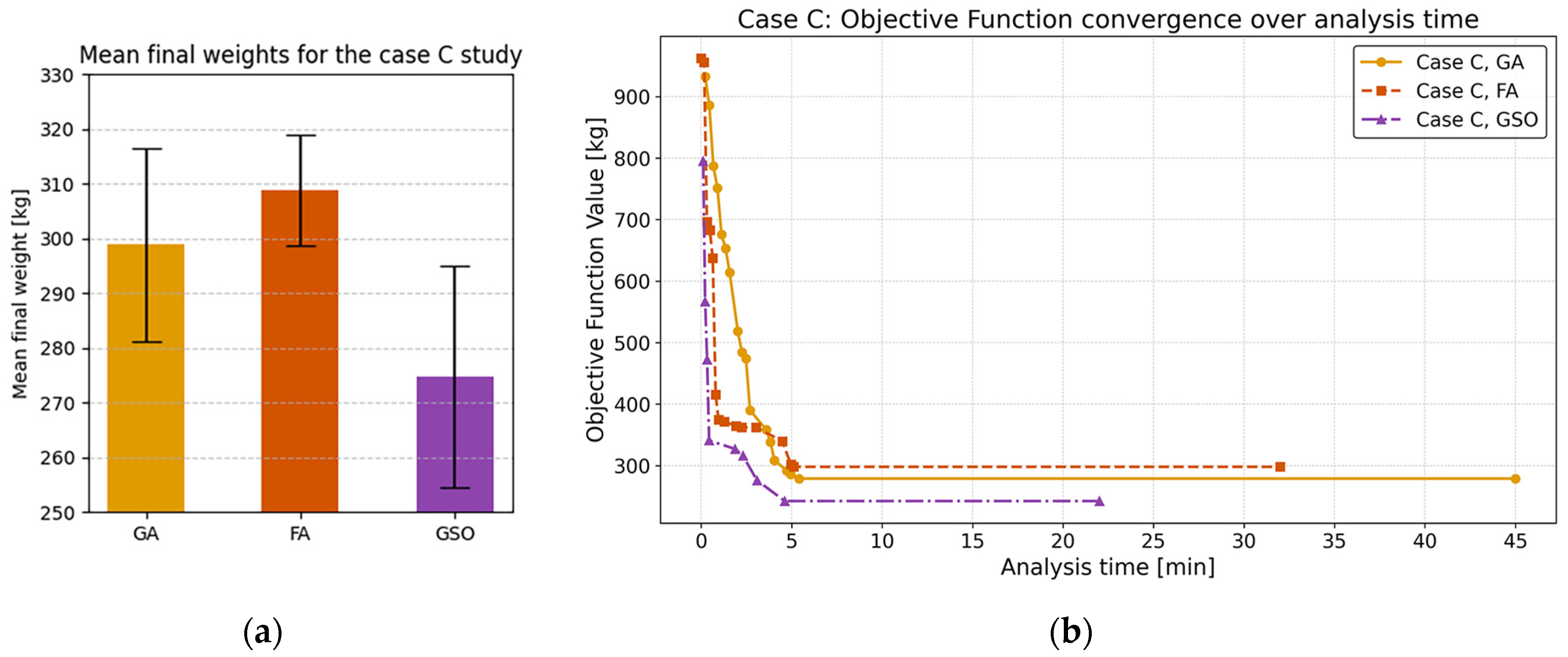
The third case study (case C) presented the greatest challenge, as it involved simultaneous optimization of both member dimensions and internal topology. Figure 18 shows the convergence curves for all three algorithms.

The lightest configuration, with a minimum weight of W_min = 242.41 kg, was obtained by the GSO algorithm. Averaged over five independent runs, the GSO result is approximately 12% lighter than that of FA and 8% lighter than that of GA (Figure 19a). As before, the GA remains the slowest to converge (Figure 19b), requiring up to 104% more computational time than GSO and up to 40% more time than FA to reach its optimum.

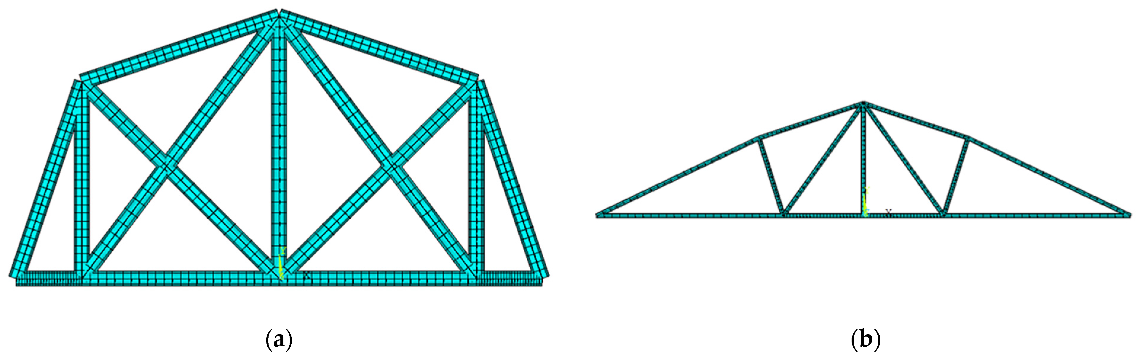
The initial configuration used for comparison in Case C was deliberately set to represent the heaviest feasible structure: all bars were active, and the cross-sectional dimensions were at their maximum values (see Figure 20a). This setup aims to clearly highlight the potential of the optimization process. The final optimized configuration is shown in Figure 20b. In detail, the redesigned structure weighs 95% less than the initial model and exhibits a markedly reconfigured internal topology.

6. Discussion and Conclusions

In this work, a comparative investigation of three nature-inspired metaheuristic optimizers, implemented entirely within the native APDL environment of ANSYS, is presented. While literature studies have demonstrated the effectiveness of these algorithms when coupled to ANSYS via external tools (Python, MATLAB, C++ scripts, etc.), no widely documented study exists on implementing these algorithms exclusively within ANSYS APDL. By integrating each metaheuristic directly into APDL routines, seamless interaction with the ANSYS solver was ensured, interprocess communication overhead was eliminated, and full control over the simulation workflow was maintained. These advantages translate into substantial savings in computational effort without compromising solution quality.

To validate the proposed approach, three benchmark truss structures under prescribed loading conditions were selected: a 22-bar spatial truss (Case A), a 25-bar spatial truss (Case B), and a two-dimensional, 15-rod truss in which topology variables are handled via a Discrete Topology (DT) method (Case C). The DT formulation, in particular, reduces the number of allowable topologies to a finite set of mechanically feasible configurations, thereby narrowing the search space and accelerating convergence. Before addressing these case studies, a preliminary calibration of the GSO algorithm was conducted, testing four alternative ranger-movement strategies. It was found that the so-called “periodic hybrid” scheme (whereby rangers alternate between directed, distance-based steps and randomized exploratory jumps) yields the fastest convergence and the highest-quality objective function values across multiple simulation runs.

Regarding the Firefly Algorithm (FA), the original formulation does not incorporate randomly moving fireflies explicitly. However, in this study, an analogous, adaptive random movement strategy was adopted for FA to enhance the exploration capabilities and consequently improve the likelihood of discovering better solutions.

When applied to cases A, B, and C, all three metaheuristics successfully located structurally sound, lightweight configurations. However, their computational profiles and final weights diverged in meaningful ways. In every instance, GSO reached its optimal or near-optimal solution in a fraction of the CPU time required by GA. Although GA occasionally achieved a marginally lower mean final weight, this tiny improvement came at a run-time penalty ranging from 80% to 100% compared to GSO. FA occupied an intermediate position: its final configurations were typically 1–4% heavier than GSO’s, and its CPU time was roughly double that of GSO in most runs. In other words, FA succeeded in balancing solution quality and computational cost, but GSO’s adaptive ranger movements provided a decisive advantage, rapidly guiding search members toward promising regions of the design space without excessive exploration overhead.

A closer examination of the convergence trajectories reveals why GSO excels. The hybridized ranger movement alternates between a directed step (which exploits known promising areas) and a random jump (which preserves global diversity). This dynamic modulation of “exploration versus exploitation” avoids the common pitfalls of stagnation in local minima. By contrast, GA’s reliance on fixed-probability crossover and mutation can lead to a slower spread of favorable genetic material, especially as the search nears convergence. FA’s stochastic attraction mechanism, while effective for escaping shallow traps, still requires more iterations (and thus more finite element analyses) to home in on the global optimum. In summary, the enhanced convergence speed of GSO (validated by both objective–value curves and CPU–time comparisons) supports its recommendation as the first choice for structural-weight minimization when both accuracy and run-time efficiency are critical. Beyond raw performance, the native APDL integration itself proved to be a key contribution. By embedding the optimization logic within APDL, file-based data exchange was eliminated, Python-to-ANSYS calling overhead was avoided, and the ANSYS solver state was preserved between iterations.

In conclusion, this comparative study highlights two main takeaways. First, among the three metaheuristics, GSO with adaptive ranger movements offers the best trade-off between convergence speed and final weight, followed by FA and then GA. Second, implementing these algorithms directly in APDL not only simplifies workflow integration but also yields measurable gains in computational efficiency—benefits that are especially evident in large-scale, high-fidelity structural models. Future work will explore extending the APDL-based framework to multi-objective formulations (e.g., incorporating both weight and stiffness) and to other structural domains, such as shell or solid-element topologies.