Abstract
A full-cycle, multiscale analysis technique was developed for periodic lattice structures with geometric repetition, aiming for more efficient modeling to predict their failure loads. The full-cycle analysis includes both upscaling and downscaling procedures. The objective of the upscaling procedure is to obtain the effective material properties of the lattice structures such that the lattice structures can be analyzed as continuum models. The continuum models are analyzed to determine the structures’ displacements or buckling failure loads. Then, the downscaling process is applied to the continuum models to determine the stresses in actual lattice members, which were applied to the stress and stress gradient based failure criterion to predict failure. Example problems were presented to demonstrate the accuracy and reliability of the proposed multiscale analysis technique. The results from the multiscale analysis were compared to those of the discrete finite element analysis without any homogenization. Furthermore, physical experiments were also conducted to determine the failure loads. Then, multiscale analysis was undertaken in conjunction with the failure criterion, based on both stress and stress gradient conditions, to compare the predicted failure loads to the experimental data.
1. Introduction
Many engineering materials and structures have repetitions in their geometries or constituent materials. Fibrous or particulate composite materials are examples of repetitive constituent materials, while truss and frame structures are examples of repetitive lattice geometries. Mechanical metamaterials also have forms of lattice structures of repetitive geometries. One example is the auxetic structure with a negative Poisson’s ratio [1,2,3,4,5,6,7,8].
When materials and structures contain many repetitions, the homogenization process is applied to them to simplify their analyses. The repeated constituent materials and geometries are smeared and replaced by a homogeneous continuum with effective material properties, which may be isotropic or anisotropic. For instance, macroscopic composite material properties are determined by homogenizing the reinforcing and binding materials. Generally, fibrous composites result in anisotropic effective material properties while particulate composites yield isotropic effective material properties. Extensive research has been conducted on the homogenization of composite materials [9,10,11,12,13].
Lattice structures have many repetitive arrangements of lattice members. For example, the truss structure has repetitive triangular shapes in the arrangement of lattice members. The lattice structures can be analyzed analytically if simple enough or numerically using the finite element method otherwise. However, if the lattice structures have so many lattice members, it is time-consuming to analyze them with the discrete modeling of every lattice member because the computational time is nonlinearly proportional to the number of degrees of freedom in the model. This statement is even more true if the analysis needs to be repeated so many times to optimize the structures. Thus, homogenization techniques have been developed to determine the effective material properties of the lattice structures with many repetitive forms of lattice members [14,15,16,17]. Then, the lattice structures can be modeled as continuous media with much smaller degrees of freedom to save computational time. Excellent surveys were undertaken for homogenization research on lattice structures [18,19].
The homogenization techniques were classified into several categories based on the models used for homogenization [19]. For example, there were the beam model [14,15,16,20,21], equivalent strain energy model [22,23], asymptotic homogenization technique [24], and multiscale approach [25]. Analytical, numerical, and/or machine learning techniques can be utilized for the homogenization process. In addition, the current multiscale technique [26] uses different length scale models in the same analysis without explicit upscaling and downscaling processes.
All the previous homogenization techniques determined the effective stiffness of the lattice structures to compute their displacements or buckling failure. However, there were few attempts to calculate the actual stresses in the lattice members to predict excessive stress failure, to our best knowledge. Thus, this study proposes a full-cycle multiscale analysis technique for lattice structures made of beams, which can compute not only the displacements but also the strain, stress, and predict potential failure of actual lattice members due to excessive stresses.
The full cycle of the multiscale analysis is sketched in Figure 1. It consists of the upscaling and downscaling processes [27]. The upscaling process is the homogenization process, which was studied extensively as discussed above. In other words, the discrete lattice structures are smeared into homogenized continuum models. Then, the latter is analyzed using the finite element method to determine the deformations and displacements of the homogenized models. After that, the downscaling process is applied to the solutions of the homogenized models to extract stresses and strains in actual lattice beam members. Such a downscaling process has been investigated very rarely in the past. Finally, failure criteria based on both stress and stress gradient conditions are applied to those stresses or strains to predict potential failure. If the load is applied incrementally, the multiscale procedures repeat for every incremental loading with progressive failure in the lattice structure.
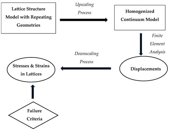
Figure 1.
Full-cycle multiscale analysis scheme.
The following sections describe in detail the upscaling and downscaling techniques. A recently proposed failure criterion is followed. Then, numerical examples of lattice structures are presented. The solutions of the multiscale technique are compared to those of the discrete lattice structure models that include explicitly every lattice member. The comparison includes both displacements and stresses, which were obtained from the upscaling and downscaling processes, respectively. Furthermore, the failure criterion is applied to the computed stresses at the lattice members to predict the failure loads of lattice structures. To validate the predicted failure loads, experiments were conducted for the lattice structures that were prepared using a 3-D printer with a polymer material. Finally, a summary and conclusions are provided at the end.
In the following derivation, the material is assumed linear elastic and isotropic. Furthermore, a small deformation is assumed for simplicity. However, the generality of the analysis framework is not necessarily confined to the assumptions.
2. Upscaling Technique
Figure 2 shows a lattice structure made of periodic rectangular cells. The unit cell of the lattice structure is also shown in the same figure, and Figure 3 shows the enlarged unit cell with the length l and the width w. The unit cell lattice is taken from the center of one lattice to the center of the next lattice. Thus, the thickness of the unit cell lattice in Figure 3 is t/2 because it is half of the thickness of the lattice structure in Figure 2, which is equal to t.
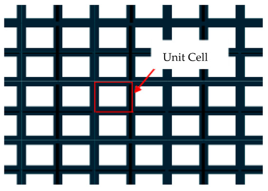
Figure 2.
Lattice structure consisting of rectangular open cells.
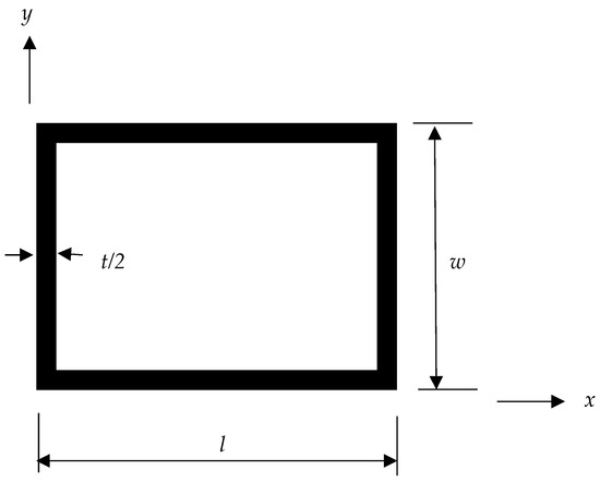
Figure 3.
Unit cell of a rectangular lattice. All the members have the same thickness.
To determine the effective elastic modulus along the x-axis of the unit cell in Figure 3, let us apply a uniform displacement d along the x-axis of the rectangular unit cell to its right side lattice while the left side lattice is constrained from any movement. In that case, the two horizontal lattices at the top and bottom sides provide the major stiffness, while the two vertical lattices on the left and right sides provide negligible stiffness as compared to the horizontal lattices. Thus, the stiffness in the x-axis is
where is the stiffness of the unit-cell lattice in the x-axis, and is the elastic modulus of the lattice material. The homogenized material has the stiffness expressed as below:
where is the effective elastic modulus along the x-axis. The stiffness of the homogenized material should be equal to that of the unit cell lattice, which leads to the following equation:
Equation (3) states that the ratio of the effective modulus along the x-axis to the elastic modulus of the lattice material is equal to the ratio of the total lattice thickness of the horizontal lattices and the vertical dimension of the unit cell. The vertical lattices in the unit cell only act to separate the horizontal lattices by a specific distance. Thus, a change in the length L does not affect the effective modulus along the x-axis. Likewise, the effective modulus along the y-axis is expressed as
If diagonal members are added to the rectangular lattice structure, the corresponding unit cell is shown in Figure 4. Let us first assume that the two diagonal members are independent of each other and do not have a direct connection. Then, as before, a uniform displacement is applied to the right side of the unit cell in Figure 4 while the left side is constrained from any movement. Figure 5 shows the displacement of one of the diagonal members with the applied horizontal displacement. The diagonal member has the original location at OA whose initial length is in which l is the horizontal length of the unit cell, and is the angle between the horizontal and diagonal directions, as shown in Figure 5.
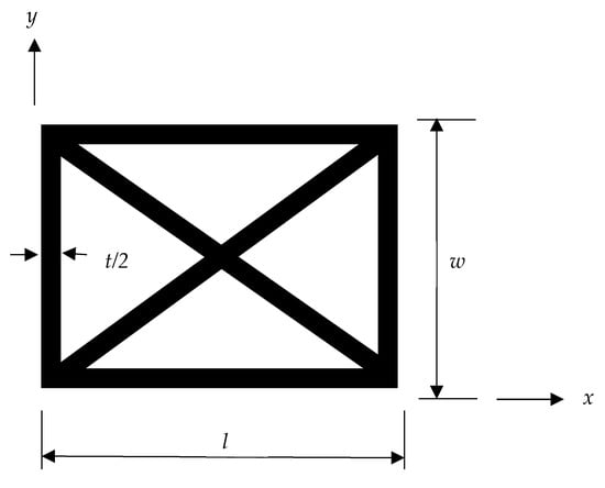
Figure 4.
Unit cell of a rectangular lattice with diagonal members.
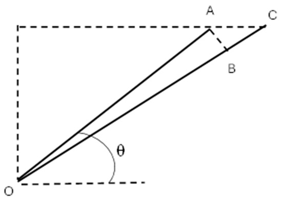
Figure 5.
Displacement of a diagonal member by horizontal elongation of the unit cell in Figure 3.
If AC in Figure 5 is the horizontal displacement , and . Among the two components of the displacement of the diagonal bar from OA to OC, AB is caused by bending loading, while AC results from the axial force. Because the diagonal member has a dimension like a beam with a large slenderness ratio, the bending load for AB is much smaller than the axial force for AC. If the slenderness ratio is close to one, the bending should be considered. As a result, the bending load is neglected. The axial force on the diagonal member to induce the deformation AC is expressed as
where is the thickness of the diagonal member and is the elastic modulus of the diagonal member. If the diagonal member has the same elastic modulus and thickness as those of the horizontal and vertical members of the lattice structures, the horizontal component of the axial force, , is expressed as
Then, the effective modulus of the unit cell with diagonal members becomes
3. Downscaling Technique
The solution of the homogenized structure does not provide stresses in the actual lattice members. The stresses in the homogenized body are mathematically smeared stresses, but not the actual stresses experienced by lattice members. Thus, the downscaling process is conducted to compute the actual stresses in the lattice members because failure would occur in the overstressed lattice members. The lattice members may fail by tensile failure or buckling under compression. The downscaling analysis is conducted using the same unit cell used for the upscaling process.
The lattice members are modeled using beam elements, while the homogenized body is modeled using a continuum element, like plane stress or 3-D solid elements. Therefore, there is a mismatch in the degrees of freedom between the beam elements and continuum elements. The continuum elements do not have rotational degrees of freedom. The downscaling process is to resolve this issue and to compute the stresses in the lattice beam members.
Let us use the rectangular unit cell in Figure 3 and Figure 4 to explain the downscale process. The finite element matrix equation is developed using beam elements for the unit cell. The unit cell may or may not have internal members like the diagonal members, as shown in Figure 3 and Figure 4, respectively. The unit-cell model has four nodes at the corners for Figure 3 and one additional center node for Figure 4. Every node has three degrees of freedom. All the degrees of freedom in the unit cell are classified into two groups. The first group contains the displacement degrees of the corner nodes, which are compatible with the continuum elements. The second group contains all the rotational degrees of freedom and the degrees of freedom other than at the corner nodes. This group is condensed out in the matrix equation as described below.
The stiffness matrix equation of the unit cell is broken down into the following submatrices:
where contains the degrees of freedom of the first group, while Includes the degrees of freedom of the second group. The second row of Equation (8) is written as
Solving Equation (9) for results in the following relationship with the first group :
We compute the displacements at the four corners of the unit cell from the solution of the homogenized model, where we want to calculate the stresses in the lattice members. Next, we compute the values of the condensed degrees of freedom using Equation (10). Finally, both and are substituted into Equation (8) to compute the forces and moments at nodal locations. Lattice stresses are determined by the forces and moments using
Equation (11) gives normal stress to the lattice member. Likewise, shear stress can be computed from the shear load on the lattice member. Equation (11) is for a 2-D lattice element. A similar equation is used for a 3-D lattice element.
4. Failure Criteria
A new failure criterion was proposed recently to predict the failure of different cases, which used to require different failure theories for each case when using the traditional failure criteria. Thus, it was called a unified failure criterion. The new failure criterion is based on two parameters: effective stress and the stress gradient [28,29]. For failure to occur, both stress and stress gradient conditions must be satisfied simultaneously. The two conditions are expressed as
and
where denotes the effective stress, which is different depending on the material characteristics. For instance, the maximum normal stress is used for brittle isotropic materials. For composite materials, multiple effective stresses can be used depending on the composition of the constituent materials, like fiber and matrix materials. is the strength of the material, which is obtained from the uniaxial loading tests. E is the elastic modulus, and is another material property related to the failure of the material. That is equivalent to the critical energy release rate in fracture mechanics [28]. Finally, s is the direction of the failure path. Thus, the failure criterion requires information about not only the failure location but also the failure direction. This failure criterion has been validated extensively for brittle materials under both static and cyclic fatigue loading, and is currently under investigation for its applicability to ductile materials. An initial study showed a very positive result.
If the effective stress has a negligible stress gradient at the failure location, the stress condition of Equation (12) determines the failure load. This is because the effective stress to satisfy the stress gradient condition is smaller than the effective stress to meet the stress condition. For example, this is the case with the uniaxial loading of the standard dog-bone shape specimens, which have zero stress gradient with uniform stress across their width.
On the other hand, if the failure location has a significant stress gradient, like at the edge of a crack or a hole, the stress gradient condition in Equation (13) determines the failure load. In this case, the effective stress from Equation (13) is greater than that from Equation (12). Because both conditions must be satisfied simultaneously for failure to occur, the effective stress from Equation (13) determines the failure load.
The set of failure criteria is applied to the lattice members that would fail. The maximum longitudinal stress is determined from Equation (11) for the lattice member that carries the maximum internal load. That stress in Equation (11) is used for potential failure with the stress condition of Equation (12). The stress gradient is also computed from Equation (11), and it is . This stress gradient varies along with the internal moment M. To make the stress gradient independent of the magnitude of the applied loading, the gradient value is normalized in terms of the unit stress at the location of potential failure. Then, the normalized stress gradient is expressed as
where F and M are the internal force and moment applied to the lattice member under consideration for failure, t is the thickness of the lattice member, and denotes the normalized stress with a unit value like 1 Pa. Equation (14) is used for the stress gradient failure condition of Equation (13). Structural members subjected to both axial and bending loads fail due to the stress gradient condition. That is, the failure stress from the stress gradient condition is greater than that from the stress condition. To satisfy both conditions simultaneously for failure, the induced stress must exceed or be equal to the failure stress from the stress gradient condition.
5. Examples and Discussion
Two-dimensional lattice structures were studied for both their displacements and induced stresses. The first structure is a cantilever beam with a transverse force at its end, as shown in Figure 6. The ratio of the beam length to thickness, L/H, varied from 20 to 80. The cantilever beam was made of a lattice structure with the unit cell as shown in Figure 3 or Figure 4. That is, the first structure had a rectangular shape of lattices, and the second structure had both rectangular shapes of lattices along with two diagonal internal members.
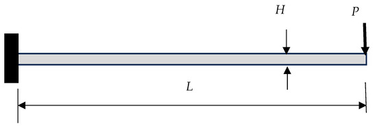
Figure 6.
Cantilever beam with a force at the tip.
The homogenization technique was used to determine the effective material properties of the lattice structures. Then, the effective material properties were used to determine the tip deflection of the cantilever beam using the analytical solution, which is
where is the tip deflection of the cantilever beam, P is the applied force at the tip, L is the length of the beam, is the homogenized elastic modulus, and is the second moment of inertia of the cross-section of the homogenized beam. The tip deflection of the homogenized beam was compared to the tip deflection of the original lattice structure, which was solved using the finite element method with beam elements for every lattice member.
Table 1 compares the tip deflection between the homogenized model and the discrete lattice structure model for different cantilever lengths and geometric dimensions of lattice members, with the unit cell shown in Figure 3 without diagonal lattice members. The unit cell has a square shape with w/l = 1. Equation (3) was used for the homogenized model’s effective modulus in Equation (15). The discrete model included every lattice member in the analysis. The table shows the ratio of the tip deflection of the homogenized model to that of the discrete lattice structure model. If the upscaling process is reliable, the ratio of the tip deflection must be very close to 1.

The tip deflection of the homogenized model was very close to that of the discrete lattice model, as shown in Table 1. The result also showed that the homogenized model is closer to the discrete model as the former contains more unit cells. In other words, as more lattice members are smeared into the homogenized model, its deflection is closer to that of the discrete model. This was expected because the discrete model becomes homogenized as the number of lattice members approaches infinity. Thus, the results confirm the convergence of the upscaling process, i.e., the homogenization model.
Overall, the difference between the discrete and homogenized models was less than 5%, except for one case with 8%. The latter case had a smaller number of repeated unit cells in the homogenized model with t/l = 0.2. As the ratio t/l becomes larger, the representative beam length in the unit cell becomes shorter, which results in a larger error. However, such a corrective action was not conducted here to reduce the error because that was not the major objective of the study. As the shape of the unit cell was changed from square to rectangle, the tip deflection of the cantilever beam was compared in Table 2 between the homogenized and discrete models. Both deflections agreed well, too.
Table 2.
Results of the cantilever made of the rectangular unit cell of Figure 3.
The next example was the unit cell shown in Figure 4, which had two diagonal lattice members. The comparison of the tip deflection between the homogenized and discrete models is provided in Table 3. Equation (7) was used for the homogenized model. The deflection of the homogenized model was close to that of the discrete model for both square and rectangular shapes of unit cells.
Table 3.
Results of the cantilever made of the unit cell of Figure 4.
For the downscaling process to determine the maximum stresses at the actual lattice member, the displacements were obtained from the homogenized model at the top, left corner of the cantilever, as shown in Figure 7. The displacements at the four corners of the square or rectangular shape with the unit cell size were determined from the homogenized model. Those displacements are equivalent to the group in Equation (10), which is used to determine the group in that equation. Once both and are computed, Equations (8) and (11) are used to determine the stresses at the lattice members. The maximum stress occurs at the top lattice member of the unit cell for the cantilever beam with a tip load.
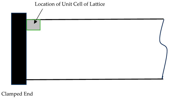
Figure 7.
Selected unit cell location of the cantilever beam for the maximum lattice stresses.
Table 1, Table 2 and Table 3 show the comparison of the maximum stress in the homogenized model to that of the discrete lattice structure model. Overall, the downscaling process yielded lattice stresses very close to those computed directly from the finite element analysis of the discrete lattice structure. The accuracy of the stress from the multiscale analysis was very comparable to that of the displacement. This suggests that both upscaling and downscaling processes are reliable to extract the actual solution of the discrete lattice structure with much less computational time.
The next example was a clamped beam at both ends with a force at the center, as sketched in Figure 8. The lattice structure had the unit cell, as shown in Figure 4. That is, the structure had both diagonal lattice members. Table 4 shows the comparison of the deflection at the center of the homogenized model to that of the discrete model. The homogenized model gave very comparable deflections to the discrete model. However, the accuracy of the homogenized model was better for the cantilever beam than the clamped beam at both ends.
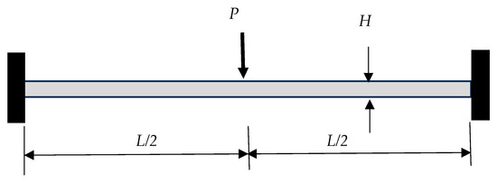
Figure 8.
Clamped beam at both ends with a force at the center.
Table 4.
Results of the clamped beam made of the unit cell shown in Figure 4.
The maximum stress was also compared for the beam clamped at both ends between the multiscale analysis and the discrete finite element analysis of the lattice structure. Table 4 shows the comparison. Both results compare well. The accuracy of the stress prediction depends on the accuracy of the homogenized model because the displacements of the homogenized model are used for the downscaling process to compute the stresses in actual lattice members. Table 4 also suggests that the multiscale analysis resulted in the stresses as accurate as the displacements. This means the downscaling process is very reliable for determining the stresses in the lattice members.
The last set of studies was to predict the failure load of lattice structures using the multiscale technique and the failure criterion as presented in previous sections. The lattice structures were made of unit cells with diagonal members, and they were subjected to three-point bending loads. The length of every lattice structure was 140 mm, and the span length between the two simple supports was 100 mm. Every unit cell had a dimension of 5 mm × 5 mm. The heights of the lattice structures varied from 20 mm to 40 mm with an increment of 10 mm. Thus, the lattice structures had 4, 6, or 8 unit cells across their heights, respectively. The thickness of all the lattice members was 0.7 mm except for the lattice members at the outside boundary of the structures, which were 0.6 mm thick. These lattice structures were fabricated using a fused filament fabrication 3-D printer using the polylactic acid (PLA) material. This material was selected because it is a brittle material with consistent material properties after printing. The printing nozzle and bed temperatures were 200 °C and 60 °C, respectively. The infill density was 100% with a printing speed of 100 mm/s. The line width and layer height were 0.4 mm and 0.15 mm, respectively. The elastic modulus was 2.7 GPa. Figure 9 shows a lattice beam structure with four unit cells along the height after bending failure. As expected, failure occurred at the tensile side of the beam at the center, which has the largest bending stress under three-point bending.
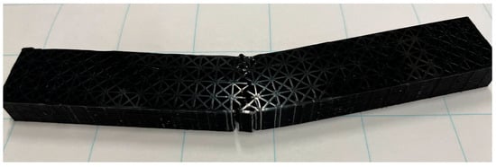
Figure 9.
Bending failure of a lattice structure specimen with four unit cells along the height.
Three or four lattice structures were tested for each different height to determine the average failure loads. All the lattice members were subjected to combined axial and bending loads. Thus, the stress gradient condition determines the failure load. That is, Equation (14) was used to compute the stress gradient, and Equation (13) was used to predict failure stress. Figure 10 compares the predicted failure loads to the experimental results. Because of some unavoidable variation in the thickness of the 3-D printed lattice members, the experimental data showed some scattering. Even though the average thickness of inner members was 0.7 mm, there were some variations from one member to another. The predicted failure loads from the proposed failure theory agreed well with the experimental data. All the predicted failure loads were within the standard deviation of the test data.
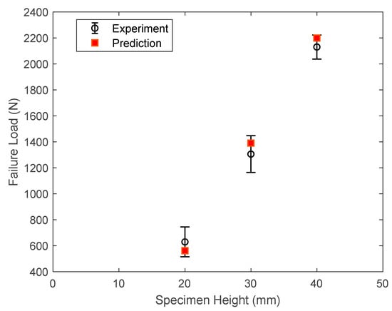
Figure 10.
Comparison of experimental and predicted failure loads.
6. Summary and Conclusions
If a lattice structure consists of many periodic geometries, finite element analysis with modeling every lattice member is very time-consuming. To address this issue, a full-cycle multiscale analysis technique was proposed for lattice structures made of beams. The multiscale technique can determine both stiffness and stress of the lattice structure efficiently and accurately.
To verify the multiscale analysis technique, both displacements and stresses were compared between the results obtained using the multiscale analyses and the detailed finite element analyses for multiple example problems. Those were the cantilever beam and the beam clamped at both ends. Those beams were constructed with square or rectangular shapes of lattice structures with or without diagonal lattice members. The size of those beams and the geometric configuration of internal lattice members were varied. Both upscaling and downscaling processes were assessed individually. The full-cycle multiscale analysis gave very accurate displacements and stresses as compared to those of the detailed finite element analyses.
Furthermore, experiments were conducted on lattice structures to determine their failure loads, which were also predicted using multiscale analysis with the recent failure criterion. It uses both stress and stress gradient conditions to predict failure. Because the lattice members were subjected to both axial and bending loads, the failure was governed by the stress gradient condition. The predicted failure loads agreed well with the experimental values.
Even though this study was focused on 2-D lattice structures, the proposed full-cycle multiscale analysis methodology can be extended to 3-D lattice structures with a 3-D unit cell model. If a lattice structure has a buckling failure mode, that can be predicted from the lattice members under compressive loading. The next study is the application of the current multiscale framework to 3-D auxetic structures to predict their failure loads.
Author Contributions
Conceptualization, Y.K.; analysis and methodology, Y.K.; specimen preparation and testing, M.M.; data validation, Y.K. and M.M.; writing—original draft preparation, Y.K.; writing—review and editing, M.M.; supervision, Y.K.; project administration, Y.K.; funding acquisition, Y.K. All authors have read and agreed to the published version of the manuscript.
Funding
This research was funded by the Office of Naval Research, and the funding document number is N0001424WX02019.
Institutional Review Board Statement
Not applicable.
Informed Consent Statement
Not applicable.
Data Availability Statement
All the data are included in the paper.
Conflicts of Interest
The authors declare no conflicts of interest.
References
- Evans, K.E. Auxetic Polymers: A New Range of Materials. Endeavour 1991, 15, 170–174. [Google Scholar] [CrossRef]
- Evans, K.; Alderson, A. Auxetic materials: Functional Materials and Structures from Lateral Thinking! Adv. Mater. 2000, 12, 617–628. [Google Scholar] [CrossRef]
- Körner, C.; Liebold-Ribeiro, Y. A Systematic Approach to Identify Cellular Auxetic Materials. Smart Mater. Struct. 2014, 24, 025013. [Google Scholar] [CrossRef]
- Lakes, R.S. Foam Structures with a Negative Poisson’s Ratio. Science 1987, 235, 1038–1040. [Google Scholar] [CrossRef]
- Lakes, R.; Drugan, W. Dramatically Stiffer Elastic Composite Materials due to a Negative Stiffness Phase. J. Mech. Phys. Solids 2002, 50, 979–1009. [Google Scholar] [CrossRef]
- Zhang, C.; Zhao, Y.F. A critical Review on The Application of Machine Learning in Supporting Auxetic Metamaterial Design. J. Phys. Mater. 2024, 7, 022004. [Google Scholar] [CrossRef]
- Zawistowski, M.; Poteralski, A. Parametric Optimization of Selected Auxetic Structures. Multiscale Multidiscip. Model. Exp. Des. 2024, 7, 4777–4789. [Google Scholar] [CrossRef]
- Zawistowski, M.; Poteralski, A. Development of a Hybrid Material with Auxetic Phase. Multiscale Multidiscip. Model. Exp. Des. 2024, 7, 4767–4775. [Google Scholar] [CrossRef]
- Paul, B. Prediction of Elastic Constants of Multiphase Materials; Transactions of the AIME; AIME: New York, NY, USA, 1960; pp. 36–41. Available online: https://apps.dtic.mil/sti/trecms/pdf/AD0210631.pdf (accessed on 3 February 2025).
- Ekvall, J.C. Structural Behavior of Monofilament Composites. In Proceedings of the AIAA 6th Structures and Materials Conference, New York, NY, USA, 5–7 April 1965. [Google Scholar]
- Hashin, Z.; Rosen, B.W. The Elastic Moduli of Fiber-Reinforced Materials. J. Appl. Mech. 1965, 31, 223–232. [Google Scholar] [CrossRef]
- Chamis, C.C.; Sendeckyi, G.P. Critique on Theories Predicting Thermoelastic Properties of Fibrous Composites. J. Compos. Mater. 1968, 2, 332–358. [Google Scholar] [CrossRef]
- Kwon, Y.W.; Park, M.S. Versatile Micromechanics Model for Multiscale Analysis of Composite Structures. Appl. Compos. Mater. 2013, 20, 673–692. [Google Scholar] [CrossRef]
- Ashby, M.F. The Properties of Foams and Lattices. Phil. Trans. R. Soc. A 2006, 364, 15–30. [Google Scholar] [CrossRef] [PubMed]
- Gibson, L.J.; Ashby, M.F. Cellular Solids: Structure and Properties, 2nd ed.; Cambridge University Press: Cambridge, UK, 1999. [Google Scholar]
- Gibson, L.J.; Ashby, M.F.; Schajer, G.S.; Robertson, C.I. The Mechanics of Two-Dimensional Cellular Materials. Proc. R. Soc. Lond. A 1982, 382, 25–42. [Google Scholar] [CrossRef]
- Moreau, G.; Caillerie, D. Continuum Modeling of Lattice Structures in Large Displacement Applications to Buckling Analysis. Comput. Struct. 1998, 68, 181–189. [Google Scholar] [CrossRef]
- Noor, A.K. Continuum Modeling for Repetitive Lattice Structures. ASME. Appl. Mech. Rev. 1988, 41, 285–296. [Google Scholar] [CrossRef]
- Somnic, J.; Jo, B.W. Status and Challenges in Homogenization Methods for Lattice Materials. Materials 2022, 15, 605. [Google Scholar] [CrossRef]
- Wang, A.-J.; McDowell, D.L. In-Plane Stiffness and Yield Strength of Periodic Metal Honeycombs. ASME J. Eng. Mater. Technol 2004, 126, 137–156. [Google Scholar] [CrossRef]
- Christensen, R. Mechanics of Cellular and Other Low-Density Materials. Int. J. Solids Struct. 2000, 37, 93–104. [Google Scholar] [CrossRef]
- Hohe, J.R.; Becker, W. Effective Stress-Strain Relations for Two-Dimensional Cellular Sandwich Cores: Homogenization, Material Models, And Properties. ASME Appl. Mech. Rev. 2002, 55, 61–87. [Google Scholar] [CrossRef]
- Staszak, N.; Garbowski, T.; Szymczak-Graczyk, A. Solid Truss to Shell Numerical Homogenization of Prefabricated Composite Slabs. Materials 2021, 14, 4120. [Google Scholar] [CrossRef]
- Arabnejad, S.; Pasini, D. Mechanical Properties of Lattice Materials via Asymptotic Homogenization and Comparison with Alternative Homogenization Methods. Int. J. Mech. Sci. 2013, 77, 249–262. [Google Scholar] [CrossRef]
- Vigliotti, A.; Pasini, D. Linear Multiscale Analysis and Finite Element Validation of Stretching and Bending Dominated Lattice Materials. Mech. Mater. 2012, 46, 57–68. [Google Scholar] [CrossRef]
- Tong, Q.; Li, S. A Concurrent Multiscale Study of Dynamic Fracture. Comput. Methods Appl. Mech. Eng. 2020, 366, 113075. [Google Scholar] [CrossRef]
- Kwon, Y.W.; Darcy, J. Failure Criteria for Fibrous Composites Based on Multiscale Modeling. Multiscale Multidiscip. Model. Exp. Des. 2018, 1, 3–17. [Google Scholar] [CrossRef]
- Kwon, Y.W. Revisiting Failures of Brittle Materials. J. Press. Vessel Technol. 2021, 143, 064503. [Google Scholar] [CrossRef]
- Kwon, Y.W.; Gonzalez, A.A.; DeFisher, S. Failure of specimens with holes subjected to remote or inserted pin loading. Multiscale Multidiscip. Model. Exp. Des. 2024, 7, 1269–1280. [Google Scholar] [CrossRef]
Disclaimer/Publisher’s Note: The statements, opinions and data contained in all publications are solely those of the individual author(s) and contributor(s) and not of MDPI and/or the editor(s). MDPI and/or the editor(s) disclaim responsibility for any injury to people or property resulting from any ideas, methods, instructions or products referred to in the content. |
© 2025 by the authors. Licensee MDPI, Basel, Switzerland. This article is an open access article distributed under the terms and conditions of the Creative Commons Attribution (CC BY) license (https://creativecommons.org/licenses/by/4.0/).