Discrete-Time Asymptotic Tracking Control System for a Satellite with a Solar Panel

Abstract

The aim of this work is to develop a discrete-time control algorithm that allows the attitude angle of a satellite with an attached solar panel to track a prescribed periodically changing reference signal with zero asymptotic error. Using the concept of the general regulation theory for the state space setup, combined with a time discretization procedure based on the Cayley–Tustin transformation, we derive an error feedback controller. In our control analysis, we prove and explore several system-theoretic properties that are preserved under this continuous-to-discrete time transformation. The obtained discrete-time controller is then applied as a digital control system, demonstrating zero asymptotic tracking error. The theoretical results are tested on a numerical example and computations are performed within the MATLAB R2024b environment, confirming the highly useful nature of the developed approach. The controller also shows some robustness with respect to parametric uncertainty in the satellite model.

1. Introduction

At present, satellite technology has become widely accessible. Earth observation satellites must perform complicated tasks with high requirements for reliability and accuracy. The attitude control of observation microsatellites (typically 50–100 kg) becomes significantly more complex when appendages such as solar panels or antennas are added, as such appendages alter their inertia and often behave like flexible structures that can vibrate or oscillate. These structural dynamics couple with the satellite’s rigid body motion and introduce several technical challenges, especially in the context of high-precision pointing missions. These increasingly stringent requirements regarding pointing accuracy must be achieved despite high flexibility of the satellite structure, environmental disturbances (e.g., magnetic field vibrations and residual atmosphere), limited space for high-quality sensors and actuators, power constraints, and limited computational resources. Possible solutions include the miniaturization of sensors and actuators through the use of MEMS and the development of advanced modeling and control strategies based on AI/ML as robust and adaptive predictive algorithms. The present study falls into the category of advanced control theory, as we develop a discrete-time control algorithm that allows the attitude of a satellite with a solar panel to track a prescribed reference signal with zero asymptotic error.

1.1. Related Works

Usual synthesis methods for attitude control systems present limitations that can be circumvented through the use of modern advanced control design strategies. In recent years, this has become an active area of research for both control theorists and aerospace engineers. For an engineering point of view on the attitude control system for an observation satellite, we refer the reader to [1,2]. For a good review of applications of advanced control algorithms from an engineering perspective, see [3] and the references cited therein.

The paper [4] addressed the challenges posed by flexible appendages by proposing a damper to mitigate vibrations, ensuring high-accuracy attitude control despite structural flexibilities. Many authors have employed PDE-based mathematical models of satellites with flexibility to model vibrations and developed sophisticated suppression algorithms for attitude control problems; see, for example, [5,6,7,8,9]. Appendages increase the surface area exposed to aerodynamic drag, solar radiation pressure, and gravity gradient torques. These external disturbances increase the burden on the attitude control system, and handling these disturbances requires efficient design and control strategies. As traditional PID controllers are insufficient for this purpose, there is a growing need for model-based control, adaptive control, and robust AI/ML-based control methods. In a study [10], the authors introduced robust observer-based methods to isolate and identify actuator faults in microsatellite attitude control systems, accounting for various space disturbance torques and gyro drifts. The proposed methodologies enhance the reliability and safety of on-orbit microsatellites. In turn, [11] considered a PDE–ODE model of a flexible satellite that is composed of two identical flexible solar panels and a central rigid body. For this model, the authors constructed two internal model-based controllers—a passive controller and an observer-based controller—such that the linear and angular velocities of the central rigid body converge to the given sinusoidal signals. The work [12] investigated the use of deep reinforced learning to control satellites with under-actuated systems, where trained neural network-based policies were shown to enable satellites to perform large-angle maneuvers even in the case of actuator failures.

The present study falls into the category of advanced control theory, as we develop a discrete-time control algorithm that allows the attitude angle of a satellite with an attached solar panel to track a prescribed periodically changing reference signal with zero asymptotic error. We work within the framework of the general regulation theory for the state space setup (see, e.g., [13,14]) and combine it with the Cayley–Tustin transformation (see, e.g., [15,16]). As an example, the Cayley–Tustin transformation has been used in the context of the satellite attitude control problem in order to discretize continuous-time transfer functions, thus enabling digital implementation, as well as in the context of satellite signal processing (see, e.g., [17,18]). However, the combination of the Cayley–Tustin transformation and general regulators for the purpose of satellite attitude control seems to be novel. The main reason for using the general regulation theory is that it is tailored to the design of controllers for error tracking control systems with time-varying reference signals and zero asymptotic tracking error. At the same time, the resulting controllers are robust with respect to parametric uncertainties in the associated model and can handle disturbances. This approach has been successfully applied to continuous-time control systems for satellite attitude asymptotic tracking; see [19,20]. This study takes the above-mentioned results into consideration, which cover continuous-time controllers, in order to develop a discrete-time error feedback controller. The obtained discrete-time controller is then applied in a digital control system with zero-order hold. The theoretical results are tested on a numerical example and computations are performed within the MATLAB environment, confirming the efficiency and robustness of the developed approach. The main advantage of combining the Cayley–Tustin time discretization procedure with the sophisticated general regulation theory is the preservation of important system-theoretic properties (see, e.g., [21]), which immensely helps in studying the underlying discrete-time control problems.

1.2. Organization of This Paper

This paper is organized into six sections. Section 1 provides an introduction to the subject and briefly reviews the existing literature on satellite attitude control. Section 2 introduces the satellite model under consideration and presents a preliminary formulation of the asymptotic tracking control problem. In Section 3, we develop continuous-time and discrete-time state space models and examine their properties, which are essential for our further considerations. Section 4 is the most substantial part of the paper, where we formally define the discrete-time control problem to be solved and systematically develop the discrete-time controller for satellite attitude tracking with zero asymptotic error. The tool used to solve the problem is the discrete-time version of the general regulator theory. Section 5 presents the results of numerical computations, demonstrating the effectiveness of the obtained theoretical discrete-time results in the digital control system with zero-order hold. MATLAB R2024b and its Control Systems Toolbox are used as the computational environment. Some concluding remarks are given in Section 6, which completes this paper.

2. Preliminary Formulation of the Control Problem

We start with an explanation of the control problem in the continuous-time setting, then we use the mid-point rule for integration to develop discrete-time models for the satellite and the controller. For more details regarding the continuous-time case control problem, we refer the reader to [19,20].

We consider the simplified model of an earth observation satellite with a solar panel shown in Figure 1.

The rotation of a satellite with an attached solar panel around the ${\displaystyle y}$-axis can be modeled as an under-actuated mechanical system with two degrees of freedom. Hence, the system is governed by the following differential equations:

$${\mathsf{\Sigma }}_G:\left\{\begin{array}{ccc}I\ddot{\alpha }(t)& =& k(\beta (t)-\alpha (t))+b(\dot{\beta }(t)-\dot{\alpha }(t))+\tau (t),\hfill \\ p\ddot{\beta }(t)& =& -k(\beta (t)-\alpha (t))-b(\dot{\beta }(t)-\dot{\alpha }(t)),\hfill \end{array}\right.$$

(1)

where ${\displaystyle t\ge 0}$ denotes the time. Descriptions of all signals and parameters are given in

Table 1. Signals and parameters for the satellite model.

Signal or Parameter [SI Units]
Satellite attitude angle ${\displaystyle \alpha (t)}$ ${\displaystyle \left[\mathrm{rad}\right]}$
Panel attitude angle ${\displaystyle \beta (t)}$ ${\displaystyle \left[\mathrm{rad}\right]}$
Satellite driving torque ${\displaystyle \tau (t)}$ ${\displaystyle \left[\mathrm{N}·\mathrm{m}\right]}$
Satellite rotational inertia ${\displaystyle I}$ ${\displaystyle \left[\mathrm{kg}·{\mathrm{m}}^2\right]}$
Panel rotational inertia ${\displaystyle p}$ ${\displaystyle \left[\mathrm{kg}·{\mathrm{m}}^2\right]}$
Stiffness coefficient ${\displaystyle k}$ ${\displaystyle \left[\frac{\mathrm{N}·\mathrm{m}}{\mathrm{rad}}\right]}$
Damping coefficient ${\displaystyle b}$ ${\displaystyle \left[\mathrm{N}·\mathrm{m}·\mathrm{s}\right]}$

.

For the purpose of control, we refer to the satellite with a solar panel as the plant, to the driving torque ${\displaystyle \tau (t)}$ as the plant input (or control), and to the satellite attitude angle ${\displaystyle \alpha (t)}$ as the plant output. We assume that the attitude ${\displaystyle \alpha (t)}$ is the only signal to be measured. According to the physical meaning of the model parameters, we assume that ${\displaystyle I>0}$, ${\displaystyle p>0}$, ${\displaystyle k>0}$, and ${\displaystyle b\ge 0}$. We could assume ${\displaystyle b>0}$, but we deliberately allow ${\displaystyle b=0}$ to see how a lack of damping influences the properties of the plant. A short derivation of the model (1) can be found in Appendix A.

In order to state the control problem in continuous time, we assume that we are given the following sinusoidal reference signal:

$${\alpha }_r(t)=asin{\omega }_{r}t,a>0,{\omega }_r>0,$$

(2)

and we define the control error as follows:

$$e(t)=\alpha (t)-{\alpha }_r(t).$$

(3)

The control goal in continuous time is to design an error feedback control system to asymptotically track the reference signal ${\displaystyle {\alpha }_r(t)}$ via the plant output ${\displaystyle \alpha (t)}$; that is,

$$\underset{t\to \infty }{lim}e(t)=0.$$

(4)

As we want our results to be ready for digital implementation, we carry out the design work in the discrete-time domain:

$$t=ih,i\in \mathbb{N}=0,1,2,3,\dots ,$$

(5)

where ${\displaystyle h>0}$ is the discrete time step. In order to keep everything precise, we will always use the superscript ${\displaystyle {(·)}^d}$ to distinguish between an approximated sample ${\displaystyle f^d(ih)}$ and the exact sample ${\displaystyle f(ih)}$ of the continuous-time signal ${\displaystyle f(t)}$; that is, ${\displaystyle {f(t)|}_{t=ih}=f(ih)\approx f^d(ih)}$.

As the main step in our considerations, we will formulate and study the control problem in the discrete-time domain. For this reason, we introduce the discrete-time input torque ${\displaystyle {({\tau }^d(ih))}_{i\in \mathbb{N}}}$, the discrete-time output angle ${\displaystyle {({\alpha }^d(ih))}_{i\in \mathbb{N}}}$, the discrete-time reference ${\displaystyle {({\alpha }_r^d(ih))}_{i\in \mathbb{N}}}$, and the discrete-time control error

$$e^d(ih)={\alpha }^d(ih)-{\alpha }_r^d(ih),i\in \mathbb{N},$$

(6)

as the discrete-time approximations of the discrete-time samples ${\displaystyle {(\tau (ih))}_{i\in \mathbb{N}}}$, ${\displaystyle {({\alpha }_r(ih))}_{i\in \mathbb{N}}}$, ${\displaystyle {(\alpha (ih))}_{i\in \mathbb{N}}}$ and ${\displaystyle {(e(ih))}_{i\in \mathbb{N}}}$ of the continuous-time counterparts ${\displaystyle {(\tau (t))}_{t\ge 0}}$, ${\displaystyle {({\alpha }_r(t))}_{t\ge 0}}$, ${\displaystyle {(\alpha (t))}_{t\ge 0}}$, and ${\displaystyle {(e(t))}_{t\ge 0}}$, respectively.

First, we will derive and analyze the system properties of the continuous-time state space model of the plant ${\displaystyle {\mathsf{\Sigma }}_G}$; that is,

$${\mathsf{\Sigma }}_G:\left[\begin{array}{c}\dot{x}(t)\\ \alpha (t)\end{array}\right]=\left[\begin{array}{cc}A& B\\ C& 0\end{array}\right]\left[\begin{array}{c}x(t)\\ \tau (t)\end{array}\right].$$

(7)

Then, using the mid-point rule for approximation of the state integral (equivalent to the Cayley–Tustin transformation), we develop a discrete-time state space model ${\displaystyle {\mathsf{\Sigma }}_G^d}$ of the plant in the following form:

$${\mathsf{\Sigma }}_G^d:\left[\begin{array}{c}{x}^d((i+1)h)\\ {\alpha }^d(ih)\end{array}\right]=\left[\begin{array}{cc}{A}^d& B^d\\ C^d& D^d\end{array}\right]\left[\begin{array}{c}{x}^d(ih)\\ {\tau }^d(ih)\end{array}\right],$$

(8)

where ${\displaystyle {(x^d(ih))}_{i\in \mathbb{N}}\subset {\mathbb{R}}^n}$ is the state of the plant. We make use of generalized regulation theory to derive a discrete-time state space dynamic error feedback controller in the following form:

$${\mathsf{\Sigma }}_K:\left[\begin{array}{c}{x}_K((i+1)h)\\ {\tau }^d(ih)\end{array}\right]=\left[\begin{array}{cc}{A}_K& B_K\\ C_K& 0\end{array}\right]\left[\begin{array}{c}{x}_K(ih)\\ e^d(ih)\end{array}\right],$$

(9)

where ${\displaystyle {(x_K(ih))}_{i\in \mathbb{N}}\subset {\mathbb{R}}^{n_K}}$, ${\displaystyle n_K}$ is the order of the controller and the error ${\displaystyle {(e^d(ih))}_{i\in \mathbb{N}}}$ is the only signal available to the controller.

The control goal in the discrete-time domain is to design the error feedback control system to asymptotically track the reference signal ${\displaystyle {({\alpha }_r^d(ih))}_{i\in \mathbb{N}}}$ via the plant output ${\displaystyle {({\alpha }^d(ih))}_{i\in \mathbb{N}}}$; that is,

$$\underset{i\to \infty }{lim}{e}^d(ih)=0.$$

(10)

It follows from (6), (8), and (9) that the discrete-time control system we want to design as the main step is the unit feedback control system shown in Figure 2.

Our ultimate goal is to implement the discrete-time controller ${\displaystyle {\mathsf{\Sigma }}_K}$, obtained in the main step, in the digital control system with the continuous-time plant ${\displaystyle {\mathsf{\Sigma }}_G}$ and the zero-order hold ${\displaystyle ZOH}$, as shown in Figure 3.

Remark 1.

Note that in the digital control system in Figure 3, ${\displaystyle {({\alpha }_r(ih))}_{i\in \mathbb{N}}}$ are computed samples of the reference signal (2), ${\displaystyle {(\alpha (ih))}_{i\in \mathbb{N}}}$ are measured samples of the real output ${\displaystyle {(\alpha (t))}_{t\ge 0}}$, ${\displaystyle {(e(ih))}_{i\in \mathbb{N}}}$ is the computed discrete-time signal feeding the discrete-time controller ${\displaystyle {\mathsf{\Sigma }}_K}$, ${\displaystyle e(ih)}$ represents computed samples of the continuous-time error signal ${\displaystyle e(t)=\alpha (t)-{\alpha }_r(t)}$, ${\displaystyle {(\tau (ih))}_{i\in \mathbb{N}}}$ is the computed discrete-time signal provided by the controller ${\displaystyle {\mathsf{\Sigma }}_K}$, and ${\displaystyle {(\tau (t))}_{t\ge 0}}$ is the continuous-time signal generated by ZOH, which feeds the real continuous-time plant ${\displaystyle {\mathsf{\Sigma }}_G}$.

3. Plant State Space Models and Their Properties

As we mainly employ state space methods, we start with a continuous-time state space model of the plant ${\displaystyle {\mathsf{\Sigma }}_G}$, then we develop its time discretization.

3.1. Plant Continuous-Time State Space Model and Its Properties

The plant is described by the system of second-order differential equations in (1). We introduce the following standard state variables:

$$x(t)=\left[\begin{array}{c}{x}_1(t)\\ x_2(t)\\ x_3(t)\\ x_4(t)\end{array}\right]=\left[\begin{array}{c}\alpha (t)\\ \beta (t)\\ \dot{\alpha }(t)\\ \dot{\beta }(t)\end{array}\right],t\ge 0,$$

(11)

and we obtain the plant state space model ${\displaystyle {\mathsf{\Sigma }}_G}$ in the following form:

$${\mathsf{\Sigma }}_G:\left[\begin{array}{c}\dot{x}(t)\\ \alpha (t)\end{array}\right]=\left[\begin{array}{cc}A& B\\ C& 0\end{array}\right]\left[\begin{array}{c}x(t)\\ \tau (t)\end{array}\right],$$

(12)

where the state space matrix is given as follows:

$$\left[\begin{array}{cc}A& B\\ C& 0\end{array}\right]=\left[\begin{array}{ccccc}0& 0& 1& 0& 0\\ 0& 0& 0& 1& 0\\ -{\displaystyle \frac{k}{I}}& {\displaystyle \frac{k}{I}}& -{\displaystyle \frac{b}{I}}& {\displaystyle \frac{b}{I}}& {\displaystyle \frac{1}{I}}\\ {\displaystyle \frac{k}{p}}& -{\displaystyle \frac{k}{p}}& {\displaystyle \frac{b}{p}}& -{\displaystyle \frac{b}{p}}& 0\\ 1& 0& 0& 0& 0\end{array}\right].$$

(13)

The characteristic polynomial of ${\displaystyle A}$ is given as follows:

$$det(\lambda I-A)={\lambda }^2({\lambda }^2+({\displaystyle \frac{b}{p}}+{\displaystyle \frac{b}{I}})\lambda +{\displaystyle \frac{k}{p}}+{\displaystyle \frac{k}{I}}),$$

(14)

and the spectrum ${\displaystyle \sigma (A)}$—namely, the set ${\displaystyle {({\lambda }_l(A))}_{l=1}^4}$ of eigenvalues of ${\displaystyle A}$—is given as follows:

$$\sigma (A)=\left[\begin{array}{c}{\lambda }_1(A)\\ {\lambda }_2(A)\\ {\lambda }_3(A)\\ {\lambda }_4(A)\end{array}\right]=\left[\begin{array}{c}-{\displaystyle \frac{1}{2}}\left({\displaystyle \frac{b}{p}}+{\displaystyle \frac{b}{I}}\right)+\sqrt{{\left({\displaystyle \frac{1}{2}}\right)}^2{\left({\displaystyle \frac{b}{p}}+{\displaystyle \frac{b}{I}}\right)}^2-\left({\displaystyle \frac{k}{p}}+{\displaystyle \frac{k}{I}}\right)}\\ -{\displaystyle \frac{1}{2}}\left({\displaystyle \frac{b}{p}}+{\displaystyle \frac{b}{I}}\right)-\sqrt{{\left({\displaystyle \frac{1}{2}}\right)}^2{\left({\displaystyle \frac{b}{p}}+{\displaystyle \frac{b}{I}}\right)}^2-\left({\displaystyle \frac{k}{p}}+{\displaystyle \frac{k}{I}}\right)}\\ 0\\ 0\end{array}\right].$$

(15)

For ${\displaystyle b>0}$, we have ${\displaystyle \sigma (A)\subset {\mathbb{C}}_{-}\cup j\mathbb{R}}$, and for ${\displaystyle b=0}$, we only have ${\displaystyle \sigma (A)\subset j\mathbb{R}}$, where ${\displaystyle {\mathbb{C}}_{-}}$ denotes the open left half-plane and ${\displaystyle j\mathbb{R}}$ is the imaginary axis. Moreover, for the plant ${\displaystyle {\mathsf{\Sigma }}_G}$, the controllability of ${\displaystyle (A,B)}$ can be checked using the controllability matrix ${\displaystyle W}$, and the observability of ${\displaystyle (C,A)}$ can be checked using the observability matrix ${\displaystyle V}$. Namely, we have

$$detW=-{\displaystyle \frac{k^2}{I^4{p}^2}}\ne 0,detV=-{\displaystyle \frac{k^2}{I^2}}\ne 0,$$

(16)

for all values of parameters ${\displaystyle I}$, ${\displaystyle p}$, ${\displaystyle k}$, and ${\displaystyle b}$ with physical meaning. The controllability and observability imply that the zeros of ${\displaystyle {\mathsf{\Sigma }}_G}$ are the roots ${\displaystyle {(s_l({\mathsf{\Sigma }}_G))}_{l=1}^{l=2}}$ of the following polynomial:

$$C\mathrm{adj}(sI-A)B={\displaystyle \frac{1}{I}}(s^2+{\displaystyle \frac{b}{p}}s+{\displaystyle \frac{k}{p}}),$$

(17)

which are given as follows:

$$s_1({\mathsf{\Sigma }}_G)=-{\displaystyle \frac{b}{2p}}-\sqrt{{\left({\displaystyle \frac{b}{2p}}\right)}^2-{\displaystyle \frac{k}{p}}},s_2({\mathsf{\Sigma }}_G)=-{\displaystyle \frac{b}{2p}}+\sqrt{{\left({\displaystyle \frac{b}{2p}}\right)}^2-{\displaystyle \frac{k}{p}}}.$$

(18)

For ${\displaystyle b>0}$, we have ${\displaystyle {(s_l({\mathsf{\Sigma }}_G))}_{l=1}^{l=2}\subset {\mathbb{C}}_{-}\cup j\mathbb{R}}$ and for ${\displaystyle b=0}$ we have ${\displaystyle {(s_l({\mathsf{\Sigma }}_G))}_{l=1}^{l=2}\subset j\mathbb{R}}$.

3.2. Plant Discrete-Time State Space Model

For the discrete time

$$t=ih,i\in \mathbb{N},$$

(19)

where ${\displaystyle h>0}$ is the discrete-time step, we integrate over the intervals ${\displaystyle (ih,(i+1)h)}$ on both sides of the state space model (12) and obtain the following:

$$\begin{array}{ccc}\hfill {\int }_{ih}^{(i+1)h}\dot{x}(t)\mathrm{d}t& =& A{\int }_{ih}^{(i+1)h}x(t)\mathrm{d}t+B{\int }_{ih}^{(i+1)h}\tau (t)\mathrm{d}t,\hfill \\ \hfill {\int }_{ih}^{(i+1)h}\alpha (t)\mathrm{d}t& =& C{\int }_{ih}^{(i+1)h}x(t)\mathrm{d}t,i\in \mathbb{N}.\hfill \end{array}$$

(20)

Approximating the state integral according to the mid-point rule and introducing simplified notation for the integrals of input and output,

$${\int }_{ih}^{(i+1)}x(t)\mathrm{d}t\approx {\displaystyle \frac{h}{2}}(x(ih)+x((i+1)h)),{\int }_{ih}^{(i+1)}\tau (t)\mathrm{d}t={\tau }^{int},{\int }_{ih}^{(i+1)}\alpha (t)\mathrm{d}t={\alpha }^{int},$$

(21)

we can rewrite (20) as follows:

$$\begin{array}{ccc}\hfill x^d((i+1)h)-x^d(ih)& =& {\displaystyle \frac{h}{2}}A(x^d(ih)+x^d((i+1)h))+B{\tau }^{int},\hfill \\ \hfill {\alpha }^{int}& =& {\displaystyle \frac{h}{2}}C(x^d(ih)+x^d((i+1)h)).\hfill \end{array}$$

(22)

We use the superscript ${\displaystyle {(·)}^d}$ to emphasize that ${\displaystyle x^d(ih)}$ are not exact samples ${\displaystyle x(ih)}$ of ${\displaystyle x(t)}$ but instead their approximations. As for all values of parameters with physical meaning (${\displaystyle I}$, ${\displaystyle p}$, ${\displaystyle k}$, and ${\displaystyle b}$), the matrix ${\displaystyle A}$ satisfies the following condition:

$$\sigma (A)\subset {\mathbb{C}}_{-}\cup j\mathbb{R},$$

(23)

it follows that, for all ${\displaystyle h>0}$, the parameter ${\displaystyle \mu }$ satisfies ${\displaystyle \mu >0}$ and

$$\mu ={\displaystyle \frac{2}{h}}\notin \sigma (A).$$

(24)

Consequently, there exists an inverse matrix ${\displaystyle {(\mu I-A)}^{-1}}$, where ${\displaystyle I}$ is the identity matrix. The meaning of the parameter ${\displaystyle \mu }$ is the double sampling frequency. After simple manipulations, (22) takes the equivalent form:

$$\begin{array}{ccc}\hfill x^d((i+1)h)& =& {(\mu I-A)}^{-1}(\mu I+A)x^d(ih)+\mu {(\mu I-A)}^{-1}B{\tau }^{int}\hfill \\ \hfill & =& (-I+2\mu {(\mu I-A)}^{-1})x^d(ih)+\mu {(\mu I-A)}^{-1}B{\tau }^{int},\hfill \\ \hfill {\alpha }^{int}& =& 2C{(\mu I-A)}^{-1}{x}^d(ih)+C{(\mu I-A)}^{-1}B{\tau }^{int}.\hfill \end{array}$$

(25)

In order to ensure symmetry between the input and output matrices of the discrete-time state space model, we approximate the last two integrals in (21) as follows:

$${\tau }^{int}\approx \sqrt{h}{\tau }^d(ih)=\sqrt{{\displaystyle \frac{2}{\mu }}}{\tau }^d(ih),{\alpha }^{int}\approx \sqrt{h}{\alpha }^d(ih)=\sqrt{{\displaystyle \frac{2}{\mu }}}{\alpha }^d(ih).$$

(26)

If we now substitute (26) into (25), then we finally obtain the following discrete-time state space model ${\displaystyle {\mathsf{\Sigma }}_G^d}$ of the plant:

$${\mathsf{\Sigma }}_G^d:\left\{\begin{array}{ccc}\hfill x^d(i+1)& =& A^d(\mu )x^d(i)+B^d(\mu ){\tau }^d(i),x^d(0)=x(0)=x_0,\hfill \\ \hfill {\alpha }^d(i)& =& C^d(\mu )x^d(i)+D^d(\mu ){\tau }^d(i),\hfill \end{array}\right.$$

(27)

where

$$\begin{array}{cccccc}{A}^d(\mu )& :=& {(\mu I-A)}^{-1}(\mu I+A),\hfill & B^d(\mu )& :=& \sqrt{2\mu }{(\mu I-A)}^{-1}B,\hfill \\ C_d(\mu )& :=& \sqrt{2\mu }C{(\mu I-A)}^{-1},\hfill & D^d(\mu )& :=& C{(\mu I-A)}^{-1}B,\hfill \end{array}$$

(28)

and we have dropped ${\displaystyle h}$ in order to simplify the notation for ${\displaystyle x^d(ih)}$, ${\displaystyle {\tau }^d(ih)}$, and ${\displaystyle {\alpha }^d(ih)}$.

3.3. Properties of the Discrete-Time State Space Model

The described transformation from the continuous-time state space model to the discrete-time one is known to preserve several system-theoretic properties of the model (see, e.g., [21]). The most important features—which we make use of in our considerations—are described below. We provide proofs for these, as the results are of independent interest in the general context of regulation theory.

3.3.1. Spectrum of ${\displaystyle A^d}$

For the matrix ${\displaystyle A^d}$, we have the following:

$$A^d=(\mu I+A){(\mu I-A)}^{-1},\mu \notin \sigma (A).$$

(29)

Hence, for ${\displaystyle \lambda \in \mathbb{C}}$,

$$\begin{array}{ccc}\hfill \lambda I-A^d& =& \lambda (\mu I-A){(\mu I-A)}^{-1}-(\mu I+A){(\mu I-A)}^{-1}\hfill \\ \hfill & =& (\mu (\lambda -1)-(\lambda +1)A){(\mu I-A)}^{-1}\hfill \end{array}$$

(30)

which, for ${\displaystyle \lambda \ne -1}$, leads to the following:

$${\displaystyle \frac{1}{\lambda +1}}(\lambda I-A^d)(\mu I-A)=\mu {\displaystyle \frac{\lambda -1}{\lambda +1}}I-A.$$

(31)

For the determinants of both sides, we obtain the following:

$${\displaystyle \frac{1}{\lambda +1}}det(\lambda I-A^d)det(\mu I-A)=det(\mu {\displaystyle \frac{\lambda -1}{\lambda +1}}I-A).$$

(32)

As ${\displaystyle det(\mu I-A)\ne 0}$, then

$$det(\lambda I-A^d)=0\mathrm{if}\mathrm{and}\mathrm{only}\mathrm{if}det(\mu {\displaystyle \frac{\lambda -1}{\lambda +1}}I-A)=0.$$

(33)

This means that, if ${\displaystyle -1\notin \sigma (A^d)}$, then the eigenvalues ${\displaystyle {({\lambda }_l(A^d))}_{l=1}^{l=4}}$ and ${\displaystyle {({\mu }_l(A))}_{l=1}^{l=4}}$ are related to each other by the following equality:

$${\mu }_l(A)=\mu {\displaystyle \frac{{\lambda }_l(A^d)-1}{{\lambda }_l(A^d)+1}},l=1,2,3,4;$$

(34)

or, equivalently, if ${\displaystyle {\mu }_l(A)\ne \mu }$ (it is always satisfied by (24)), then

$${\lambda }_l(A^d)={\displaystyle \frac{\mu +{\mu }_l(A)}{\mu -{\mu }_l(A)}},l=1,2,3,4.$$

(35)

If we introduce the notation ${\displaystyle {\mu }_l(A)=\mathrm{Re}{\mu }_l+j\mathrm{Im}{\mu }_l}$, then (35) implies that

$$|{\lambda }_l(A^d)|=\sqrt{{\displaystyle \frac{{(\mu +\mathrm{Re}{\mu }_l)}^2+{(\mathrm{Im}{\mu }_l)}^2}{{(\mu -\mathrm{Re}{\mu }_l)}^2+{(\mathrm{Im}{\mu }_l)}^2}}},$$

(36)

which indicates that

$$\begin{array}{c}|{\lambda }_l(A^d)|<1\mathrm{if}\mathrm{and}\mathrm{only}\mathrm{if}\mathrm{Re}{\mu }_l(A)<0,\hfill \\ |{\lambda }_l(A^d)|=1\mathrm{if}\mathrm{and}\mathrm{only}\mathrm{if}\mathrm{Re}{\mu }_l(A)=0,\hfill \\ |{\lambda }_l(A^d)|>1\mathrm{if}\mathrm{and}\mathrm{only}\mathrm{if}\mathrm{Re}{\mu }_l(A)>0.\hfill \end{array}$$

(37)

The general meaning of the above results is that the considered transformation preserves the internal stability (or instability) of the plant.

3.3.2. Controllability and Observability of ${\displaystyle {\mathsf{\Sigma }}_G^d}$

We will show that, for ${\displaystyle \mu >0}$, the controllability and observability of the continuous-time plant model ${\displaystyle (A,B,C,0)}$ are preserved for the discrete-time model ${\displaystyle (A^d,B^d,C^d,D^d)}$ under the considered transformation (28). In order to prove this statement, we use the Hautus test, which implies that ${\displaystyle (A,B)}$ is controllable if and only if the following condition holds:

$$\mathrm{rank}[\begin{array}{cc}{\mu }_l(A)I-A& B\end{array}]=4,l=1,2,3,4,$$

(38)

and ${\displaystyle (C,A)}$ is observable if and only if

$$\mathrm{rank}\left[\begin{array}{c}{\mu }_l(A)I-A\\ C\end{array}\right]=4,l=1,2,3,4.$$

(39)

In order to prove the required equivalence, we start with (31); that is,

$${\displaystyle \frac{1}{\lambda +1}}(\lambda I-A^d)(\mu I-A)=\mu {\displaystyle \frac{\lambda -1}{\lambda +1}}I-A,\lambda \in \mathbb{C}\setminus \{-1\}.$$

(40)

Using (40), we easily obtain the following:

$${\displaystyle \frac{1}{\lambda +1}}\left[\begin{array}{cc}\lambda I-A^d& B^d\end{array}\right]={\displaystyle \frac{1}{\lambda +1}}{(\mu I-A)}^{-1}\left[\begin{array}{cc}\mu {\displaystyle \frac{\lambda -1}{\lambda +1}}I-A& \sqrt{2\mu }B\end{array}\right].$$

(41)

Hence,

$$\mathrm{rank}\left[\begin{array}{cc}\lambda I-A^d& B^d\end{array}\right]=\mathrm{rank}\left[\begin{array}{cc}\mu {\displaystyle \frac{\lambda -1}{\lambda +1}}I-A& \sqrt{2\mu }B\end{array}\right]=\mathrm{rank}\left[\begin{array}{cc}\mu {\displaystyle \frac{\lambda -1}{\lambda +1}}I-A& B\end{array}\right].$$

(42)

This implies, due to (34), that

$$\mathrm{rank}\left[\begin{array}{cc}{\lambda }_l(A^d)I-A^d& B^d\end{array}\right]=\mathrm{rank}\left[\begin{array}{cc}{\mu }_l(A)I-A& B\end{array}\right]=4,l=1,2,3,4;$$

(43)

that is, ${\displaystyle (A^d,B^d)}$ is controllable for all parameters ${\displaystyle I>0}$, ${\displaystyle p>0}$, ${\displaystyle k>0}$, and ${\displaystyle b\ge 0}$ (recall (16)). In turn, the observability of ${\displaystyle (C^d,A^d)}$ follows easily from the following relation:

$${\displaystyle \frac{1}{\lambda +1}}\left[\begin{array}{c}\lambda I-A^d\\ C^d\end{array}\right]={\displaystyle \frac{1}{\lambda +1}}\left[\begin{array}{c}\mu {\displaystyle \frac{\lambda -1}{\lambda +1}}I-A\\ \sqrt{2\mu }C\end{array}\right]{(\mu I-A)}^{-1},$$

(44)

which leads to the following condition:

$$\mathrm{rank}\left[\begin{array}{c}{\lambda }_l(A^d)I-A^d\\ C^d\end{array}\right]=\mathrm{rank}\left[\begin{array}{c}{\mu }_l(A)I-A\\ C\end{array}\right]=4,l=1,2,3,4.$$

(45)

Although it is not needed in our considerations, the relations (43) and (45), combined with (37), imply that stabilizability and detectability are also preserved under the transformation.

3.3.3. Transfer Function of ${\displaystyle {\mathsf{\Sigma }}_G^d}$

We already know from (31) that for ${\displaystyle z\in \mathbb{C}\setminus \{-1\}}$, we have the following:

$${\displaystyle \frac{1}{z+1}}(zI-A^d)(\mu I-A)=\mu {\displaystyle \frac{z-1}{z+1}}I-A.$$

(46)

It follows that ${\displaystyle z\notin \sigma (A_d)}$ if and only if ${\displaystyle \mu \frac{z-1}{z+1}\notin \sigma (A)}$ and, so, we can transform (46) to the following form:

$${(zI-A^d)}^{-1}={\displaystyle \frac{1}{z+1}}{(\mu {\displaystyle \frac{z-1}{z+1}}I-A)}^{-1}(\mu I-A).$$

(47)

Using (28) and (47), we have the following:

$$\begin{array}{c}{C}^d{(zI-A^d)}^{-1}{B}^d+D^d\hfill \\ ={\displaystyle \frac{2\mu }{z+1}}C{(\mu I-A)}^{-1}(\mu {\displaystyle \frac{z-1}{z+1}}I-A)(\mu I-A){(\mu I-A)}^{-1}B+C{(\mu I-A)}^{-1}B,\hfill \end{array}$$

(48)

and the right-hand side of (48) can be transformed as follows:

$$\begin{array}{c}C{(\mu I-A)}^{-1}[{\displaystyle \frac{2\mu }{z+1}}{(\mu {\displaystyle \frac{z-1}{z+1}}I-A)}^{-1}+(\mu {\displaystyle \frac{z-1}{z+1}}I-A){(\mu {\displaystyle \frac{z-1}{z+1}}I-A)}^{-1}]B\hfill \\ =C{(\mu I-A)}^{-1}[2\mu {\displaystyle \frac{z+1}{z+1}}I+\mu {\displaystyle \frac{z-1}{z+1}}I-A]{(\mu {\displaystyle \frac{z-1}{z+1}}I-A)}^{-1}B\hfill \\ =C{(\mu I-A)}^{-1}[\mu {\displaystyle \frac{z+1}{z+1}}I-A]{(\mu {\displaystyle \frac{z-1}{z+1}}I-A)}^{-1}B\hfill \\ =C{(\mu {\displaystyle \frac{z-1}{z+1}}I-A)}^{-1}B.\hfill \end{array}$$

(49)

Thus, we have proved that, for ${\displaystyle \mu >0}$ and ${\displaystyle z\in \mathbb{C}\setminus \{-1\}}$, the following equality holds:

$$G^d(z)=C^d(\mu ){(zI-A^d(\mu ))}^{-1}{B}^d(\mu )+D^d(\mu )=C{(sI-A)}^{-1}B=G(s),$$

(50)

where ${\displaystyle G^d(z)}$ and ${\displaystyle G(s)}$ are the transfer functions of ${\displaystyle {\mathsf{\Sigma }}_G^d}$ and ${\displaystyle {\mathsf{\Sigma }}_G}$, respectively, and ${\displaystyle z}$ and ${\displaystyle s}$ are related to each other by the following equality:

$$s=\mu {\displaystyle \frac{z-1}{z+1}};$$

(51)

or, equivalently, for ${\displaystyle s\ne \mu }$:

$$z={\displaystyle \frac{\mu +s}{\mu -s}}.$$

(52)

3.3.4. Zeros and Invertibility of ${\displaystyle {\mathsf{\Sigma }}_G^d}$

As the transfer function of ${\displaystyle {\mathsf{\Sigma }}_G^d}$ is given by

$$G^d(z)={\displaystyle \frac{L^d(z)}{M^d(z)}}={\displaystyle \frac{C^d\mathrm{adj}(zI-A^d)B^d+det(zI-A^d)D^d}{det(zI-A^d)}},$$

(53)

then the zeros of ${\displaystyle {\mathsf{\Sigma }}_G^d}$ are the roots ${\displaystyle {(z_l)}_{l=1}^{l=2}}$ of the polynomial

$$L^d(z)=C^d\mathrm{adj}(zI-A^d)B^d+det(zI-A^d)D^d.$$

(54)

Using (52), they can be computed as follows:

$$z_l({\mathsf{\Sigma }}_G^d)={\displaystyle \frac{\mu +s_l({\mathsf{\Sigma }}_G)}{\mu -s_l({\mathsf{\Sigma }}_G)}},l=1,2,$$

(55)

where ${\displaystyle {(s_l({\mathsf{\Sigma }}_G))}_{l=1}^{l=2}}$ are the zeros of ${\displaystyle {\mathsf{\Sigma }}_G}$, given by (18).

Furthermore, for all ${\displaystyle \mu >0}$, the feedthrough term ${\displaystyle D^d(\mu )\ne 0}$, which means that it is invertible. This easily follows from the following expression:

$$D^d(\mu )=C{(\mu I-A)}^{-1}B={\displaystyle \frac{C\mathrm{adj}(\mu I-A)B}{det(\mu I-A)}}={\displaystyle \frac{{\displaystyle \frac{1}{I}({\mu }^2+\frac{b}{p}\mu +\frac{k}{p})}}{{\displaystyle {\mu }^2({\mu }^2+(\frac{b}{p}+\frac{b}{I})\mu +\frac{k}{p}+\frac{k}{I})}}}.$$

(56)

The existence of the inverse ${\displaystyle {(D^d)}^{-1}}$ implies that the system ${\displaystyle {\mathsf{\Sigma }}_G^d}$ also has an inverse ${\displaystyle {({\mathsf{\Sigma }}_G^d)}^{-1}}$ with the state space matrix:

$$\left[\begin{array}{cc}{A}^d-B^d{(D^d)}^{-1}{C}^d& B^d{(D^d)}^{-1}\\ -{(D^d)}^{-1}{C}^d& {(D^d)}^{-1}\end{array}\right].$$

(57)

The transfer function of the inverse system ${\displaystyle {({\mathsf{\Sigma }}_G^d)}^{-1}}$ has the following form:

$$\begin{array}{c}{(G^d(z))}^{-1}={\displaystyle \frac{M^d(z)}{L^d(z)}}\hfill \\ ={\displaystyle \frac{det(zI-A^d)}{C^d\mathrm{adj}(zI-A^d)B^d+det(zI-A^d)D^d}}\hfill \\ ={\displaystyle \frac{-{(D^d)}^{-1}{C}^d\mathrm{adj}(zI-A^d+B^d{(D^d)}^{-1}{C}^d)B^d{(D^d)}^{-1}+det(zI-A^d+B^d{(D^d)}^{-1}{C}^d){(D^d)}^{-1}}{det(zI-A^d+B^d{(D^d)}^{-1}{C}^d)}}.\hfill \end{array}$$

(58)

As the polynomials in the denominators coincide, we see that

$$C^d\mathrm{adj}(zI-A^d)B^d+det(zI-A^d)D^d=det(zI-A^d+B^d{(D^d)}^{-1}{C}^d),$$

(59)

which means that the zeros of the system ${\displaystyle {\mathsf{\Sigma }}_G^d}$ (recall (54)) coincide with the spectrum ${\displaystyle \sigma (A^d-B^d{(D^d)}^{-1}{C}^d)}$ of the main matrix of the inverse system ${\displaystyle {({\mathsf{\Sigma }}_G^d)}^{-1}}$.

4. Precise Statement and Solution of the Discrete-Time Control Problem

In order to design a suitable discrete-time controller, we extend the ideas of the continuous-time general regulation theory (see, e.g., [13,14]). The essential feature of this approach is the assumption that the reference signal is generated by a known dynamical system, called the exosystem. This system is aggregated with the plant model. We first derive the continuous-time exosystem, then we develop the discrete-time exosystem by applying the same method as in the case of the plant.

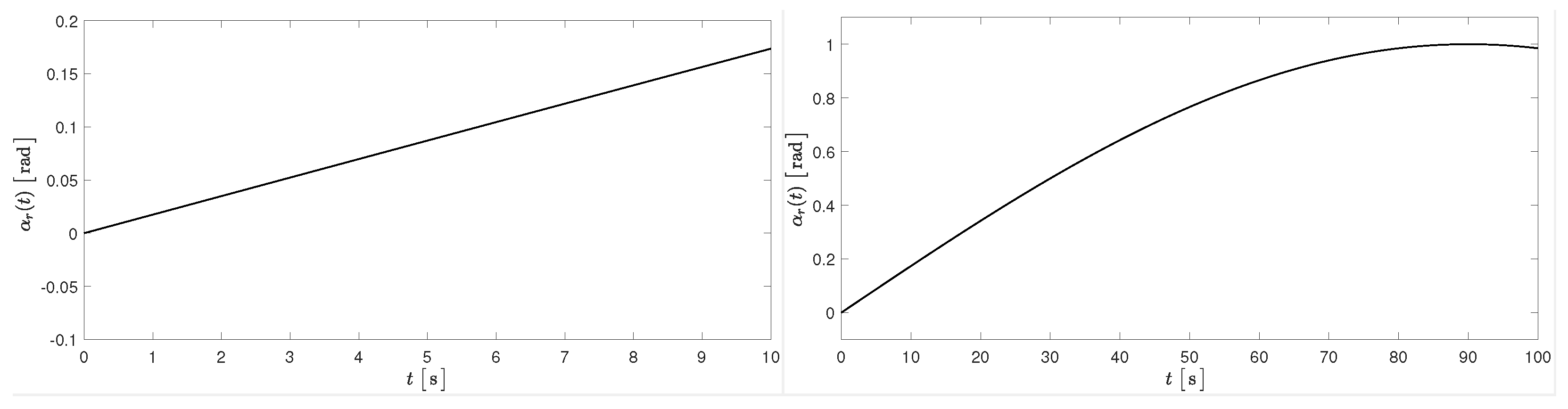
4.1. Reference Signal in Continuous Time

As the continuous-time reference signal has the form ${\displaystyle {\alpha }_r(t)=asin({\omega }_{r}t)}$, it can be generated by a dynamical system ${\displaystyle {\mathsf{\Sigma }}_S}$ (referred to as the exosystem), given as follows:

$${\mathsf{\Sigma }}_S:\left\{\begin{array}{cccc}{\dot{r}}_1(t)& =& r_2(t),\hfill & r_1(0)=0,\hfill \\ {\dot{r}}_2(t)& =& -{\omega }_r^2{r}_1(t),\hfill & r_2(0)=a{\omega }_r,\hfill \\ {\alpha }_r(t)& =& r_1(t),\hfill \end{array}\right.$$

(60)

where ${\displaystyle {\omega }_r>0}$ must be known and ${\displaystyle a\in \mathbb{R}}$ may be unknown. Introducing

${\displaystyle r(t):=\left[\begin{array}{c}{r}_1(t)\\ r_2(t)\end{array}\right]}$, we obtain the following:

$${\mathsf{\Sigma }}_S:\left\{\begin{array}{ccc}\dot{r}(t)& =& Sr(t),r(0)=r_0,\hfill \\ {\alpha }_r(t)& =& Tr(t),\hfill \end{array}\right.$$

(61)

with the state space matrix

$$\left[\begin{array}{c}S\\ T\end{array}\right]=\left[\begin{array}{cc}0& 1\\ -{\omega }_r^2& 0\\ 1& 0\end{array}\right].$$

(62)

The characteristic polynomial of ${\displaystyle S}$ is given as follows:

$$det(\lambda I-S)={\lambda }^2+{\omega }_r^2,$$

(63)

with the spectrum (eigenvalues)

$$\sigma (S)=\{j{\omega }_r;-j{\omega }_r\}\subset j\mathbb{R}.$$

(64)

The pair ${\displaystyle (T,S)}$ is observable, as the observability matrix ${\displaystyle V_S}$ of ${\displaystyle {\mathsf{\Sigma }}_S}$ satisfies the following:

$$det{V}_S=det(\left[\begin{array}{c}T\\ TS\end{array}\right])=1\ne 0.$$

(65)

4.2. The Discrete-Time State Space Model of the Exosystem and Its Properties

We follow the idea of Section 3.2 for the discrete time:

$$t=ih,i\in \mathbb{N},$$

(66)

where ${\displaystyle h>0}$ is the discrete-time step. We integrate over the intervals ${\displaystyle (ih,(i+1)h)}$ on both sides of the state space model (61) and obtain the following:

$$\begin{array}{ccc}\hfill {\int }_{ih}^{(i+1)h}\dot{r}(t)\mathrm{d}t& =& S{\int }_{ih}^{(i+1)h}r(t)\mathrm{d}t,\hfill \\ \hfill {\int }_{ih}^{(i+1)h}{\alpha }_r(t)\mathrm{d}t& =& T{\int }_{ih}^{(i+1)h}r(t)\mathrm{d}t,i\in \mathbb{N}.\hfill \end{array}$$

(67)

Approximating the state integral, according to the mid-point rule, and the integral of the output as before; that is,

$${\int }_{ih}^{(i+1)}r(t)\mathrm{d}t\approx {\displaystyle \frac{h}{2}}(r(ih)+r((i+1)h)),{\int }_{ih}^{(i+1)}{\alpha }_r(t)\mathrm{d}t\approx \sqrt{h}{\alpha }_r^d(ih),$$

(68)

we can rewrite (67) as follows:

$$\begin{array}{ccc}\hfill r^d((i+1)h)-r^d(ih)& =& {\displaystyle \frac{h}{2}}S(r^d(ih)+r^d((i+1)h)),\hfill \\ \hfill \sqrt{h}{\alpha }_r^d(ih)& =& {\displaystyle \frac{h}{2}}T(r^d(ih)+r^d((i+1)h)).\hfill \end{array}$$

(69)

As the matrix ${\displaystyle S}$ satisfies

$$\sigma (S)\subset j\mathbb{R},$$

(70)

then, for all ${\displaystyle h>0}$, the parameter ${\displaystyle \mu }$ satisfies ${\displaystyle \mu >0}$ and

$$\mu ={\displaystyle \frac{2}{h}}\notin \sigma (S).$$

(71)

This implies that there exists an inverse matrix ${\displaystyle {(\mu I-S)}^{-1}}$. Through simple manipulations, (69) can be transformed to the following final form of the discrete-time state space model ${\displaystyle {\mathsf{\Sigma }}_S^d}$ of the exosystem:

$${\mathsf{\Sigma }}_S^d:\left\{\begin{array}{ccc}\hfill r^d(i+1)& =& S^d(\mu )r^d(i),r^d(0)=r(0)=r_0,\hfill \\ \hfill {\alpha }_r^d(i)& =& T^d(\mu )r^d(i),\hfill \end{array}\right.$$

(72)

where

$$\begin{array}{ccc}{S}^d(\mu )& :=& {(\mu I-S)}^{-1}(\mu I+S),\hfill \\ T_d(\mu )& :=& \sqrt{2\mu }T{(\mu I-S)}^{-1},\hfill \end{array}$$

(73)

and we have dropped ${\displaystyle h}$ in order to simplify the notation for ${\displaystyle r^d(ih)}$ and ${\displaystyle {\alpha }_r^d(ih)}$. By repeating the same considerations as in Section 3.3, we see that, for ${\displaystyle \lambda \in \mathbb{C}\setminus \{-1\}}$,

$${\displaystyle \frac{1}{\lambda +1}}det(\lambda I-S^d)det(\mu I-S)=det(\mu {\displaystyle \frac{\lambda -1}{\lambda +1}}I-S),$$

(74)

and as ${\displaystyle det(\mu I-S)\ne 0}$, we have

$$det(\lambda I-S^d)=0\mathrm{if}\mathrm{and}\mathrm{only}\mathrm{if}det(\mu {\displaystyle \frac{\lambda -1}{\lambda +1}}I-S)=0.$$

(75)

If ${\displaystyle -1\notin \sigma (S^d)}$, then the eigenvalues ${\displaystyle {({\lambda }_l(S^d))}_{l=1}^{l=2}}$ and ${\displaystyle {({\mu }_l(S))}_{l=1}^{l=2}}$ are related to each other by the following equality:

$${\mu }_l(S)=\mu {\displaystyle \frac{{\lambda }_l(S^d)-1}{{\lambda }_l(S^d)+1}},l=1,2;$$

(76)

or, equivalently, if ${\displaystyle {\mu }_l(S)\ne \mu }$ (which is always satisfied based on (71)), then

$${\lambda }_l(S^d)={\displaystyle \frac{\mu +{\mu }_l(S)}{\mu -{\mu }_l(S)}},l=1,2.$$

(77)

Therefore,

$$\begin{array}{c}|{\lambda }_l(S^d)|=1\mathrm{if}\mathrm{and}\mathrm{only}\mathrm{if}\mathrm{Re}{\mu }_l(S)=0.\hfill \end{array}$$

(78)

The same considerations as in Section 3.3 demonstrate that the observability of the pair ${\displaystyle (T,S)}$ is equivalent to the observability of ${\displaystyle (T^d,S^d)}$.

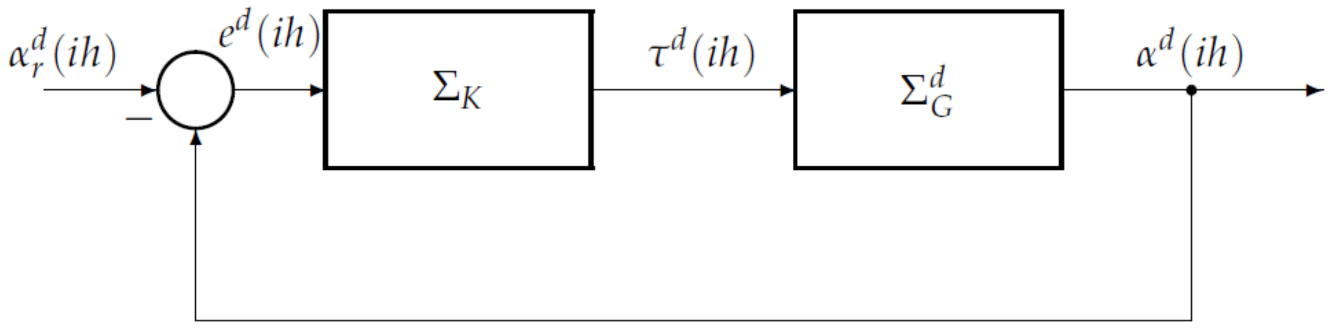
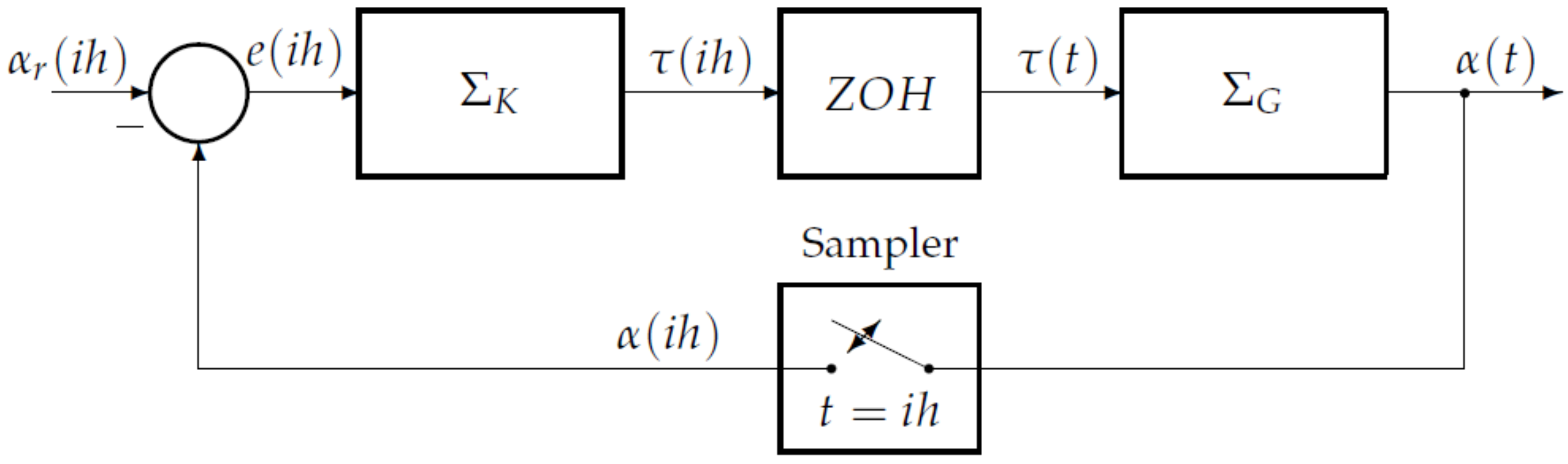
4.3. The Discrete-Time Error Feedback Control System ${\displaystyle {\mathsf{\Sigma }}_{efcs}}$

We are ready to carry out the design of a discrete-time error feedback system. Let us recall the main equations describing the systems in discrete-time (see (27), (9), (6) and (72)); that is, the discrete-time plant:

$${\mathsf{\Sigma }}_G^d:\left\{\begin{array}{ccc}\hfill x^d(i+1)& =& A^d(\mu )x^d(i)+B^d(\mu ){\tau }^d(i),x^d(0)=x(0)=x_0,\hfill \\ \hfill {\alpha }^d(i)& =& C^d(\mu )x^d(i)+D^d(\mu ){\tau }^d(i),\hfill \end{array}\right.$$

(79)

the discrete-time controller:

$${\mathsf{\Sigma }}_K:\left\{\begin{array}{ccc}\hfill x_K(i+1)& =& A_K{x}_K(i)+B_K{e}^d(i),x_K(0)=x_{K0},\hfill \\ \hfill {\tau }^d(i)& =& C_K{x}_K(i),\hfill \end{array}\right.$$

(80)

the discrete-time error:

$$e^d(i)={\alpha }^d(i)-{\alpha }_r^d(i),i\in \mathbb{N}$$

(81)

and the discrete-time exosystem:

$${\mathsf{\Sigma }}_S^d:\left\{\begin{array}{ccc}\hfill r^d(i+1)& =& S^d(\mu )r^d(i),r^d(0)=r(0)=r_0,\hfill \\ \hfill {\alpha }_r^d(i)& =& T^d(\mu )r^d(i).\hfill \end{array}\right.$$

(82)

In order to simplify the notation, we drop ${\displaystyle \mu }$ in all system matrices.

Combining (79)–(81), we obtain the basic model of the discrete-time error feedback control system (see Figure 2), denoted by ${\displaystyle {\mathsf{\Sigma }}_{efcs}}$, with ${\displaystyle {({\alpha }_r^d(i))}_{i\in \mathbb{N}}}$ as an external reference signal. Its model takes the following form:

$${\mathsf{\Sigma }}_{efcs}:\left\{\begin{array}{ccc}{x}^d(i+1)& =& A^d{x}^d(i)+B^d{C}_K{x}_K(i),x^d(0)=x_0,\hfill \\ x_K(i+1)& =& B_K{C}^d{x}^d(i)+(A_K+B_K{D}^d{C}_K)x_K(i)-B_K{\alpha }_r^d(i),x_K(0)=x_{K0},\hfill \\ e^d(i)& =& C^d{x}^d(i)+D^d{C}_K{x}_K(i)-{\alpha }_r^d(i).\hfill \end{array}\right.$$

(83)

The error feedback control system ${\displaystyle {\mathsf{\Sigma }}_{efcs}}$ with zero input (i.e., ${\displaystyle {\alpha }_r^d\equiv 0}$) and without the output equation is referred to as the discrete-time unforced closed loop system ${\displaystyle {\mathsf{\Sigma }}_{uf}}$, and its description simplifies to the following autonomous form:

$${\mathsf{\Sigma }}_{uf}:\left[\begin{array}{c}{x}^d(i+1)\\ x_K(i+1)\end{array}\right]=\left[\begin{array}{cc}{A}^d& B^d{C}_K\\ B_K{C}^d& A_K+B_K{D}^d{C}_K\end{array}\right]\left[\begin{array}{c}{x}^d(i)\\ x_K(i)\end{array}\right],\left[\begin{array}{c}{x}^d(0)\\ x_K(0)\end{array}\right]=\left[\begin{array}{c}{x}_0\\ x_{K0}\end{array}\right].$$

(84)

If we take into account the fact that the reference ${\displaystyle {\alpha }_r^d(i)}$ is generated by the discrete-time exosystem ${\displaystyle {\mathsf{\Sigma }}_S^d}$ and combine equations (83) and (82), then we obtain the following discrete-time forced closed loop system ${\displaystyle {\mathsf{\Sigma }}_{cl}}$:

$${\mathsf{\Sigma }}_{cl}:\left\{\begin{array}{ccc}{x}^d(i+1)& =& A^d{x}^d(i)+B^d{C}_K{x}_K(i),x^d(0)=x_0,\hfill \\ x_K(i+1)& =& (A_K+B_K{D}^d{C}_K)x_K(i)+B_K{C}^d{x}^d(i)-B_K{T}^d{r}^d(i),x_K(0)=x_{K0},\hfill \\ r^d(i+1)& =& S^d{r}^d(i),r^d(0)=r_0,\hfill \\ e^d(i)& =& C^d{x}^d(i)+D^d{C}_K{x}_K(i)-T^d{r}^d(i).\hfill \end{array}\right.$$

(85)

Now, we are ready to precisely define—in mathematical terms—the error feedback controller that we are looking for. We require the controller (80) to guarantee that the following two conditions hold:

IS:

Internal stability. The error feedback control system ${\displaystyle {\mathsf{\Sigma }}_{efcs}}$ is said to be internally stable if the unforced closed system ${\displaystyle {\mathsf{\Sigma }}_{uf}}$ is asymptotically stable; that is, for all ${\displaystyle x^d(0)=x_0}$, ${\displaystyle x_K(0)=x_{K0}}$, we have the following:

$$\underset{i\to \infty }{lim}\left[\begin{array}{c}{x}^d(i)\\ x_K(i)\end{array}\right]=0.$$

(86)

AT:

Asymptotic tracking (or regulation). The error feedback control system ${\displaystyle {\mathsf{\Sigma }}_{efcs}}$ is said to satisfy the asymptotic tracking condition if, for all ${\displaystyle r^d(0)=r_0}$, ${\displaystyle x^d(0)=x_0}$, and ${\displaystyle x_K(0)=x_{K0}}$, the forced closed loop system ${\displaystyle {\mathsf{\Sigma }}_{cl}}$ satisfies the following:

$$\underset{i\to \infty }{lim}{e}^d(i)=0.$$

It can be seen from (84) that IS holds if and only if

$$\sigma (\left[\begin{array}{cc}{A}^d& B^d{C}_K\\ B_K{C}^d& A_K+B_K{D}^d{C}_K\end{array}\right])\subset {\mathbb{D}}_1,$$

(87)

where ${\displaystyle {\mathbb{D}}_1}$ denotes the open unit disk ${\displaystyle {\mathbb{D}}_1:=\{z\in \mathbb{C}:|z|<1\}}$. In turn, AT requires further study.

Before we proceed with the general error feedback controller ${\displaystyle {\mathsf{\Sigma }}_K}$, it is convenient to start with a simple static state feedback case, which is described in the next subsection.

4.4. Static State Feedback for the Extended Discrete-Time Plant

We start with a simple situation, which turns out to be useful in our later considerations. Combining (79), (82), and (81), we introduce the so-called extended discrete-time plant ${\displaystyle {\mathsf{\Sigma }}_{ext}}$, defined as follows:

$${\mathsf{\Sigma }}_{ext}:\left\{\begin{array}{ccc}{x}^d(i+1)& =& A^d{x}^d(i)+B^d{\tau }^d(i),x^d(0)=x_0,\hfill \\ r^d(i+1)& =& S^d{r}^d(i),r^d(0)=r_0,\hfill \\ e^d(i)& =& C^d{x}^D(i)-T^d{r}^d(i)+D^d{\tau }^d(i).\hfill \end{array}\right.$$

(88)

As detailed above, the transformation from ${\displaystyle (A,B,C,0)}$ to ${\displaystyle (A^d,B^d,C^d,D^d)}$ preserves controllability and observability, and the transformation from ${\displaystyle (S,T)}$ to ${\displaystyle (S^d,T^d)}$ also preserves observability. Therefore, as ${\displaystyle (A,B)}$ is controllable, so is ${\displaystyle (A^d,B^d)}$; and as ${\displaystyle (C,A)}$ and ${\displaystyle (T,S)}$ are observable, so are ${\displaystyle (C^d,A^d)}$ and ${\displaystyle (T^d,S^d)}$. It is well-known (see, e.g., [22]) that, under the above conditions, there always exists a feedback gain matrix ${\displaystyle F\in {\mathbb{R}}^{1\times 4}}$ such that ${\displaystyle \sigma (A^d-B^{d}F)\subset {\mathbb{D}}_1}$. If we insert the static state feedback

$${\tau }^d(i)=-F{x}^d(i)+Q{r}^d(i),i\in \mathbb{N},$$

(89)

then we get the following closed loop system ${\displaystyle {\mathsf{\Sigma }}_{cl}^0}$:

$${\mathsf{\Sigma }}_{cl}^0:\left\{\begin{array}{ccc}{x}^d(i+1)& =& (A^d-B^{d}F)x^d(i)+B^{d}Q{r}^d(i),x^d(0)=x_0,\hfill \\ r^d(i+1)& =& S^d{r}^d(i),r^d(0)=r_0,\hfill \\ e^d(i)& =& (C^d-D^{d}F)x^d(i)+(D^{d}Q-T^d)r^d(i).\hfill \end{array}\right.$$

(90)

Theorem 1.

If ${\displaystyle b>0}$ or ${\displaystyle b=0}$ and ${\displaystyle k\ne {\omega }_r^{2}p}$, then there exists a static state feedback controller (89) such that, for ${\displaystyle {\mathsf{\Sigma }}_{cl}^0}$, we have the following:

$$\underset{i\to \infty }{lim}{e}^d(i)=0.$$

(91)

One such controller is given by the following formula:

$${\tau }^d(i)=\left[\begin{array}{cc}-F& \mathsf{\Gamma }+F\mathsf{\Pi }\end{array}\right]\left[\begin{array}{c}{x}^d(i)\\ r^d(i)\end{array}\right],$$

(92)

where ${\displaystyle F\in {\mathbb{R}}^{1\times 4}}$ is such that ${\displaystyle \sigma (A^d-B^{d}F)\subset {\mathbb{D}}_1}$ and the pair of matrices ${\displaystyle (\mathsf{\Pi },\mathsf{\Gamma })}$, where ${\displaystyle \mathsf{\Pi }\in {\mathbb{R}}^{4\times 2}}$ and ${\displaystyle \mathsf{\Gamma }\in {\mathbb{R}}^{1\times 2}}$ is a unique solution of the matrix regulator equation:

$$\left\{\begin{array}{c}{A}^d\mathsf{\Pi }-\mathsf{\Pi }{S}^d+B^d\mathsf{\Gamma }=0,\hfill \\ C^d\mathsf{\Pi }-T^d+D^d\mathsf{\Gamma }=0.\hfill \end{array}\right.$$

(93)

Proof. 

Assume ${\displaystyle F}$ such that ${\displaystyle \sigma (A^d-B^{d}F)\subset {\mathbb{D}}_1}$ and let ${\displaystyle Q\in {\mathbb{R}}^{1\times 2}}$ be arbitrary. We start with the equivalent state variables:

$$\left[\begin{array}{c}{p}^d(i)\\ r^d(i)\end{array}\right]=\left[\begin{array}{cc}I& -\mathsf{\Pi }\\ 0& I\end{array}\right]\left[\begin{array}{c}{x}^d(i)\\ r^d(i)\end{array}\right],i\in \mathbb{N},$$

(94)

where ${\displaystyle \mathsf{\Pi }\in {\mathbb{R}}^{4\times 2}}$ can be arbitrary. From (94) and (90), we easily get

$$\begin{array}{ccc}{p}^d(i+1)& =& x^d(i+1)-\mathsf{\Pi }{r}^d(i+1)\hfill \\ & =& (A^d-B^{d}F)x^d(i)+B^{d}Q{r}^d(i)-\mathsf{\Pi }{S}^d{r}^d(i)\hfill \\ & =& (A^d-B^{d}F)p^d(i)+((A^d-B^{d}F)\mathsf{\Pi }-\mathsf{\Pi }{S}^d+B^{d}Q)r^d(i),\hfill \\ e^d(i)& =& (C^d-D^{d}F)p^d(i)+((C^d-D^{d}F)\mathsf{\Pi }-T^d+D^{d}Q))r^d(i)\hfill \end{array}$$

(95)

and, if the matrix equation

$$\left\{\begin{array}{c}(A^d-B^{d}F)\mathsf{\Pi }-\mathsf{\Pi }{S}^d+B^{d}Q=0,\hfill \\ (C^d-D^{d}F)\mathsf{\Pi }-T^d+D^{d}Q=0,\hfill \end{array}\right.$$

(96)

has a solution ${\displaystyle (\mathsf{\Pi },Q)}$, then (95) implies

$$\begin{array}{cccc}{p}^d(i+1)& =& (A^d-B^{d}F)p^d(i),\hfill & p^d(0)=x_0-\mathsf{\Pi }{r}_0,\hfill \\ e^d(i)& =& (C^d-D^{d}F)p^d(i).\hfill \end{array}$$

(97)

As ${\displaystyle \sigma (A^d-B^{d}F)\subset {\mathbb{D}}_1}$, then for any initial states ${\displaystyle x^d(0)=x_0}$ and ${\displaystyle r^d(0)=r_0}$, we get

$$\underset{i\to \infty }{lim}{p}^d(i)=\underset{i\to \infty }{lim}({(A^d-B^{d}F)}^i(x_0-\mathsf{\Pi }{r}_0)=0$$

(98)

and, hence, ${\displaystyle \underset{i\to \infty }{lim}{e}^d(i)=0}$ (i.e., (91) holds).

On the other hand, as ${\displaystyle \sigma (S^d)\subset \mathbb{C}\setminus {\mathbb{D}}_1}$, then ${\displaystyle \sigma (S^d)\cap \sigma (A^d-B^{d}F)=\oslash }$ and, for any matrix ${\displaystyle Q}$, the Sylvester equation

$$(A^d-B^{d}F)\mathsf{\Pi }-\mathsf{\Pi }{S}^d+B^{d}Q=0$$

(99)

has a unique solution ${\displaystyle \mathsf{\Pi }}$. Now, it follows from (95) that

$$\begin{array}{ccc}{p}^d(i+1)& =& (A^d-B^{d}F)p^d(i),p^d(0)=x_0-\mathsf{\Pi }{r}_0,\hfill \\ e^d(i)& =& (C^d-D^{d}F)p^d(i)+((C^d-D^{d}F)\mathsf{\Pi }-T^d+D^{d}Q)r^d(i).\hfill \end{array}$$

(100)

Moreover, for any ${\displaystyle x^d(0)=x_0}$ and ${\displaystyle r^d(0)=r_0}$, we have ${\displaystyle \underset{i\to \infty }{lim}{p}^d(i)=0}$ and, based on (91), we also have ${\displaystyle \underset{i\to \infty }{lim}{e}^d(i)=0}$. Thus, for any initial state ${\displaystyle r^d(0)=r_0}$, we obtain the following:

$$\underset{i\to \infty }{lim}((C^d-D^{d}F)\mathsf{\Pi }-T^d+D^{d}Q)r^d(i)=\underset{i\to \infty }{lim}((C^d-D^{d}F)\mathsf{\Pi }-T^d+D^{d}Q){(S^d)}^i{r}_0=0.$$

(101)

As ${\displaystyle \sigma (S^d)\subset \mathbb{C}\setminus {\mathbb{D}}_1}$, then (101) implies ${\displaystyle (C^d-D^{d}F)\mathsf{\Pi }-T^d+D^{d}Q=0}$ for ${\displaystyle \mathsf{\Pi }}$ from (99).

Finally, let us note that the matrix Equation (96) can be written as follows:

$$\left\{\begin{array}{c}{A}^d\mathsf{\Pi }-\mathsf{\Pi }{S}^d+B^d(Q-F\mathsf{\Pi })=0,\hfill \\ C^d\mathsf{\Pi }-T^d+D^d(Q-F\mathsf{\Pi })=0\hfill \end{array}\right.$$

(102)

which, after the substitution ${\displaystyle \mathsf{\Gamma }=Q-F\mathsf{\Pi }}$, takes the form of the regulator Equation (93).

The results we have proved above are a direct extension of the continuous-time general regulation theory (see, e.g., [14]) to the discrete-time scenario. However, an important question now arises regarding if and when the regulator Equation (93) admits a solution in terms of the physical parameters ${\displaystyle I}$, ${\displaystyle p}$, ${\displaystyle k}$, ${\displaystyle b}$, and ${\displaystyle {\omega }_r}$. From Section 3.3, we know that ${\displaystyle D^d=C{(\mu I-A)}^{-1}B}$ is invertible, which allows us to express ${\displaystyle \mathsf{\Gamma }}$ in the following form:

$$\mathsf{\Gamma }=-{(D^d)}^{-1}{C}^d\mathsf{\Pi }+{(D^d)}^{-1}{T}^d,$$

(103)

and then to transform the first equation in (93) to the standard Sylvester matrix equation:

$$(A^d-B^d{(D^d)}^{-1}{C}^d)\mathsf{\Pi }-\mathsf{\Pi }{S}^d+B^d{(D^d)}^{-1}{T}^d=0.$$

(104)

As the existence of a solution ${\displaystyle (\mathsf{\Pi },\mathsf{\Gamma })}$ to Equation (93) is equivalent to the existence of a solution ${\displaystyle \mathsf{\Pi }}$ to Equation (104), and it is known that the Sylvester equation has a unique solution if and only if

$$\sigma (A^d-B^d{(D^d)}^{-1}{C}^d)\cap \sigma (S^d)=\oslash ,$$

(105)

then under Condition (105), the regulator equation also has a unique solution ${\displaystyle (\mathsf{\Pi },\mathsf{\Gamma })}$, where ${\displaystyle \mathsf{\Pi }}$ is a solution to (104) and ${\displaystyle \mathsf{\Gamma }}$ is given by (103).

We know from Section 3.3, the spectrum ${\displaystyle \sigma (A^d-B^d{(D^d)}^{-1}{C}^d)}$ coincides with the zeros of the system ${\displaystyle {\mathsf{\Sigma }}_G^d}$. Hence, the regulator equation has a (unique) solution ${\displaystyle (\mathsf{\Pi },\mathsf{\Gamma })}$ if and only if the spectrum ${\displaystyle \sigma (S^d)}$ is disjoint with the set of zeros of the system ${\displaystyle {\mathsf{\Sigma }}_G^d}$. In order to show that this is the case for our system, we use the expressions (77), (64), (55), and (18); namely,

$${\lambda }_1(S^d)={\displaystyle \frac{\mu +j{\omega }_r}{\mu -j{\omega }_r}},{\lambda }_2(S^d)={\displaystyle \frac{\mu -j{\omega }_r}{\mu +j{\omega }_r}},$$

(106)

and

$$z_l({\mathsf{\Sigma }}_G^d)={\displaystyle \frac{\mu +s_l({\mathsf{\Sigma }}_G)}{\mu -s_l({\mathsf{\Sigma }}_G)}},l=1,2,$$

(107)

where

$$s_1({\mathsf{\Sigma }}_G)=-{\displaystyle \frac{b}{2p}}-\sqrt{{\left({\displaystyle \frac{b}{2p}}\right)}^2-{\displaystyle \frac{k}{p}}},s_2({\mathsf{\Sigma }}_G)=-{\displaystyle \frac{b}{2p}}+\sqrt{{\left({\displaystyle \frac{b}{2p}}\right)}^2-{\displaystyle \frac{k}{p}}}.$$

(108)

Simple considerations show that, if ${\displaystyle b>0}$, then ${\displaystyle {({\lambda }_l(S^d))}_{l=1}^{l=2}\cap {(z_l({\mathsf{\Sigma }}_G^d))}_{l=1}^{l=2}=\oslash }$; meanwhile, for ${\displaystyle b=0}$, the latter condition still holds if and only if ${\displaystyle k\ne {\omega }_r^{2}p}$. ${\displaystyle \square }$

Theorem 1 is essential, as it provides a basis for the development of the dynamic error feedback controller in the form of (80).

4.5. Characterization of the Discrete-Time Error Feedback Controller

If we interconnect the extended discrete-time plant ${\displaystyle {\mathsf{\Sigma }}_{ext}}$, defined in the following form:

$${\mathsf{\Sigma }}_{ext}:\left\{\begin{array}{ccc}{x}^d(i+1)& =& A^d{x}^d(i)+B^d{\tau }^d(i),x^d(0)=x_0,\hfill \\ r^d(i+1)& =& S^d{r}^d(i),r^d(0)=r_0,\hfill \\ e^d(i)& =& C^d{x}^d(i)-T^d{r}^d(i)+D^d{\tau }^d(i),\hfill \end{array}\right.$$

(109)

and the discrete-time controller:

$${\mathsf{\Sigma }}_K:\left\{\begin{array}{ccc}\hfill x_K(i+1)& =& A_K{x}_K(i)+B_K{e}^d(i),x_K(0)=x_{K0},\hfill \\ \hfill {\tau }^d(i)& =& C_K{x}_K(i),\hfill \end{array}\right.$$

(110)

then we obtain the discrete-time forced closed loop system  ${\displaystyle {\mathsf{\Sigma }}_{cl}}$:

$${\mathsf{\Sigma }}_{cl}:\left\{\begin{array}{ccc}{x}^d(i+1)& =& A^d{x}^d(i)+B^d{C}_K{x}_K(i),x^d(0)=x_0,\hfill \\ x_K(i+1)& =& (A_K+B_K{D}^d{C}_K)x_K(i)+B_K{C}^d{x}^d(i)-B_K{T}^d{r}^d(i),x_K(0)=x_{K0},\hfill \\ r^d(i+1)& =& S^d{r}^d(i),r^d(0)=r_0,\hfill \\ e^d(i)& =& C^d{x}^d(i)+D^d{C}_K{x}_K(i)-T^d{r}^d(i).\hfill \end{array}\right.$$

(111)

As we already know, IS holds if and only if

$$\sigma (\left[\begin{array}{cc}{A}^d& B^d{C}_K\\ B_K{C}^d& A_K+B_K{D}^d{C}_K\end{array}\right])\subset {\mathbb{D}}_1.$$

(112)

As ${\displaystyle (A^d,B^d)}$ is controllable and ${\displaystyle (C^d,A^d)}$ is observable, there always exists a controller ${\displaystyle (A_K,B_K,C_K,0)}$ satisfying (112). In the continuous-time case, for a controller satisfying IS, the general regulation theory (see, e.g., [14]) provides necessary and sufficient conditions to be satisfied for the asymptotic tracking condition AT to hold. We extend these results to the discrete-time case and, in order to keep our exposition complete, we provide the corresponding results with proofs.

Theorem 2.

If, for a given controller ${\displaystyle (A_K,B_K,C_K,0)}$, the condition IS holds, then the closed loop system ${\displaystyle {\mathsf{\Sigma }}_{cl}}$ satisfies the asymptotic tracking condition AT if and only if there exist ${\displaystyle \mathsf{\Pi }\in {\mathbb{R}}^{4\times 2}}$, ${\displaystyle \mathsf{\Gamma }\in {\mathbb{R}}^{1\times 2}}$, and ${\displaystyle \mathsf{\Sigma }\in {\mathbb{R}}^{n_K\times 2}}$ such that

$$\mathrm{R}\mathrm{E}:\left\{\begin{array}{c}{A}^d\mathsf{\Pi }-\mathsf{\Pi }{S}^d+B^d\mathsf{\Gamma }=0,\hfill \\ C^d\mathsf{\Pi }-T^d+D^d\mathsf{\Gamma }=0,\hfill \end{array}\right.$$

(113)

and

$$\mathrm{I}\mathrm{M}\mathrm{P}:\left\{\begin{array}{c}\mathsf{\Gamma }=C_K\mathsf{\Sigma },\hfill \\ \mathsf{\Sigma }{S}^d=A_K\mathsf{\Sigma }.\hfill \end{array}\right.$$

(114)

Proof. 

Let (112) hold. For the closed-loop system (111), we introduce new state variables:

$$\left[\begin{array}{c}{p}^d(i)\\ q^d(i)\\ r^d(i)\end{array}\right]=\left[\begin{array}{ccc}I& 0& -\mathsf{\Pi }\\ 0& I& -\mathsf{\Sigma }\\ 0& 0& I\end{array}\right]\left[\begin{array}{c}{x}^d(i)\\ x_K(i)\\ r^d(i)\end{array}\right],$$

(115)

where ${\displaystyle \mathsf{\Pi }\in {\mathbb{R}}^{4\times 2}}$ and ${\displaystyle \mathsf{\Sigma }\in {\mathbb{R}}^{n_K\times 2}}$ can be arbitrary, and we obtain the following:

$${\mathsf{\Sigma }}_{cl}:\left\{\begin{array}{ccc}\hfill p^d(i+1)& =& A^d{p}^d(i)+B^d{C}_K{q}^d(i)+(A^d\mathsf{\Pi }-\mathsf{\Pi }{S}^d+B^d{C}_K\mathsf{\Sigma })r^d(i),\hfill \\ \hfill & & p^d(0)=x_0-\mathsf{\Pi }{r}_0,\hfill \\ \hfill q^d(i+1)& =& B_K{C}^d{p}^d(i)+(A_K+B_K{D}^d{C}_K)q^d(i)\hfill \\ \hfill & & +[(A_K+B_K{D}^d{C}_K)\mathsf{\Sigma }-\mathsf{\Sigma }{S}^d+B_K(C^d\mathsf{\Pi }-T^d)]r^d(i),\hfill \\ \hfill & & q^d(0)=x_{K0}-\mathsf{\Sigma }{r}_0,\hfill \\ \hfill r^d(i+1)& =& S^d{r}^d(i),r^d(0)=r_0,\hfill \\ \hfill e^d(i)& =& C^d{p}^d(i)+D^d{C}_K{q}^d(i)+(C^d\mathsf{\Pi }-T^d+D^d{C}_K\mathsf{\Sigma })r^d(i).\hfill \end{array}\right.$$

(116)

If there exist matrices ${\displaystyle (\mathsf{\Pi },\mathsf{\Sigma })}$ such that

$$\left[\begin{array}{cc}{A}^d& B^d{C}_K\\ B_K{C}^d& A_K+B_K{D}^d{C}_K\end{array}\right]\left[\begin{array}{c}\mathsf{\Pi }\\ \mathsf{\Sigma }\end{array}\right]-\left[\begin{array}{c}\mathsf{\Pi }\\ \mathsf{\Sigma }\end{array}\right]S^d=\left[\begin{array}{c}0\\ B_K{T}^d\end{array}\right],$$

(117)

and

$$C^d\mathsf{\Pi }-T^d+D^d{C}_K\mathsf{\Sigma }=0,$$

(118)

then (116) simplifies to the following form:

$${\mathsf{\Sigma }}_{cl}:\left[\begin{array}{c}{p}^d(i+1)\\ q^d(i+1)\\ r^d(i+1)\\ e^d(i)\end{array}\right]=\left[\begin{array}{ccc}{A}^d& B^d{C}_K& \\ B_K{C}^d& A_K+B_K{D}^d{C}_K& 0\\ 0& 0& S^d\\ C^d& D^d{C}_K& 0\end{array}\right]\left[\begin{array}{c}{p}^d(i)\\ q^d(i)\\ r^d(i)\end{array}\right].$$

(119)

Due to (112), this implies that

$$\begin{array}{c}{\displaystyle \underset{i\to \infty }{lim}}{e}^d(i)={\displaystyle \underset{i\to \infty }{lim}}\left[\begin{array}{cc}{C}^d& D^d{C}_K\end{array}\right]{\left[\begin{array}{cc}{A}^d& B^d{C}_K\\ B_K{C}^d& A_K+B_K{D}^d{C}_K\end{array}\right]}^i\left[\begin{array}{c}{p}^d(0)\\ q^d(0)\end{array}\right]=0;\hfill \end{array}$$

(120)

that is, the asymptotic tracking condition (AT) holds.

On the other hand, as

$$\sigma (\left[\begin{array}{cc}{A}^d& B^d{C}_K\\ B_K{C}^d& A_K+B_K{D}^d{C}_K\end{array}\right])\cap \sigma (S^d)=\oslash ,$$

(121)

then for every ${\displaystyle \left[\begin{array}{c}0\\ B_K{T}^d\end{array}\right]}$ the Sylvester Equation (117) has a unique solution ${\displaystyle \left[\begin{array}{c}\mathsf{\Pi }\\ \mathsf{\Sigma }\end{array}\right]}$. This equation and the asymptotic tracking condition AT, applied to System (116), imply the following:

$$\begin{array}{ccc}\hfill {\displaystyle \underset{i\to \infty }{lim}}{e}^d(i)& =& {\displaystyle \underset{i\to \infty }{lim}}\left[\begin{array}{cc}{C}^d& D^d{C}_K\end{array}\right]{\left[\begin{array}{cc}{A}^d& B^d{C}_K\\ B_K{C}^d& A_K+B_K{D}^d{C}_K\end{array}\right]}^i\left[\begin{array}{c}{x}_0-\mathsf{\Pi }{r}_0\\ x_{K0}-\mathsf{\Sigma }{r}_0\end{array}\right]\hfill \\ \hfill & & +{\displaystyle \underset{i\to \infty }{lim}}(C^d\mathsf{\Pi }-T^d+D^d{C}_K\mathsf{\Sigma }){(S^d)}^i{r}_0\hfill \\ \hfill & =& {\displaystyle \underset{i\to \infty }{lim}}(C^d\mathsf{\Pi }-T^d+D^d{C}_K\mathsf{\Sigma }){(S^d)}^i{r}_0=0.\hfill \end{array}$$

(122)

As ${\displaystyle \sigma (S^d)\cap {\mathbb{D}}_1=\oslash }$, we get ${\displaystyle C^d\mathsf{\Pi }-T^d+D^d{C}_K\mathsf{\Sigma }=0}$.

Now let us note that, by substituting (118) into (117), we get an equivalent set of equations:

$$\left\{\begin{array}{c}{A}^d\mathsf{\Pi }-\mathsf{\Pi }{S}^d+B^d{C}_K\mathsf{\Sigma }=0,\hfill \\ A_K\mathsf{\Sigma }-\mathsf{\Sigma }{S}^d=0,\hfill \\ C^d\mathsf{\Pi }-T^d+D^d{C}_K\mathsf{\Sigma }=0.\hfill \end{array}\right.$$

(123)

Finally, if we introduce ${\displaystyle \mathsf{\Gamma }=C_K\mathsf{\Sigma }}$, then (123) can be equivalently written as (113) and (114). ${\displaystyle \square }$

Relation (113) is the regulator equation from Theorem 1; hence, we denote it as RE. Furthermore, the second relation (114) is called the internal model principle (see, e.g., [14,23]), which we denote as IMP. The latter relation reflects the fact that a sensible controller has to include the dynamics of the exosystem.

In order to develop a controller ${\displaystyle (A_K,B_K,C_K)}$, we turn back to the result of Theorem 1 for the static state feedback controller. However, we assume that only the output of the plant can be measured, so, the components of the extended state ${\displaystyle \left[\begin{array}{c}{x}^d(i)\\ r^d(i)\end{array}\right]}$ are not available for the state feedback. As we can compute the error signal ${\displaystyle e^d(i)}$—that is, the output of the extended plant ${\displaystyle {\mathsf{\Sigma }}_{ext}}$—we can construct a classic full-order asymptotic observer to estimate the extended state and try the approximate state ${\displaystyle \left[\begin{array}{c}{\tilde{x}}^d(i)\\ {\tilde{r}}^d(i)\end{array}\right]}$ in the control law

$${\tau }^d(i)=\left[\begin{array}{cc}-F& \mathsf{\Gamma }+F\mathsf{\Pi }\end{array}\right]\left[\begin{array}{c}{\tilde{x}}^d(i)\\ {\tilde{r}}^d(i)\end{array}\right],i\in \mathbb{N}.$$

(124)

In the next subsection, we show that if the observer is fed the error ${\displaystyle e^d(i)}$, we obtain the required discrete-time error feedback controller (110).

4.6. Derivation of the Discrete-Time Error Feedback Controller Based on a Full-Order Observer

We rewrite the extended plant model ${\displaystyle {\mathsf{\Sigma }}_{ext}}$ (see (109)) in the following form:

$${\mathsf{\Sigma }}_{ext}:\left\{\begin{array}{ccc}\left[\begin{array}{c}{x}^d(i+1)\\ r^d(i+1)\end{array}\right]& =& \left[\begin{array}{cc}{A}^d& 0\\ 0& S^d\end{array}\right]\left[\begin{array}{c}{x}^d(i)\\ r^d(i)\end{array}\right]+\left[\begin{array}{c}{B}^d\\ 0\end{array}\right]{\tau }^d(i),\hfill \\ & & \left[\begin{array}{c}{x}^d(0)\\ r^d(0)\end{array}\right]=\left[\begin{array}{c}{x}_0\\ r_0\end{array}\right],\hfill \\ e^d(i)& =& \left[\begin{array}{cc}{C}^d& -T^d\end{array}\right]\left[\begin{array}{c}{x}^d(i)\\ r^d(i)\end{array}\right]+D^d{\tau }^d(i).\hfill \end{array}\right.$$

(125)

In the research [19], it was shown that, for the pair ${\displaystyle \left(\left[\begin{array}{cc}C& -T\end{array}\right],\left[\begin{array}{cc}A& 0\\ 0& S\end{array}\right]\right),}$ the observability matrix ${\displaystyle V}$ satisfies

$$detV=det\left[\begin{array}{cc}C& -T\\ CA& -TS\\ ⋮& ⋮\\ C{A}^5& -T{S}^5\end{array}\right]=-{\displaystyle \frac{k^2{\omega }_r^2}{I^2}}({\omega }_r^2{\left({\displaystyle \frac{b}{p}}+{\displaystyle \frac{b}{I}}\right)}^2+{\left({\displaystyle \frac{k}{p}}+{\displaystyle \frac{k}{I}}-{\omega }_r^2\right)}^2),$$

(126)

which demonstrates that, for ${\displaystyle b>0}$, the pair is observable; meanwhile, if ${\displaystyle b=0}$, then it is still observable if and only if ${\displaystyle \frac{k}{p}+\frac{k}{I}\ne {\omega }_r^2}$.

As we know from Section 3.3, the observability is preserved under our discretization scheme, and it follows that the same condition also holds for the following pair: ${\displaystyle \left(\left[\begin{array}{cc}{C}^d& -T^d\end{array}\right],\left[\begin{array}{cc}{A}^d& 0\\ 0& S^d\end{array}\right]\right)}$. More precisely, if ${\displaystyle b>0}$ or ${\displaystyle b=0}$ and ${\displaystyle \frac{k}{p}+\frac{k}{I}\ne {\omega }_r^2}$, then the plant ${\displaystyle {\mathsf{\Sigma }}_{ext}}$ is observable. It is a classic result (see, e.g., [22,24]) that, in this case, the asymptotic full-order state observer for ${\displaystyle {\mathsf{\Sigma }}_{ext}}$ exists and has the following form:

$$\begin{array}{ccc}\hfill {\mathsf{\Sigma }}_O:\left[\begin{array}{c}{\tilde{x}}^d(i+1)\\ {\tilde{r}}^d(i+1)\end{array}\right]& =& \left(\left[\begin{array}{cc}{A}^d& 0\\ 0& S^d\end{array}\right]-\left[\begin{array}{c}{L}_1\\ L_2\end{array}\right]\left[\begin{array}{cc}{C}^d& -T^d\end{array}\right]\right)\left[\begin{array}{c}{\tilde{x}}^d(i)\\ {\tilde{r}}^d(i)\end{array}\right]\hfill \\ \hfill & & +\left[\begin{array}{c}{B}^d\\ 0\end{array}\right]{\tau }^d(i)+\left[\begin{array}{c}{L}_1\\ L_2\end{array}\right]e^d(i),\hfill \end{array}$$

(127)

where ${\displaystyle \left[\begin{array}{c}{L}_1\\ L_2\end{array}\right]\in {\mathbb{R}}^{6\times 1}}$ satisfies

$$\sigma (\left[\begin{array}{cc}{A}^d& 0\\ 0& S^d\end{array}\right]-\left[\begin{array}{c}{L}_1\\ L_2\end{array}\right]\left[\begin{array}{cc}{C}^d& -T^d\end{array}\right])=\sigma (\left[\begin{array}{cc}{A}^d-L_1{C}^d& L_1{T}^d\\ -L_2{C}^d& S^d+L_2{T}^d\end{array}\right])\subset {\mathbb{D}}_1,$$

(128)

and this spectrum can be freely assigned.

We have also proven that, for ${\displaystyle b>0}$ or ${\displaystyle b=0}$ and ${\displaystyle k\ne {\omega }_r^{2}p}$, the regulator equation RE has a unique solution ${\displaystyle (\mathsf{\Pi },\mathsf{\Gamma })}$.

In summary, if ${\displaystyle b>0}$ or ${\displaystyle b=0}$ and ${\displaystyle \frac{k}{p}\ne {\omega }_r^2}$, together with ${\displaystyle \frac{k}{I}+\frac{k}{p}\ne {\omega }_r^2}$, then we can make use of the control law

$${\tau }^d(i)=\left[\begin{array}{cc}-F& \mathsf{\Gamma }+F\mathsf{\Pi }\end{array}\right]\left[\begin{array}{c}{\tilde{x}}^d(i)\\ {\tilde{r}}^d(i)\end{array}\right]$$

(129)

and obtain an observer-based discrete-time controller ${\displaystyle {\mathsf{\Sigma }}_K}$ of the order ${\displaystyle n_K=6}$ in the state space form:

$${\mathsf{\Sigma }}_K:\left\{\begin{array}{ccc}\hfill x_K(i+1)& =& A_K{x}_K(i)+B_K{e}^d(i),x_K(0)=x_{K0},\hfill \\ \hfill {\tau }^d(i)& =& C_K{x}_K(i),\hfill \end{array}\right.$$

(130)

where

$$\begin{array}{ccc}{x}_K(i)& =& \left[\begin{array}{c}{\tilde{x}}^d(i)\\ {\tilde{r}}^d(i)\end{array}\right],\hfill \\ A_K& =& \left[\begin{array}{cc}{A}^d& 0\\ 0& S^d\end{array}\right]-\left[\begin{array}{c}{L}_1\\ L_2\end{array}\right]\left[\begin{array}{cc}{C}^d& -T^d\end{array}\right]\hfill \\ & & +\left(\left[\begin{array}{c}{B}^d\\ 0\end{array}\right]-\left[\begin{array}{c}{L}_1\\ L_2\end{array}\right]D^d\right)\left[\begin{array}{cc}-F& \mathsf{\Gamma }+F\mathsf{\Pi }\end{array}\right]\hfill \\ & =& \left[\begin{array}{cc}{A}^d-L_1{C}^d-(B^d-L_1{D}^d)F& L_1{T}^d+(B^d-L_1{D}^d)(\mathsf{\Gamma }+F\mathsf{\Pi })\\ -L_2{C}^d+L_2{D}^{d}F& S^d+L_2{T}^d-L_2{D}^d(\mathsf{\Gamma }+F\mathsf{\Pi })\end{array}\right],\hfill \\ B_K& =& \left[\begin{array}{c}{L}_1\\ L_2\end{array}\right],\hfill \\ C_K& =& \left[\begin{array}{cc}-F& \mathsf{\Gamma }+F\mathsf{\Pi }\end{array}\right].\hfill \end{array}$$

(131)

We must verify whether the controller in (130) is really what we have been looking for. According to Theorem 2, for the matrices ${\displaystyle (A_K,B_K,C_K)}$ given by (131), we have to verify the IS, RE, and IMP conditions; that is, we have to check that (112), (113), and (114) hold. Note that we can omit (113), as RE follows from Theorem 1. In order to show the rest, we can use an idea utilized in the literature for continuous-time problems (see, e.g., [14]). As the proof requires rather tedious calculations, we provide it in Appendix B.

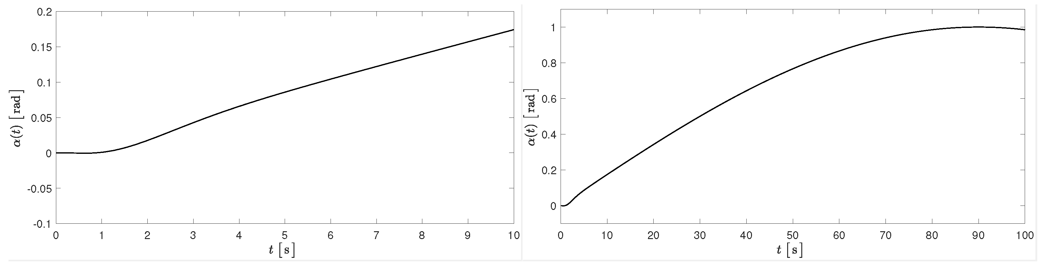
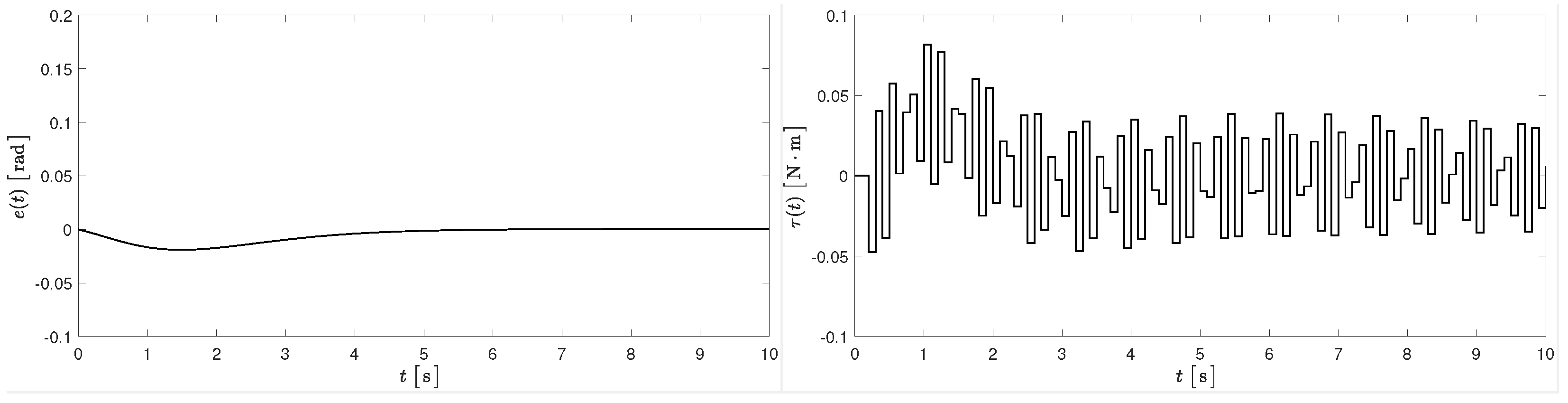
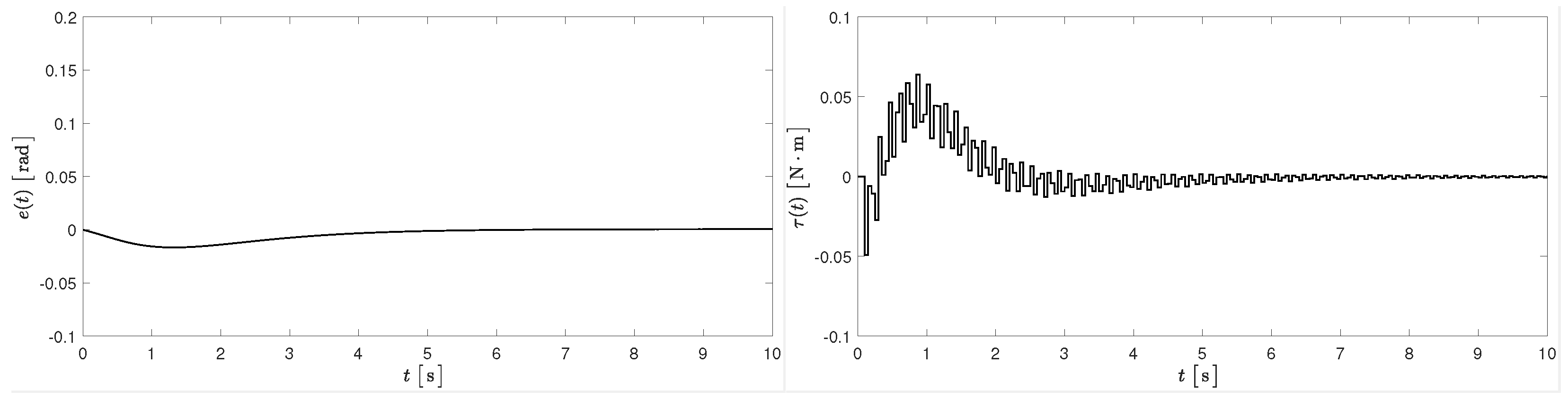
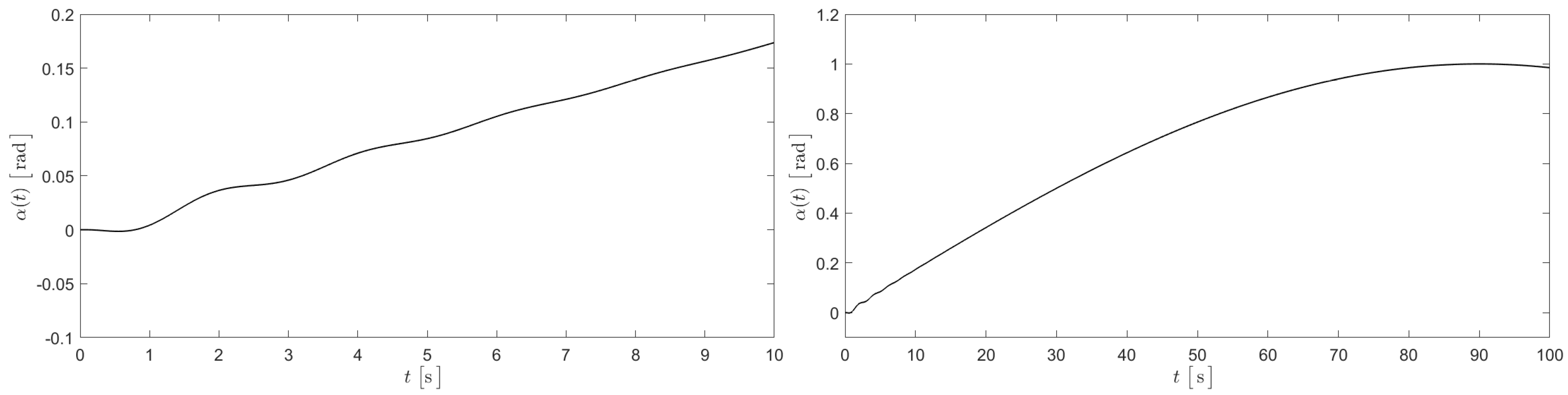
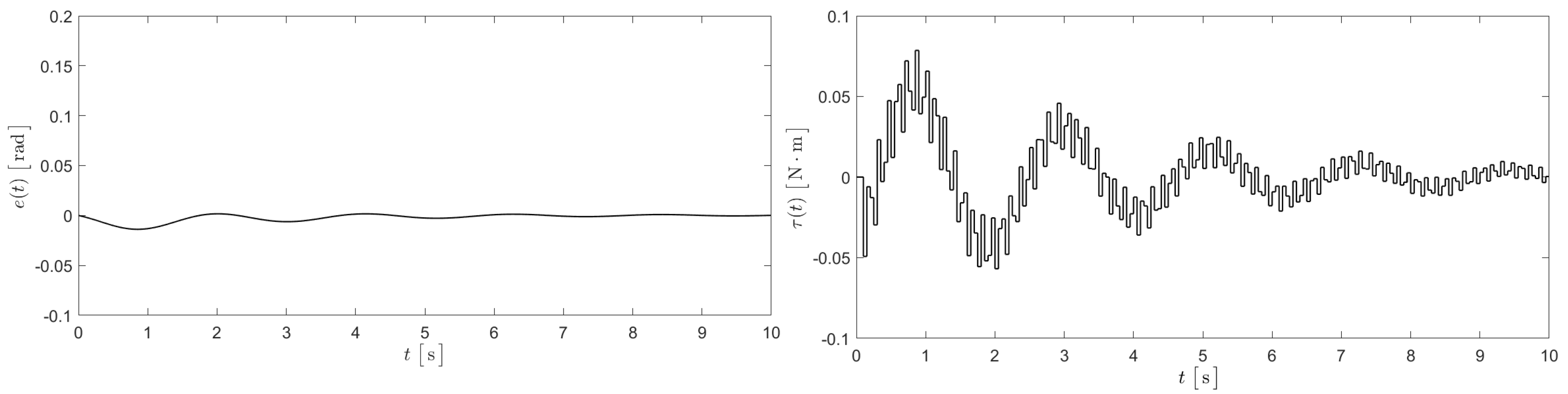
5. Numerical Simulations

In order to verify the applicability of the results, we performed numerical simulations using MATLAB R2024b and its Control System Toolbox [25]. We applied the controller ${\displaystyle {\mathsf{\Sigma }}_K}$ given by (130), designed for the discrete-time unit feedback control system of Figure 2, to the digital control system shown in Figure 3. The data assumed for the computations correspond to the class of microsatellites with weight of 50–100 kg, as detailed in

Table 2. Parameters for the satellite with a solar panel used in the computations.

Parameter	Value
${\displaystyle \hspace{1em}\hspace{1em}\hspace{1em}\hspace{1em}k\left[\frac{\mathrm{N}·\mathrm{m}}{\mathrm{rad}}\right]}$	750
${\displaystyle \hspace{1em}\hspace{1em}\hspace{1em}\hspace{1em}b\left[\mathrm{N}·\mathrm{m}·\mathrm{s}\right]}$	0.01
${\displaystyle \hspace{1em}\hspace{1em}\hspace{1em}\hspace{1em}I\left[\mathrm{kg}·{\mathrm{m}}^2\right]}$	1.7
${\displaystyle \hspace{1em}\hspace{1em}\hspace{1em}\hspace{1em}p\left[\mathrm{kg}·{\mathrm{m}}^2\right]}$	0.1

.

For the reference signal ${\displaystyle {\alpha }_r(t)=asin({\omega }_{r}t)}$, we assume the following:

$$\begin{array}{c}a=1\left[\mathrm{rad}\right],{\omega }_r=1\left[{\displaystyle \frac{deg}{\mathrm{s}}}\right]={\displaystyle \frac{\pi }{180}}\left[{\displaystyle \frac{\mathrm{rad}}{\mathrm{s}}}\right].\hfill \end{array}$$

(132)

For the continuous-time plant ${\displaystyle {\mathsf{\Sigma }}_G}$, we obtain the following state space matrix:

$$\left[\begin{array}{cc}A& B\\ C& 0\end{array}\right]=\left[\begin{array}{ccccc}0& 0& 1& 0& 0\\ 0& 0& 0& 1& 0\\ -441.17& 441.17& -0.0059& 0.0059& 0.5882\\ 7500& -7500& 0.1& -0.1& 0\\ 1& 0& 0& 0& 0\end{array}\right].$$

(133)

The continuous-time exosystem ${\displaystyle {\mathsf{\Sigma }}_S}$ has the following state space matrix:

$$\left[\begin{array}{c}S\\ T\end{array}\right]=\left[\begin{array}{cc}0& 1\\ -0.0003& 0\\ 1& 0\end{array}\right],$$

(134)

with

$$\sigma (S)={\left[\begin{array}{cc}j0.0175& -j0.0175\end{array}\right]}^T,$$

(135)

which generates the continuous-time reference ${\displaystyle {\alpha }_r(t)}$ in the following form:

$${\alpha }_r(t)=sin0.0175t.$$

(136)

The discrete-time step ${\displaystyle h>0}$ is determined according to the sampling frequency of the actual satellite’s attitude angle ${\displaystyle \alpha (t)}$, which depends on its on-board sensors. It is known from the literature that, for small ${\displaystyle h}$ values, the obtained discrete-time models are usually very accurate. In our computations, we assumed the following two values of ${\displaystyle h}$ and the resulting double sampling frequency ${\displaystyle \mu }$:

$$\begin{array}{cccccc}h& =& 0.1\mathrm{s},\hfill & \mu & =& {\displaystyle \frac{2}{h}}=20\mathrm{Hz},\hfill \\ h& =& 0.05\mathrm{s},\hfill & \mu & =& {\displaystyle \frac{2}{h}}=40\mathrm{Hz}.\hfill \end{array}$$

(137)

For these data, we obtain two discrete-time state space matrices:

$$\left[\begin{array}{cc}{A}^d(20)& B^d(20)\\ C^d(20)& D^d(20)\end{array}\right]=\left[\begin{array}{ccccc}0.8942& 0.1058& 0.0947& 0.0053& 0.0088\\ 1.7979& -0.7979& 0.0899& 0.0101& 0.0084\\ -2.1151& 2.1151& 0.8942& 0.1058& 0.1762\\ 35.9570& -35.9570& 1.7983& -0.7983& 0.1673\\ 0.2995& 0.0167& 0.0150& 0.0008& 0.0014\end{array}\right]$$

(138)

and

$$\left[\begin{array}{cc}{A}^d(40)& B^d(40)\\ C^d(40)& D^d(40)\end{array}\right]=\left[\begin{array}{ccccc}0.9076& 0.0924& 0.0477& 0.0023& 0.0031\\ 1.5714& -0.5714& 0.0393& 0.0107& 0.0026\\ -3.6975& 3.6975& 0.9075& 0.0925& 0.1255\\ 62.8574& -62.8574& 1.5723& -0.5723& 0.1034\\ 0.2133& 0.0103& 0.0053& 0.0003& 0.0003.5\end{array}\right],$$

(139)

and two corresponding discrete-time exosystem matrices:

$$\left[\begin{array}{c}{S}^d(20)\\ T^d(20)\end{array}\right]=\left[\begin{array}{cc}1& 0.1\\ 0& 1\\ 0.3162& 0.0158\end{array}\right]$$

(140)

and

$$\left[\begin{array}{c}{S}^d(40)\\ T^d(40)\end{array}\right]=\left[\begin{array}{cc}1& 0.05\\ 0& 1\\ 0.2236& 0.0056\end{array}\right].$$

(141)

In order to solve the regulator Equation (93), we used the lyap procedure from the MATLAB R2024b Control System Toolbox [25] to compute ${\displaystyle \mathsf{\Pi }}$ from (104), after which ${\displaystyle \mathsf{\Gamma }}$ follows from (103). The state feedback gain matrix ${\displaystyle F\in {\mathbb{R}}^{1\times 4}}$ was chosen to minimize the quadratic functional

$$J({\tau }^d)=w_0\sum _{i=0}^{\infty }{(x^d(i))}^T{x}^d(i)+u_0\sum _{i=0}^{\infty }{({\tau }^d(i))}^2,$$

(142)

with weights ${\displaystyle w_0=1}$ and ${\displaystyle u_0=1}$, for the system ${\displaystyle x^d(i+1)=A^d(\mu )x^d(i)+B^d(\mu ){\tau }^d(i)}$ with ${\displaystyle {\tau }^d(i)=-F{x}^d(i)}$. To solve this optimization problem, we used the dlqr procedure from the MATLAB R2024b Control System Toolbox [25]. As a result,

$$F(20)=\left[\begin{array}{cccc}-64.9105& 66.0854& 1.7803& -0.1379\end{array}\right],$$

(143)

with

$$\sigma (A^d(20)-B^d(20)F(20))=\left[\begin{array}{c}-0.8875+j0.4182\\ -0.8875-j0.4182\\ 0.8938\\ 0.8019\end{array}\right],$$

(144)

and

$$F(40)=\left[\begin{array}{cccc}-62.0930& 63.3290& 1.8883& -0.3066\end{array}\right],$$

(145)

with

$$\sigma (A^d(40)-B^d(40)F(40))=\left[\begin{array}{c}-0.6488+j0.7277\\ -0.6488-j0.7277\\ 0.9490\\ 0.8459\end{array}\right].$$

(146)

The output error gain matrix ${\displaystyle \left[\begin{array}{c}{L}_1\\ L_2\end{array}\right]\in {\mathbb{R}}^{6\times 1}}$ was chosen such that ${\displaystyle {\left[\begin{array}{c}{L}_1\\ L_2\end{array}\right]}^T\in {\mathbb{R}}^{1\times 6}}$ minimizes the quadratic cost functional

$$J({\vartheta }^d)=w_1\sum _{i=0}^{\infty }{({\xi }^d(i))}^T{\xi }^d(i)+u_1\sum _{i=0}^{\infty }{({\vartheta }^d(i))}^2,$$

(147)

with weights ${\displaystyle w_1=1}$ and ${\displaystyle u_1=1}$, for the system ${\displaystyle {\xi }^d(i+1)={\left[\begin{array}{cc}{A}^d(\mu )& 0\\ 0& S^d(\mu )\end{array}\right]}^T{\xi }^d(i)+{\left[\begin{array}{cc}{C}^d(\mu )& -T^d(\mu )\end{array}\right]}^T){\vartheta }^d(i)}$ and ${\displaystyle {\vartheta }^d(i)=-{\left[\begin{array}{c}{L}_1\\ L_2\end{array}\right]}^T{\xi }^d(i)}$. Hence,

$$\left[\begin{array}{c}{L}_1(20)\\ L_2(20)\end{array}\right]={\left[\begin{array}{cccccc}40.6359& 40.4759& -4.0984& 82.7493& 39.2876& -0.3458\end{array}\right]}^T,$$

(148)

with

$$\sigma (\left[\begin{array}{cc}{A}^d(20)& 0\\ 0& S^d(20)\end{array}\right]-\left[\begin{array}{c}{L}_1(20)\\ L_2(20)\end{array}\right]\left[\begin{array}{cc}{C}^d(20)& -T^d(20)\end{array}\right])=\left[\begin{array}{c}-0.9016+j0.4265\\ -0.9016-j0.4265\\ 0.6575\\ 0.9021\\ 0.9994+j0.0013\\ 0.9994-j0.0013\end{array}\right],$$

(149)

and

$$\left[\begin{array}{c}{L}_1(40)\\ L_2(40)\end{array}\right]={\left[\begin{array}{cccccc}44.1508& 43.7351& -3.9466& 81.3172& 42.7705& -0.3751\end{array}\right]}^T,$$

(150)

with

$$\sigma (\left[\begin{array}{cc}{A}^d(40)& 0\\ 0& S^d(40)\end{array}\right]-\left[\begin{array}{c}{L}_1(40)\\ L_2(40)\end{array}\right]\left[\begin{array}{cc}{C}^d(40)& -T^d(40)\end{array}\right])=\left[\begin{array}{c}-0.6620+j0.7447\\ -0.6620-j0.7447\\ 0.7390\\ 0.9506\\ 0.9997+j0.0007\\ 0.9997-j0.0007\end{array}\right].$$

(151)

The two obtained versions of the state space matrix for the controller (131), corresponding to ${\displaystyle h=0.1}$ s and ${\displaystyle h=0.05}$ s, are given as follows:

$$\begin{array}{c}\left[\begin{array}{cc}{A}_K(20)& B_K(20)\\ C_K(20)& 0\end{array}\right]\hfill \\ =\left[\begin{array}{ccccccc}\hfill -14.3785& \hfill 2.5844& \hfill -0.4287& \hfill -0.0353& \hfill 12.7940& \hfill 0.5640& \hfill 40.6359\\ \hfill -13.4414& \hfill 1.6982& \hfill -0.4307& \hfill -0.0304& \hfill 12.7432& \hfill 0.5611& \hfill 40.4759\\ \hfill 10.9187& \hfill -9.8364& \hfill 0.6318& \hfill 0.1343& \hfill -1.0824& \hfill 0.2339& \hfill -4.0984\\ \hfill 14.5488& \hfill -40.7775& \hfill 0.4666& \hfill -0.8604& \hfill 26.2287& \hfill 1.3938& \hfill 82.7493\\ \hfill -15.3188& \hfill 2.9592& \hfill -0.4909& \hfill -0.0404& \hfill 13.3595& \hfill 0.6313& \hfill 39.2876\\ \hfill 0.1349& \hfill -0.0261& \hfill 0.0043& \hfill 0.0004& \hfill -0.1088& \hfill 0.9953& \hfill -0.3458\\ \hfill 64.9105& \hfill -66.0854& \hfill -1.7803& \hfill 0.1379& \hfill 1.1748& \hfill 1.6424& \hfill 0\end{array}\right]\hfill \end{array}$$

(152)

and

$$\begin{array}{c}\left[\begin{array}{cc}{A}_K(40)& B_K(40)\\ C_K(40)& 0\end{array}\right]\hfill \\ =\left[\begin{array}{ccccccc}\hfill -9.2751& \hfill 0.4179& \hfill -0.1644& \hfill -0.0129& \hfill 9.8572& \hfill 0.2273& \hfill 44.1508\\ \hfill -8.5477& \hfill -0.2160& \hfill -0.1698& \hfill -0.0045& \hfill 9.7637& \hfill 0.2243& \hfill 43.7351\\ \hfill 5.0198& \hfill -4.2940& \hfill 0.6891& \hfill 0.1324& \hfill -0.7257& \hfill 0.1785& \hfill -3.9466\\ \hfill 50.1649& \hfill -68.4405& \hfill 0.9973& \hfill -0.5703& \hfill 18.2756& \hfill 0.5730& \hfill 81.3172\\ \hfill -10.0530& \hfill 0.5077& \hfill -0.1997& \hfill -0.0157& \hfill 10.5452& \hfill 0.2654& \hfill 42.7705\\ \hfill 0.0882& \hfill -0.0045& \hfill 0.0018& \hfill 0.0001& \hfill -0.0837& \hfill 0.9981& \hfill -0.3751\\ \hfill 62.0930& \hfill -63.3290& \hfill -1.8883& \hfill 0.3066& \hfill 1.2358& \hfill 1.5817& \hfill 0\end{array}\right].\hfill \end{array}$$

(153)

The results of the numerical simulations are shown below, in Figure 4, Figure 5, Figure 6, Figure 7 and Figure 8. Figure 4 shows parts of the exact reference attitude angle ${\displaystyle {\alpha }_r(t)}$, which is sampled in the digital control system shown in Figure 3.

The actual attitude angle ${\displaystyle \alpha (t)}$ of the continuous-time (real) satellite model ${\displaystyle {\mathsf{\Sigma }}_G}$ was computed for the two values of the time step ${\displaystyle h}$, as presented in Figure 5 and Figure 7. Moreover, we also computed the actual continuous-time error ${\displaystyle e(t)}$—defined as the difference between the actual angle ${\displaystyle \alpha (t)}$ and the exact reference angle ${\displaystyle {\alpha }_r(t)}$—in order to show how the discrete-time controller ${\displaystyle {\mathsf{\Sigma }}_K}$ performs in the digital control system of Figure 3. The result is shown in Figure 6 and Figure 8, where the continuous-time control torque ${\displaystyle \tau (t)}$, generated by the ${\displaystyle ZOH}$ and acting on the actual plant ${\displaystyle {\mathsf{\Sigma }}_G}$, is also presented.

It follows from the numerical simulations that, in both considered cases of time step ${\displaystyle h}$, we observed very similar rapid decay of the tracking error ${\displaystyle e(t)}$.

In order to show the robustness of the developed control algorithm, we applied the controller (153)—designed for the plant with parameters from Table 2—in the digital control system for the perturbed plant with the set of parameters ${\displaystyle \overline{k}}$, ${\displaystyle \overline{b}}$, ${\displaystyle \overline{I}}$ and ${\displaystyle \overline{p}}$ given in

Table 3. The perturbed parameters of the satellite with a solar panel.

Parameter	Value
${\displaystyle \hspace{1em}\hspace{1em}\hspace{1em}\hspace{1em}\overline{k}=0.9k\left[\frac{\mathrm{N}·\mathrm{m}}{\mathrm{rad}}\right]}$	675
${\displaystyle \hspace{1em}\hspace{1em}\hspace{1em}\hspace{1em}\overline{b}=1.1b\left[\mathrm{N}·\mathrm{m}·\mathrm{s}\right]}$	0.011
${\displaystyle \hspace{1em}\hspace{1em}\hspace{1em}\hspace{1em}\overline{I}=0.45I\left[\mathrm{kg}·{\mathrm{m}}^2\right]}$	0.765
${\displaystyle \hspace{1em}\hspace{1em}\hspace{1em}\hspace{1em}\overline{p}=1.1p\left[\mathrm{kg}·{\mathrm{m}}^2\right]}$	0.11

.

These parameters led to the following state space matrix of the plant ${\displaystyle {\mathsf{\Sigma }}_{\overline{G}}}$:

$$\left[\begin{array}{cc}\overline{A}& \overline{B}\\ \overline{C}& 0\end{array}\right]=\left[\begin{array}{ccccc}0& 0& 1& 0& 0\\ 0& 0& 0& 1& 0\\ -882.4& 882.4& -0.0144& 0.0144& 1.3072\\ 6136.4& -6136.4& 0.1& -0.1& 0\\ 1& 0& 0& 0& 0\end{array}\right].$$

(154)

The obtained results of the numerical simulations are presented in Figure 9 and Figure 10, which indicate satisfactory and rapid decay of the tracking error ${\displaystyle e(t)}$.

A more elaborate robustness analysis of the developed discrete-time controller (similar to that performed in the study by [20] for the continuous-time case) could be carried out based on the structured singular values; however, this would require further research.

6. Conclusions

The results presented in this paper prove that the combination of the Cayley–Tustin time-discretization scheme and the general regulation theory in the state space setup led to an effective design procedure for a discrete-time controller, which can be directly used in digital satellite attitude control systems with zero-order hold. The advantage of the developed controller is that it only requires the satellite’s sampled attitude angle to be measured, such that no angular velocity measurement is required. The controller matrices involve the feedback gain ${\displaystyle F}$ and the output injection gain ${\displaystyle L}$, which can be computed using LQR algorithms to enable satisfactory behavior of the plant output and tracking error signals. In order to control the behavior of these signals, the scalar weights ${\displaystyle w_0}$, ${\displaystyle u_0}$, and ${\displaystyle w_1}$, ${\displaystyle u_1}$ are used. Instead of the simple scalar weights in Functionals (142) and (147), one can introduce matrices to weigh the state variables selectively and match additional quantitative design objectives such as the overshoot, rise time, and settling time.

The developed procedure is general and easily extendable to more complex multi-variable plants with various time-varying reference signals and disturbances. It follows from the literature (see, e.g., [14]) that the general regulation theory is also successfully applicable in the design of asymptotic tracking controllers for non-linear plants. The author’s plan for future work covers the development of a proper robustness analysis of discrete-time controllers designed for both linear and non-linear plants.

References

1. Narkiewicz, J.; Sochacki, M.; Zakrzewski, B. Generic model of a satellite attitude control system. Int. J. Aerosp. Eng. 2020, 2020, 5352019. [Google Scholar] [CrossRef]
2. Narkiewicz, J.; Grunvald, S.; Sochacki, M. Attitude control system for an earth observation satellite. Bull. Pol. Acad. Sci. Tech. Sci. 2024, 72, e148612. [Google Scholar]
3. Xie, Y.; Huang, H.; Hu, Y.; Zhang, G. Applications of advanced control methods in spacecrafts - progress, challenges, and future prospects. Front. Inf. Technol. Electron. Eng. 2016, 17, 416–428. [Google Scholar] [CrossRef]
4. Wenya, Z.; Haixu, W.; Zhengwei, R.; Zhigang, W.; Enmei, W. High accuracy attitude control system design for satellite with flexible appendages. Math. Probl. Eng. 2014, 695758. [Google Scholar]
5. Wei, H.; Shuzhi, S.G. Dynamic modeling and vibration control of a flexible satellite. IEEE Trans. Aerosp. Electron. Syst. 2015, 51, 1422–1430. [Google Scholar]
6. Wang, J.; Li, D. Experiments study on attitude coupling control method for flexible spacecraft. Acta Astronaut. 2018, 147, 393–402. [Google Scholar] [CrossRef]
7. Angeletti, F.; Gasbarri, P.; Sabatini, M.; Iannelli, P. Design and performance assessment of a distributed vibration suppression system of a large flexible antenna during attitude manoeuvres. Acta Astronaut. 2020, 176, 542–557. [Google Scholar] [CrossRef]
8. Angeletti, F.; Iannelli, P.; Gasbarri, P.; Sabatini, M. End-to-end design of a robust attitude control and vibration suppression system for large space smart structures. Acta Astronaut. 2021, 187, 416–428. [Google Scholar] [CrossRef]
9. Jungteng, M.; Hao, W.; Dongping, J. PDE model-based boundary control of a spacecraft with double flexible appendages under prescribed performance. Adv. Space Res. 2020, 65, 586–597. [Google Scholar]
10. Li, H.; Jia, Q.; Ma, R.; Chen, X. Observer-based robust actuator fault isolation and identification for microsatellite attitude control systems. Aircr. Eng. Aerosp. Technol. 2021, 93, 1145–1155. [Google Scholar] [CrossRef]
11. Govindaraj, T.; Humaloja, J.-P.; Paunenen, L. Robust controllers for a flexible satellite model. Math. Control Relat. Fields 2024, 14, 356–385. [Google Scholar] [CrossRef]
12. El Hariry, M.; Cini, A.; Mellone, G.; Balossino, A. Deep reinforcement learning policies for underactuated satellite attitude control. arXiv 2025, arXiv:2505.00165. [Google Scholar]
13. Francis, B.A. The linear multivariable regulator problem. Siam J. Control Optim. 1977, 15, 486–505. [Google Scholar] [CrossRef]
14. Isidori, A.; Marconi, L.; Serrani, A. Robust Autonomous Guidance An Internal Model Approach; Springer: London, UK, 2003. [Google Scholar]
15. Havu, V.; Malinen, J. The Cayley transform as a time discretization scheme. Integral Equ. Oper. Theory 2007, 28, 825–851. [Google Scholar] [CrossRef]
16. Emirsajłow, Z. Discrete-time output observers for boundary control systems. Int. J. Appl. Math. Comput. Sci. 2021, 31, 613–626. [Google Scholar] [CrossRef]
17. Santana, A.; Martins-Filho, L.; Duarte, R.; Arantes, G.; Casella, I. Attitude control of a satellite by using digital signal processing. J. Aerosp. Technol. Manag. 2012, 4, 15–24. [Google Scholar] [CrossRef]
18. Molina, J.C.; Ayerdi, V.; Zea, L. Attitude control model for CubeSats. In Proceedings of the 2nd IAA Latin American CueSat Workshop, Florianopolis, Brazil, 28 February–2 March 2016; Volume 2. [Google Scholar]
19. Emirsajłow, Z.; Barciński, T.; Bukowiecka, N. Attitude control of an earth observation satellite with a solar panel. In Advanced Contemporary Control; Pawelczyk, M., Bismor, D., Ogonowski, S., Kacprzyk, J., Eds.; Springer Nature: Cham, Switzerland, 2023; pp. 393–402. [Google Scholar]
20. Emirsajłow, Z.; Barciński, T. A robust asymptotic tracking controller for an uncertain 2DOF underactuated mechanical system motivated by a satellite attitude control problem. Int. J. Appl. Math. Comput. Sci. 2025, 35, 97–116. [Google Scholar] [CrossRef]
21. Curtain, R.; Oostveen, J. Bilinear transformations between discrete-time and continuous-time infinite-dimensional systems. In Proceedings of the International Conference on Methods and Models in Automation and Robotics MMAR1997, Międzyzdroje, Poland, 26–30 August 1997; pp. 861–870. [Google Scholar]
22. Ogata, K. Discrete-Time Control Systems; Prentice-Hall: Englewood Cliffs, NJ, USA, 1995. [Google Scholar]
23. Francis, B.A.; Wonham, W.M. The internal model principle for linear multivariable regulators. Appl. Math. Optim. 1975, 2, 170–194. [Google Scholar] [CrossRef]
24. Williams, R.L.; Lawrence, D.A. Linear State-Space Control Systems; John Wiley & Sons: Hoboken, NJ, USA, 2007. [Google Scholar]
25. Matlab Control System Toolbox, Ver. R2024b; MathWorks: Natick, MA, USA, 2024.
Figure 1. Visualization of the observation satellite Sentinel-2 with a solar panel (image: ©ESA/Astrium (left)) and its simplified sketch (right).
Applsci 15 06674 g001
Figure 2. The discrete-time unit feedback control system.
Applsci 15 06674 g002
Figure 3. The digital control system with the continuous-time plant Σ G and Z O H .
Applsci 15 06674 g003
Figure 4. The reference attitude angle α r ( t ) for t [ 0 , 10 ] (left) and t [ 0 , 100 ] (right).
Applsci 15 06674 g004
Figure 5. The actual attitude angle α ( t ) for t [ 0 , 10 ] (left) and t [ 0 , 100 ] (right) for h = 0.1 s.
Applsci 15 06674 g005
Figure 6. The actual error e ( t ) (left) and control torque τ ( t ) (right) for h = 0.1 s .
Applsci 15 06674 g006
Figure 7. The actual attitude angle α ( t ) for t [ 0 , 10 ] (left) and t [ 0 , 100 ] (right) for h = 0.05 s .
Applsci 15 06674 g007
Figure 8. The actual error e ( t ) (left) and the control torque τ ( t ) (right) for h = 0.05 s .
Applsci 15 06674 g008
Figure 9. The actual attitude angle α ( t ) for t [ 0 , 10 ] (left) and t [ 0 , 100 ] (right) for h = 0.05 s .
Applsci 15 06674 g009
Figure 10. The actual error e ( t ) (left) and the control torque τ ( t ) (right) for h = 0.05 s .
Applsci 15 06674 g010