


Classifying X-Ray Tube Malfunctions: AI-Powered CT Predictive Maintenance System


Abstract
1. Introduction
- Corrective maintenance—Existing errors are corrected when they occur;
- Preventive maintenance—Maintenance is performed periodically, on predetermined intervals;
- Predictive maintenance (PdM)—Predicting a malfunction before it happens.
2. Related Work
3. Diagnosing Failures in Medical Equipment
3.1. Structure of the CT Device
- Image Quality Parameters: Resolution and noise levels must be consistently monitored to ensure diagnostic accuracy.
- Dose Parameters: Monitoring radiation exposure to patients is crucial for safety.
- Operational Parameters: Metrics like X-ray tube voltage and current, gantry rotation time, and table movement are critical for system longevity and performance.
3.2. X-Ray Tube Failures
4. Data
4.1. Data Description
- Rotation time—Deviations in the rotation time could indicate a mechanical problem in the gantry rotation system, such as worn bearings or motor malfunction. Such problems might result in excessive vibrations during scanning, which could lead to lower quality of the images or even damage to the X-ray tube and other components.
- Scan duration—Deviation from the expected scanning time may indicate a problem with the patient table or a mechanical issue with the gantry, which can cause reduced image quality and may increase radiation dose. Prolonged scanning times may lead to overheating of components, mechanical wear, and increased radiation exposure, potentially resulting in decreased performance and shorter device lifespan.
- Frequency and current of the cooling pump—could signalise problems with the cooling system in general.
4.2. Data Cleaning
4.2.1. Identifying Anomalies and Handling Them
4.2.2. Excluding Irrelevant Parameters
- Scan Count: Not indicative of the CT device’s condition.
- Date-Time: Assumed constant environmental conditions.
4.3. Data Preparation
4.3.1. Parameter Averaging
4.3.2. Categorical Encoding
4.3.3. Normalisation
4.4. Feature Extraction
4.4.1. Autoregressive Models
4.4.2. Discrete Wavelet Transformation
5. Classifiers
5.1. Classifier Selection
- Logistic Regression (LR);
- Decision Trees (DT);
- Random Forest (RF);
- Gradient Boosting decision trees (GBDT);
- Support Vector Machines (SVM).
- Long short-term memory (LSTM);
- Convolutional Neural Networks (CNN).
5.1.1. Decision Trees, Logistic Regression and SVM
5.1.2. Gradient Boosting Machines and Random Forest
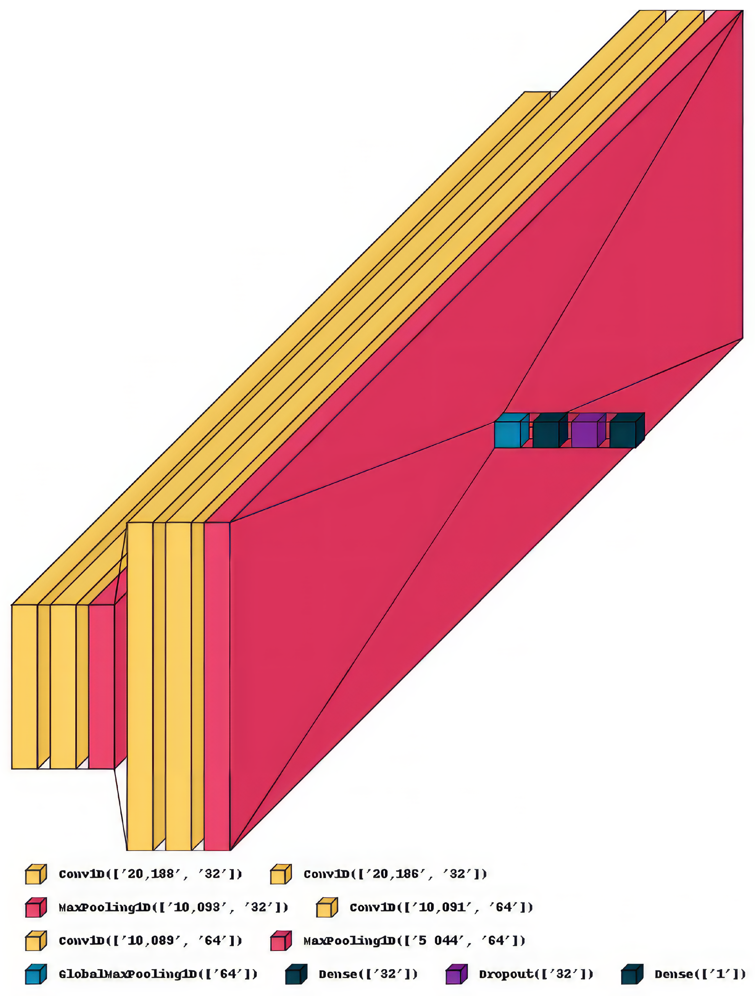
5.1.3. Convolutional Neural Networks
5.1.4. LSTM
- Input gate
- Forget gate
- Output gate
6. Experiments
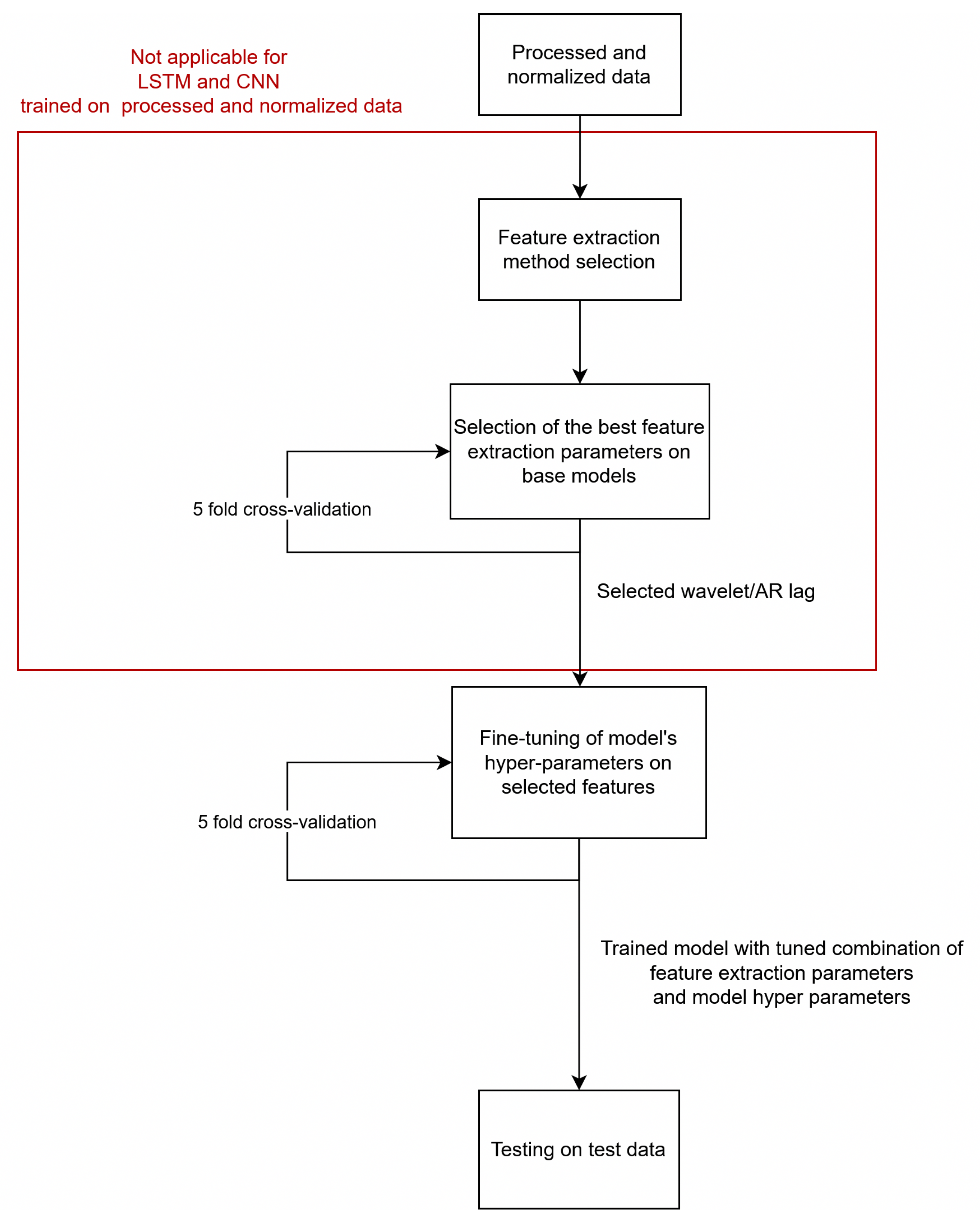
6.1. Methodology
- LR
- –
- penalty—In the range of [l1, l2 and None]
- –
- c—Parameter related to regularisation strength (inverse), in the range of [0.1, 1, 10, 100]
- SVC
- –
- kernels—Selected kernel function, in the range of [“rbf”, “linear”, “poly”]
- –
- c—Same as for LR (1)
- –
- gamma—kernel coefficient, in the range of [0.01, 0.1, 1, 10], base was ’scale’
- RF
- –
- Number of estimators—number of constructed trees, values in [10, 100, 1000, 10,000]
- –
- Distance criterion—possible values were [gini, entropy, log_loss]
- –
- Minimal number of samples in leaf nodes—values were in the range of 1–9 with step 2, base was 1
- DT
- –
- Distance criterion—same as RF
- –
- Minimal number of samples in leaf nodes—same as RF
- GBDT
- –
- Number of estimators—[100, 1000, 10,000]
- –
- Subsamples—Ratio of samples used for training base of learners—[0.75, 1], base 1
- –
- Maximum depth for base learners—[5, 7, 9], base 6
- –
- Learning rate—[0.1, 0.2], base 0.3
6.2. Autoregressive Model Coefficients as Features
- As mentioned in Section 4.4.1, we treated lag as an hyperparameter. We selected lags spanning from 0 to 10 for testing
- For every lag, every classifier with default parameters was trained
- Afterwards, we selected the best lag for every model based on the accuracy score on the validation set
- We tried to optimise the classifier-specific hyperparameters (listed in Section 6.1) to maximise the validation accuracy
- Finally, we tested the best candidate for every classifier
6.3. DWT Coefficients as Features
- We treated the wavelet shape as a hyperparameter. We selected and tried haar, db1-db10, sym2-sym10, coif1-10
- For every wavelet, every classifier with default parameters was trained
- Afterwards, we selected the best wavelet for every model based on the accuracy score on the validation set
- We tried to optimise the classifier-specific hyperparameters (listed in Section 6.1) to maximise the validation accuracy
- Finally, we tested the best candidate for every classifier
6.4. Experiments with CNN
- 8, 16
- 16, 32
- 32, 64
- 64, 128
- 8, 16, 32
- 16, 32, 64
- 32, 64, 128
- 64, 128, 256
6.5. RNN-Based Processing
7. Summary
- The model likely can spot all the malfunctioning X-ray tubes.
- If the model classifies an X-ray tube as working, it has only a small chance (never before seen malfunctions) of the tube being replaced too soon.
- Gather more data—Data quantity is essential for good performance and generalisation, which is even more so for deep learning-based models.
- Create a fully retrospective study—All the X-ray tubes classified as working during the study were still working by the time of log gathering. That means there was no way to obtain more information about their expected life cycle. While, for the purpose of classification as being malfunctioning or still working, this was not a problem, it became a problem when intervals from the start of the life cycle were selected. For future work, this would allow us to obtain more information on the life cycle.
- Inspect failed X-ray tubes—In order to allow for more granular classification, a detailed understanding of the cause of failure would be needed.
- Conduct a deeper analysis of the features and their impact on the model—as different features can contribute to various types of faults at different stages of the life cycle. There is room for further experimentation with different features. Afterwards, explainable AI methods such as SHAP [57], or its extension to recurrent models—TimeSHAP [58], could be utilised.
Author Contributions
Funding
Institutional Review Board Statement
Informed Consent Statement
Data Availability Statement
Conflicts of Interest
Appendix A

| Parameter Name | Description |
|---|---|
| scan_count | Number of scans since installation of tube. |
| date_time | Scan date and time (up to seconds). |
| rot_time | 10 ms Time of rotation for this scan. |
| voltage | 1/100 V Tube voltage during scan, represented by two parameters: nominal and actual voltage. |
| scan_time | 1/10 ms Scan duration (with X-ray), represent by two parameters: nominal and actual scan time. |
| stator_frequency | Hz Stator magnetic field rotation speed. |
| anode_frequency | Hz Anode rotation speed. |
| kind | Type of scanning: STA—the table does not move, SPI—the X-ray tube rotates while the table with the patient moves, a spiral is created, SEQ—sequence of scans, ROT—the X-ray tube rotates while the table does not move, it moves only after completing the rotation, ZIG—the table moves back and forth during the entire scan for a specific purpose, TOP—an image is created from one angle, the table moves, like a regular X-ray image. |
| flying_focal_spot | Position of the focal spot (the area of the anode surface which receives the beam of electrons from the cathode) of the X-ray tube: DIAG—flying focal spot is positioned diagonally relative to the gantry, PHI—flying focal spot is positioned along a fixed angle relative to the gantry, PHIs—is similar to the Phi mode, but the angle of the flying focal spot can be adjusted, NONE—fixed focal spot is used. |
| current | mA Current supplied to the tube, represented by seven parameters: current that is displayed to the user on the interface (ui), nominal, minimum, maximum, mean during scan, at scan begin, at scan end. |
| focus | The size of the X-ray beam at the point where it is emitted from the X-ray tube: SHR—super high resolution, SUHR—super ultra-high resolution, FHR—fine high resolution, UHR—ultra-high resolution, GET—geometry enhanced tool, LO—low output, SP—super position. |
| filament_current | mA Current supplied to the filament, represent by three parameters: filament current nominal, at scan begin, at scan end. |
| dose | mV Amount of radiation released, represent by four parameters: dose nominal, minimum, maximum, at scan end. |
| water_inlet_temp | 1 °C water temperature at tube inlet, represent by two parameters: temperature for scan begin and after scan end. |
| water_outlet_temp | 1 °C water temperature at tube outlet, represent by two parameters: temperature for scan begin and after scan end. |
| oil_temp | 1 °C Temperature of the tube system, represent by two parameters: temperature for scan begin and after scan end. |
| cooling_liquid_temp | 1 °C The calculated anode temperature at the scan end. |
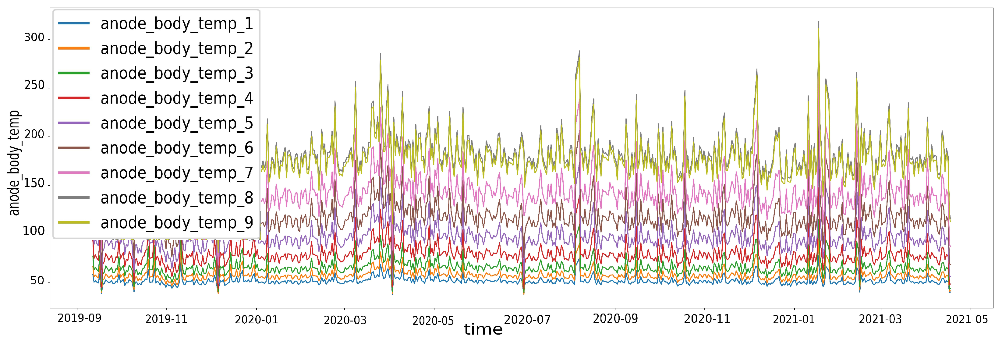
| anode_body_temp | 1 °C Calculated anode surface temperature at scan end, represent by nine parameters, where each parameter is a point on the anode. |
| focal_track_temp | 1 °C Calculated focal track temperature at scan end, represent by nine parameters, where each parameter is a point on focal track. |
| temp_focal_spot | 1 °C Temperature of focal spot of the X-ray tube. |
| e_catcher_temp | 1 °C Calculated E-catcher temperature at scan end. |
| tank_expansion | mm Indicates the status of the expansion cooling tank with an distance sensor. |
| gantry_temp | 1 °C Gantry temperature at scan end. |
| cooling_pump_frequency | Hz Cooling pump rotation speed. |
| cooling_pump_current | mA Cooling pump current. |
| hv_block_temp | 1 °C High Voltage block temperature. |
| stator_current | mA Current of the stator. |
| arcs | Number of tube arcings during scan. |
| arcs_half_ut | Number of tube half arcings during scan. |
| xc_drops | Sum over the whole scan of signal stop inverter. |
| hv_drops | Sum of High Voltage drops over the whole scan. |
| start_angle | Angle for first valid reading. |
| readings | Total sum of all readings over the scan. |
| defective_readings | Total sum of all defect readings over the scan. |
| last_defective_reading | Last defect reading. |
| mode | Scan Mode (A,B)—using of 1 or 2 X-rays. |
| abort_reason | Reason why a CT scan was aborted: SuspendedByUser—scan was intentionally paused or suspended by the user, StoppedByUser—the scan was stopped by the user before completion, Comp—scan was interrupted due to a problem with the CT system’s computer, Abort— interruption of the scan for some reason other than the above. |
| abort_controller | Specific type of abort controller that stops the scan. |
| DOM_type | Type of digital output module used in the control system. |
| eco | State refers to the eco mode setting of the machine (off, on). |
Appendix B
| Parameter Name | Value |
|---|---|
| scan_count | 301,196 |
| kind | SEQ |
| date_time | 8 January 2023 18:56:36 |
| rot_time | 1.0 |
| scan_time_nom | 2.0 |
| scan_time_act | 2.0 |
| voltage_nom | 120 |
| voltage_act | 119.9 |
| current_ui | 165 |
| current_nom | 156 |
| current_min | 130 |
| current_max | 133 |
| current_control | 133 |
| current_mean | 133 |
| current_begin | 147 |
| current_end | 133 |
| focus | LO |
| stator_frequency | 220 |
| anode_frequency | 199 |
| filament_current_nom | 1621 |
| filament_current_begin | 1604 |
| filament_current_control | 1605 |
| filament_current_end | 1605 |
| filament_push_current | 1627 |
| dose_nom | 4131 |
| dose_min | 2576 |
| dose_max | 3874 |
| dose_end | 3476 |
| flying_focal_spot | Phi |
| water_inlet_temp_begin | 41 |
| water_inlet_temp_end | 41 |
| water_outlet_temp_begin | 41 |
| water_outlet_temp_end | 41 |
| oil_temp_1_begin | 42 |
| oil_temp_1_end | 42 |
| oil_temp_2_begin | 43 |
| oil_temp_2_end | 44 |
| e_catcher_temp | 43 |
| cooling_liquid_temp | 32 |
| temp_focal_spot | 214 |
| gantry_temp | 28 |
| cooling_pump_frequency | 83 |
| cooling_pump_current | 6277 |
| hv_block_temp | 40 |
| stator_current | 12,891 |
| xc_drops | 1 |
| hv_drops | 0 |
| start_angle | 48,928 |
| readings | 5600 |
| defective_readings | 0 |
| last_defective_reading | 0 |
| DOM_type | ZEC |
| mode | A |
| abort_reason | Comp |
| abort_controller | NaN |
| focal_track_temp | 193.0 |
| anode_body_temp | 71.666667 |
Appendix C
| Predicted Working | Predicted Replaced | |
|---|---|---|
| Actual working | 10 | 4 |
| Actual replaced | 0 | 12 |
| Predicted Working | Predicted Replaced | |
|---|---|---|
| Actual working | 12 | 2 |
| Actual replaced | 0 | 12 |
| Predicted Working | Predicted Replaced | |
|---|---|---|
| Actual working | 9 | 5 |
| Actual replaced | 0 | 12 |
| Predicted Working | Predicted Replaced | |
|---|---|---|
| Actual working | 10 | 4 |
| Actual replaced | 0 | 12 |
| Predicted Working | Predicted Replaced | |
|---|---|---|
| Actual working | 12 | 2 |
| Actual replaced | 0 | 12 |
References
- UNSCEAR. Sources, Effects and Risks of Ionizing Radiation, United Nations Scientific Committee on the Effects of Atomic Radiation (UNSCEAR) 2020/2021 Report, Volume IV: Scientific Annex D-Evaluation of Occupational Exposure to Ionizing Radiation; United Nations: New York, NY, USA, 2022. [Google Scholar]
- Achouch, M.; Dimitrova, M.; Ziane, K.; Sattarpanah Karganroudi, S.; Dhouib, R.; Ibrahim, H.; Adda, M. On predictive maintenance in industry 4.0: Overview, models, and challenges. Appl. Sci. 2022, 12, 8081. [Google Scholar] [CrossRef]
- Manchadi, O.; Ben-Bouazza, F.E.; Jioudi, B. Predictive maintenance in healthcare system: A survey. IEEE Access 2023, 11, 61313–61330. [Google Scholar] [CrossRef]
- Nunes, P.; Santos, J.; Rocha, E. Challenges in predictive maintenance–A review. CIRP J. Manuf. Sci. Technol. 2023, 40, 53–67. [Google Scholar] [CrossRef]
- Saufi, S.R.; Ahmad, Z.A.B.; Leong, M.S.; Lim, M.H. Challenges and opportunities of deep learning models for machinery fault detection and diagnosis: A review. IEEE Access 2019, 7, 122644–122662. [Google Scholar] [CrossRef]
- Cen, J.; Yang, Z.; Liu, X.; Xiong, J.; Chen, H. A review of data-driven machinery fault diagnosis using machine learning algorithms. J. Vib. Eng. Technol. 2022, 10, 2481–2507. [Google Scholar] [CrossRef]
- Wahed, M.A.; Sharawi, A.A.; Badawi, H.A. Modeling of medical equipment maintenance in health care facilities to support decision making. In Proceedings of the 2010 5th Cairo International Biomedical Engineering Conference, Cairo, Egypt, 16–18 December 2010; IEEE: Piscataway, NJ, USA, 2010; pp. 202–205. [Google Scholar]
- Packianather, M.S.; Munizaga, N.L.; Zouwail, S.; Saunders, M. Development of soft computing tools and IoT for improving the performance assessment of analysers in a clinical laboratory. In Proceedings of the 2019 14th Annual Conference System of Systems Engineering (SoSE), Cairo, Egypt, 16–18 December 2010; IEEE: Piscataway, NJ, USA, 2019; pp. 158–163. [Google Scholar]
- Kovačević, Ž.; Gurbeta Pokvić, L.; Spahić, L.; Badnjević, A. Prediction of medical device performance using machine learning techniques: Infant incubator case study. Health Technol. 2020, 10, 151–155. [Google Scholar] [CrossRef]
- Badnjević, A.; Pokvić, L.G.; Hasičić, M.; Bandić, L.; Mašetić, Z.; Kovačević, Ž.; Kevrić, J.; Pecchia, L. Evidence-based clinical engineering: Machine learning algorithms for prediction of defibrillator performance. Biomed. Signal Process. Control 2019, 54, 101629. [Google Scholar] [CrossRef]
- Gonzalez-Dominguez, J.; Sánchez-Barroso, G.; Aunion-Villa, J.; Garcia-Sanz-Calcedo, J. Markov model of computed tomography equipment. Eng. Fail. Anal. 2021, 127, 105506. [Google Scholar] [CrossRef]
- Cardona Ortegón, A.F.; Guerrero, W.J. Optimizing maintenance policies of computed tomography scanners with stochastic failures. In Service Oriented, Holonic and Multi-Agent Manufacturing Systems for Industry of the Future: Proceedings of SOHOMA LATIN AMERICA 2021, Bogota, Colombia, 27–28 January 2021; Springer: Berlin/Heidelberg, Germany, 2021; pp. 331–342. [Google Scholar]
- Mohd, M.H.S.E.B.; Shazril, A.; Mashohor, S.; Amran, M.E.; Hafiz, N.F.; Rahman, A.A.; Ali, A.; Rasid, M.F.A.; Kamil, A.S.A.; Azilah, N.F. Predictive Maintenance Method using Machine Learning for IoT Connected Computed Tomography Scan Machine. In Proceedings of the 2023 IEEE 2nd National Biomedical Engineering Conference (NBEC), Melaka, Malaysia, 5–7 September 2023; IEEE: Piscataway, NJ, USA, 2023; pp. 42–47. [Google Scholar]
- Azrul, M.H.S.E.M.; Mashohor, S.; Amran, M.E.; Hafiz, N.F.; Ali, A.M.; Naseri, M.S.; Rasid, M.F.A. Assessment of IoT-Driven Predictive Maintenance Strategies for Computed Tomography Equipment: A Machine Learning Approach. IEEE Access 2024. [Google Scholar]
- Zhou, H.; Liu, Q.; Liu, H.; Chen, Z.; Li, Z.; Zhuo, Y.; Li, K.; Wang, C.; Huang, J. Healthcare facilities management: A novel data-driven model for predictive maintenance of computed tomography equipment. Artif. Intell. Med. 2024, 149, 102807. [Google Scholar] [CrossRef]
- Zhong, J.; Zhang, H.; Liu, Q.; Miao, Q.; Huang, J. Prognosis for Filament Degradation of X-Ray Tubes Based on IoMT Time Series Data. IEEE Internet Things J. 2024, 12, 8084–8094. [Google Scholar] [CrossRef]
- Amoore, J.N. A structured approach for investigating the causes of medical device adverse events. J. Med Eng. 2014, 2014, 314138. [Google Scholar] [CrossRef] [PubMed]
- Ward, J.R.; Clarkson, P.J. An analysis of medical device-related errors: Prevalence and possible solutions. J. Med Eng. Technol. 2004, 28, 2–21. [Google Scholar] [CrossRef] [PubMed]
- Laganà, F.; Bibbɂ, L.; Calcagno, S.; De Carlo, D.; Pullano, S.A.; Pratticɂ, D.; Angiulli, G. Smart Electronic Device-Based Monitoring of SAR and Temperature Variations in Indoor Human Tissue Interaction. Appl. Sci. 2025, 15, 2439. [Google Scholar] [CrossRef]
- Kemerink, M.; Dierichs, T.J.; Dierichs, J.; Huynen, H.; Wildberger, J.E.; van Engelshoven, J.M.; Kemerink, G.J. The application of X-rays in radiology: From difficult and dangerous to simple and safe. Am. J. Roentgenol. 2012, 198, 754–759. [Google Scholar] [CrossRef]
- Anburajan, M.; Sharma, J.K. Overview of X-Ray Tube Technology. Biomedical Engineering and its Applications in Healthcare; Springer: Singapore, 2019; pp. 519–547. [Google Scholar]
- The Royal College of Radiologists; Society and College of Radiographers; Institute of Physics and Engineering in Medicine. CT Equipment, Operations, Capacity and Planning in the NHS; Technical report; Institute of Physics and Engineering in Medicine: London, UK, 2015. [Google Scholar]
- England, N.; Improvement, N. Transforming imaging services in England: A national strategy for imaging networks. NHS Improv. Publ. Code CG 2019, 51, 19. [Google Scholar]
- Canadian Agency for Drugs and Technologies in Health. Canadian Medical Imaging Inventory 2022–2023: CT: CMII Report; Canadian Agency for Drugs and Technologies in Health: Ottawa, ON, USA, 2024.
- Parzen, E. Some recent advances in time series modeling. IEEE Trans. Autom. Control 1974, 19, 723–730. [Google Scholar] [CrossRef]
- Kotu, V.; Deshpande, B. Data Science: Concepts and Practice; Morgan Kaufmann: Cambridge, MA, USA, 2018. [Google Scholar]
- Kurzynski, M.; Krysmann, M.; Trajdos, P.; Wolczowski, A. Multiclassifier system with hybrid learning applied to the control of bioprosthetic hand. Comput. Biol. Med. 2016, 69, 286–297. [Google Scholar] [CrossRef]
- Poularikas, A.D. The Transforms and Applications Handbook; Technical report; CRC Press: Boca Raton, FL, USA, 2000. [Google Scholar]
- Burrus, C.S.; Gopinath, R.A.; Guo, H. Wavelets and wavelet transforms. Rice Univ. Houst. Ed. 1998, 98, 7–8. [Google Scholar]
- Bonnevay, S.; Cugliari, J.; Granger, V. Predictive maintenance from event logs using wavelet-based features: An industrial application. In Proceedings of the 14th International Conference on Soft Computing Models in Industrial and Environmental Applications (SOCO 2019), Seville, Spain, 13–15 May 2019; Proceedings 14. Springer: Cham, Switzerland, 2020; pp. 132–141. [Google Scholar]
- Bhavsar, K.; Vakharia, V.; Chaudhari, R.; Vora, J.; Pimenov, D.Y.; Giasin, K. A Comparative Study to Predict Bearing Degradation Using Discrete Wavelet Transform (DWT), Tabular Generative Adversarial Networks (TGAN) and Machine Learning Models. Machines 2022, 10, 176. [Google Scholar] [CrossRef]
- Zhang, C.; Liu, C.; Zhang, X.; Almpanidis, G. An up-to-date comparison of state-of-the-art classification algorithms. Expert Syst. Appl. 2017, 82, 128–150. [Google Scholar] [CrossRef]
- De Ville, B. Decision trees. Wiley Interdiscip. Rev. Comput. Stat. 2013, 5, 448–455. [Google Scholar] [CrossRef]
- Kleinbaum, D.G.; Dietz, K.; Gail, M.; Klein, M.; Klein, M. Logistic Regression; Springer: Berlin/Heidelberg, Germany, 2002. [Google Scholar]
- Boser, B.E.; Guyon, I.M.; Vapnik, V.N. A training algorithm for optimal margin classifiers. In Proceedings of the Fifth Annual Workshop on Computational Learning Theory, New York, NY, USA, 27–29 July 1992; COLT ’92. pp. 144–152. [Google Scholar] [CrossRef]
- Friedman, J.H. Greedy function approximation: A gradient boosting machine. Ann. Stat. 2001, 29, 1189–1232. [Google Scholar] [CrossRef]
- Breiman, L. Random forests. Mach. Learn. 2001, 45, 5–32. [Google Scholar] [CrossRef]
- Sutton, C.D. Classification and regression trees, bagging, and boosting. Handb. Stat. 2005, 24, 303–329. [Google Scholar]
- Shang, L.; Zhang, Z.; Tang, F.; Cao, Q.; Pan, H.; Lin, Z. CNN-LSTM hybrid model to promote signal processing of ultrasonic guided lamb waves for damage detection in metallic pipelines. Sensors 2023, 23, 7059. [Google Scholar] [CrossRef] [PubMed]
- Kiranyaz, S.; Ince, T.; Abdeljaber, O.; Avci, O.; Gabbouj, M. 1-D convolutional neural networks for signal processing applications. In Proceedings of the ICASSP 2019–2019 IEEE International Conference on Acoustics, Speech and Signal Processing (ICASSP), Brighton, UK, 12–17 May 2019; IEEE: Piscataway, NJ, USA, 2019; pp. 8360–8364. [Google Scholar]
- Chen, L.; Li, S.; Bai, Q.; Yang, J.; Jiang, S.; Miao, Y. Review of image classification algorithms based on convolutional neural networks. Remote Sens. 2021, 13, 4712. [Google Scholar] [CrossRef]
- Alzubaidi, L.; Zhang, J.; Humaidi, A.J.; Al-Dujaili, A.; Duan, Y.; Al-Shamma, O.; Santamaría, J.; Fadhel, M.A.; Al-Amidie, M.; Farhan, L. Review of deep learning: Concepts, CNN architectures, challenges, applications, future directions. J. Big Data 2021, 8, 53. [Google Scholar] [CrossRef]
- Sharma, V.; Gupta, M.; Kumar, A.; Mishra, D. Video processing using deep learning techniques: A systematic literature review. IEEE Access 2021, 9, 139489–139507. [Google Scholar] [CrossRef]
- Simonyan, K.; Zisserman, A. Very Deep Convolutional Networks for Large-Scale Image Recognition. arXiv 2015, arXiv:1409.1556. [Google Scholar] [CrossRef]
- Schmidt, R.M. Recurrent neural networks (rnns): A gentle introduction and overview. arXiv 2019, arXiv:1912.05911. [Google Scholar]
- Mienye, I.D.; Swart, T.G.; Obaido, G. Recurrent neural networks: A comprehensive review of architectures, variants, and applications. Information 2024, 15, 517. [Google Scholar] [CrossRef]
- Hochreiter, S. Untersuchungen zu dynamischen neuronalen Netzen. Diploma, Tech. Univ. München 1991, 91, 31. [Google Scholar]
- Keras. 2015. Available online: https://keras.io (accessed on 10 April 2025).
- Abadi, M.; Agarwal, A.; Barham, P.; Brevdo, E.; Chen, Z.; Citro, C.; Corrado, G.S.; Davis, A.; Dean, J.; Devin, M.; et al. TensorFlow: Large-Scale Machine Learning on Heterogeneous Systems. 2015. Available online: https://www.tensorflow.org/ (accessed on 10 April 2025).
- Buitinck, L.; Louppe, G.; Blondel, M.; Pedregosa, F.; Mueller, A.; Grisel, O.; Niculae, V.; Prettenhofer, P.; Gramfort, A.; Grobler, J.; et al. API design for machine learning software: Experiences from the scikit-learn project. arXiv 2013, arXiv:1309.0238. [Google Scholar] [CrossRef]
- Chen, T.; Guestrin, C. XGBoost: A Scalable Tree Boosting System. In Proceedings of the Proceedings of the 22nd ACM SIGKDD International Conference on Knowledge Discovery and Data Mining, New York, NY, USA, 13–17 August 2016; KDD ’16. pp. 785–794. [Google Scholar] [CrossRef]
- Seabold, S.; Perktold, J. statsmodels: Econometric and statistical modeling with python. In Proceedings of the 9th Python in Science Conference, Austin, TX, USA, 28–30 June 2010. [Google Scholar]
- Lee, G.; Gommers, R.; Waselewski, F.; Wohlfahrt, K.; O’Leary, A. PyWavelets: A Python package for wavelet analysis. J. Open Source Softw. 2019, 4, 1237. [Google Scholar] [CrossRef]
- Gavrikov, P. Visualkeras. 2020. Available online: https://github.com/paulgavrikov/visualkeras (accessed on 10 April 2025).
- Dickey, D.; Fuller, W. Distribution of the Estimators for Autoregressive Time Series With a Unit Root. JASA J. Am. Stat. Assoc. 1979, 74, 427–431. [Google Scholar] [CrossRef]
- Lin, W.; Hasenstab, K.; Moura Cunha, G.; Schwartzman, A. Comparison of handcrafted features and convolutional neural networks for liver MR image adequacy assessment. Sci. Rep. 2020, 10, 20336. [Google Scholar] [CrossRef] [PubMed]
- Lundberg, S.M.; Lee, S.I. A Unified Approach to Interpreting Model Predictions. In Advances in Neural Information Processing Systems 30; Guyon, I., Luxburg, U.V., Bengio, S., Wallach, H., Fergus, R., Vishwanathan, S., Garnett, R., Eds.; Curran Associates, Inc.: Red Hook, NY, USA, 2017; pp. 4765–4774. [Google Scholar]
- Bento, J.; Saleiro, P.; Cruz, A.F.; Figueiredo, M.A.; Bizarro, P. Timeshap: Explaining recurrent models through sequence perturbations. In Proceedings of the 27th ACM SIGKDD conference on Knowledge Discovery & Data Mining, Virtual, 14–18 August 2021; pp. 2565–2573. [Google Scholar]
- He, K.; Zhang, X.; Ren, S.; Sun, J. Deep Residual Learning for Image Recognition. arXiv 2015, arXiv:1512.03385. [Google Scholar] [CrossRef]
- Ahmed, S.; Nielsen, I.E.; Tripathi, A.; Siddiqui, S.; Ramachandran, R.P.; Rasool, G. Transformers in time-series analysis: A tutorial. Circuits Syst. Signal Process. 2023, 42, 7433–7466. [Google Scholar] [CrossRef]
- Zeng, A.; Chen, M.; Zhang, L.; Xu, Q. Are transformers effective for time series forecasting? In Proceedings of the AAAI Conference on Artificial Intelligence, Washington, DC, USA, 7–14 February 2023. [Google Scholar]


| Model | Parameters | AR Lag | Accuracy/Micro F1-Score |
|---|---|---|---|
| LR | c = 1, penalty = L2 | 7 | 72.2% |
| SVC | c = 100, gamma = 0.1, rbf kernel | 6 | 71.6% |
| RF | Estimators = 10,000 criterion = “logloss”/“entropy” Minimal number of samples for leaf = 1 | 3 | 83.4% |
| DT | criterion = “logloss”/“entropy” Minimal number of samples for leaf = 5 | 1 | 75.4% |
| GBDT | Estimators = 100 Subsample = 0.75 Depth = 5/7/9, Learning rate = 0.2 | 6 | 76.2% |
| Model | Parameters | Wavelet | Accuracy/Micro F1-Score |
|---|---|---|---|
| LR | c = 1, penalty = L1 | coif10 | 84% |
| SVC | 16 different setups | coif10 | 84% |
| RF | Estimators = 100 criterion = “gini”, Minimal number of samples for leaf = 9 | coif3 | 68.4% |
| DT | criterion = “gini”, Minimal number of samples for leaf = 7 | db5 | 65.4% |
| GBDT | Estimators = 1000, Subsample = 0.75 Depth = 5/7/9, Learning rate = 0.2 | coif2 | 70.6% |
| Model | Features | Parameters | Accuracy |
|---|---|---|---|
| LSTM | DWT | Haar | 61.8% |
| normalised samples | 32 units | 87% | |
| VGG-like | DWT | coif7 | 78.6% |
| normalised samples | 32, 64 filters | 75.4% |
Disclaimer/Publisher’s Note: The statements, opinions and data contained in all publications are solely those of the individual author(s) and contributor(s) and not of MDPI and/or the editor(s). MDPI and/or the editor(s) disclaim responsibility for any injury to people or property resulting from any ideas, methods, instructions or products referred to in the content. |
© 2025 by the authors. Licensee MDPI, Basel, Switzerland. This article is an open access article distributed under the terms and conditions of the Creative Commons Attribution (CC BY) license (https://creativecommons.org/licenses/by/4.0/).
Share and Cite
Pomšár, L.; Tsvietaieva, M.; Krupáš, M.; Zolotová, I. Classifying X-Ray Tube Malfunctions: AI-Powered CT Predictive Maintenance System. Appl. Sci. 2025, 15, 6547. https://doi.org/10.3390/app15126547
Pomšár L, Tsvietaieva M, Krupáš M, Zolotová I. Classifying X-Ray Tube Malfunctions: AI-Powered CT Predictive Maintenance System. Applied Sciences. 2025; 15(12):6547. https://doi.org/10.3390/app15126547
Chicago/Turabian StylePomšár, Ladislav, Maryna Tsvietaieva, Maros Krupáš, and Iveta Zolotová. 2025. "Classifying X-Ray Tube Malfunctions: AI-Powered CT Predictive Maintenance System" Applied Sciences 15, no. 12: 6547. https://doi.org/10.3390/app15126547
APA StylePomšár, L., Tsvietaieva, M., Krupáš, M., & Zolotová, I. (2025). Classifying X-Ray Tube Malfunctions: AI-Powered CT Predictive Maintenance System. Applied Sciences, 15(12), 6547. https://doi.org/10.3390/app15126547