Image-Based Malicious Network Traffic Detection Framework: Data-Centric Approach

Abstract

With the advancement of network communication technology and Internet of Everything (IoE) technology, which connects all edge devices to the internet, the network traffic generated in various platform environments is rapidly increasing. The increase in network traffic makes it more difficult for the detection system to analyze and detect malicious network traffic generated by malware or intruders. Additionally, processing high-dimensional network traffic data requires substantial computational resources, limiting real-time detection capabilities in practical deployments. Artificial intelligence (AI) algorithms have been widely used to detect malicious traffic, but most previous work focused on improving accuracy with various AI algorithms. Many existing methods, in pursuit of high accuracy, directly utilize the extensive raw features inherent in network traffic. This often leads to increased computational overhead and heightened complexity in detection models, potentially degrading overall system performance and efficiency. Furthermore, high-dimensional data often suffers from the curse of dimensionality, where the sparsity of data in high-dimensional space leads to overfitting, poor generalization, and increased computational complexity. This paper focused on feature engineering instead of AI algorithm selections, presenting an approach that uniquely balances detection accuracy with computational efficiency through strategic dimensionality reduction. For feature engineering, two jobs were performed: feature representations and feature analysis and selection. With effective feature engineering, we can reduce system resource consumption in the training period while maintaining high detection accuracy. We implemented a malicious network traffic detection framework based on Convolutional Neural Network (CNN) with our feature engineering techniques. Unlike previous approaches that use one-hot encoding, which increases dimensionality, our method employs label encoding and information gain to preserve critical information while reducing feature dimensions. The performance of the implemented framework was evaluated using the NSL-KDD dataset, which is the most widely used for intrusion detection system (IDS) performance evaluation. As a result of the evaluation, our framework maintained high classification accuracy while improving model training speed by approximately 17.47% and testing speed by approximately 19.44%. This demonstrates our approach’s ability to achieve a balanced performance, enhancing computational efficiency without sacrificing detection accuracy—a critical challenge in intrusion detection systems. With the reduced features, we achieved classification results of a precision of 0.9875, a recall of 0.9930, an F1-score of 0.9902, and an accuracy of 99.06%, with a false positive rate of 0.65%.

1. Introduction

With the development of wired and wireless network communication technology and the increased use of smart devices, such as smartphones and tablets, internet accessibility has increased, leading to an exponential increase in network traffic volume. Moreover, with the emergence of cutting-edge IoE (Internet of Everything)-based technologies like Cloud Computing, Smart Grid, and Vehicle-to-Everything (V2X), the volume of network traffic has surged in a broader range of infrastructure environments compared to traditional computer networks.

The explosive increase in network traffic not only heightens the complexity of traffic analysis but also the demand for more resources for secure monitoring and analysis. Additionally, complicated attack traffic and a lack of real-time responsiveness might lead to various undetected attacks concealed among the large volume of regular network traffic. According to the 2023 Imperva Bad Bot Report [1], malicious network traffic has continuously increased over the past four years. The report indicates that 30.2% and 27.2% of all internet traffic were generated by malicious bots in 2022 and 2021, respectively. As network technologies and infrastructures continue to be developed rapidly, the trend of increasing malicious network traffic is expected to persist. Due to the rise of network security threats in new infrastructure environments, the importance of IDS (Intrusion Detection Systems) in various network environments being able to identify malicious traffic has also grown significantly.

Numerous recent studies [2,3,4,5,6,7,8,9] have explored the application of machine learning and deep learning techniques to efficiently analyze and accurately detect malicious network traffic. In particular, several previously proposed methods [10,11,12] visualize network traffic as images and then analyze these images using Convolutional Neural Networks (CNNs) to detect anomalies in network traffic. Visualized images of network traffic provide the advantage of being able to use various machine learning techniques in malicious traffic detection. When the visualized images are analyzed using CNN, which performs convolution operations, it is possible to analyze attack patterns within the image data and to automatically extract essential patterns. Several studies [13,14,15,16,17,18,19,20] have shown that image-based approaches can enhance the efficiency of the analysis process and can improve detection accuracy. However, most of the previous research on CNN-based IDSs has primarily concentrated on enhancing the accuracy of detecting malicious network traffic. Many of these studies transform raw bytes of network packets into images, and this transformation leads to substantial consumption of system resources with a large volume of network traffic.

This paper focused on feature engineering of network traffic to detect malicious network packets, and for feature engineering, two jobs were performed: (1) image generation to represent features and (2) feature analysis and selection. With feature engineering, our malicious traffic detection framework can reduce feature dimensions and reduce system resource consumption while maintaining high detection accuracy. We conducted performance evaluations of our framework using the widely used network traffic dataset, the NSL-KDD dataset, which is still commonly employed to evaluate IDS systems. Our framework outperformed various evaluation metrics when compared with other existing feature engineering approaches.

As a summary, our contributions are as follows:

• We proposed data preprocessing and feature engineering processes to detect malicious traffic. In the feature engineering process, we employed label encoding to prevent an increase in data dimensionality and utilized information gain to calculate feature importance. Features with low importance were subsequently removed, thereby enhancing the training speed of the model.
• Despite generating relatively small-sized images with limited information using selective features, our CNN model achieved high accuracy and a very low false positive rate (FPR).
• We propose a CNN-based malicious network traffic detection framework that utilizes images processed with dimensionality reduction, and we present comparative experiments to examine the impact of feature correlation during image generation.
• We evaluated the system resource usage of our proposed framework by measuring and comparing the training and testing times with models using one-hot encoding. The results demonstrated the superiority of our proposed framework.

The rest of this paper is structured as follows: In Section 2, we introduce various preceding studies on IDSs based on machine learning and deep learning. In Section 3, we provide a detailed explanation of the overall architecture of the malicious network traffic detection framework with feature engineering. Section 4 describes the experimental environment, presents the performance evaluation results of the proposed framework, and demonstrates the superiority of our framework through a performance comparison with other CNN-based IDSs. Finally, in Section 5, we summarize the research and discuss the future research directions we plan to perform.

2. Related Work

To achieve high accuracy and a low false positive rate in IDSs, many researchers have applied various machine learning techniques and deep learning techniques.

2.1. Machine Learning-Based IDSs

Machine learning-based intrusion detection systems are increasingly used in the field of network security to effectively analyze large amounts of network traffic data, identify features and patterns from the data, build models, and predict new data in an automated manner.

Jing and Chen [21] introduced a Support Vector Machine (SVM)-based IDS with a novel nonlinear log function scaling method. They evaluated the method on the UNSW-NB15 dataset, conducting binary classification and multi-classification experiments, and achieved accuracies of 85.99% and 75.77% each. Reddy et al. [22] proposed an improved methodology for IDSs using Genetic Algorithms (GAs) and Decision Tree (DT). GAs were utilized to generate classification rules from network connection characteristics, and the DT algorithm was employed to classify attacks and normal behavior, thereby enhancing the speed and accuracy of intrusion detection. Sun et al. [23] proposed Genetic Algorithm-optimized eXtreme Gradient Boosting (XGBoost) for network intrusion detection, enhancing speed and accuracy. They tested their method with the NSL-KDD dataset, achieving improved classification accuracy and reduced computation time compared to grid search.

A. Rai [24] presented an enhanced intrusion detection system using ensemble methods with Distributed Random Forest (DRF), Gradient Boosting Machine (GBM), XGBoost, and deep neural network (DNN). Their study emphasized the significance of adopting modern tools and techniques for updating intrusion detection systems. Liu et al. [25] proposed a hybrid IDS methodology combining distributed K-Means, Random Forest (RF), and deep neural networks. Initially, K-Means was used to separate network traffic into normal and malicious; then, RF further refined the classification. Finally, deep neural networks were applied to the malicious traffic to identify specific attack types. Ahakonye et al. [26] proposed a novel detection method for Supervisory Control and Data Acquisition (SCADA) network communication traffic, utilizing a Bagged-Decision Tree (B-DT) approach. Their study used the ISCX VPN-nonVPN [27] and ISCX TOR-nonTOR [28] network traffic datasets. Their system used the Bagging technique, which combines several Decision Tree models, as a method to reduce overfitting during the model training process. Dey and Bhakta [29] proposed a novel hybrid IDS model utilizing RF and SVM to address the high false alarm rates and the challenge of processing noisy data with large feature dimensions. Their methodology, RF-SVM, employs RF to optimize the feature space before classifying data with SVM. Zou et al. [30] proposed a network intrusion detection approach using Hierarchical Clustering and Decision Tree Twin Support Vector Machine (HC-DTTSVM). This system employs hierarchical clustering for Decision Tree construction, reducing error accumulation, and integrates twin SVM for efficient intrusion classification.

Compared to our proposed framework, most existing ML-based IDS studies have limitations due to their direct use of high-dimensional feature data with complex structures, often leading to an increase in the false positive rate. This contrasts with our research, which applies dimensionality reduction to decrease data complexity. Additionally, the data used in traditional machine learning model training often requires the handcrafted extraction of information by experts, which is a drawback not present in our study. In contrast, our research utilizes image transformation to leverage the automatic feature extraction capabilities of CNN models, marking a distinct difference.

2.2. Deep Learning-Based IDSs

Machine learning-based IDSs have played an important role in automating analysis and improving detection rates, but they have limitations, such as the need for manual feature engineering by experts with domain knowledge, difficulty in analyzing patterns as data complexity increases, and difficulty in detecting unknown attacks. To address these issues, many recent studies have applied deep learning, a more sophisticated technique than machine learning, to network intrusion detection.

Zhang et al. [13] proposed a CNN-based model using the Synthetic Minority Oversampling Technique combined with Edited Nearest Neighbors (SMOTE-ENN) algorithm [31] to solve the problem of imbalanced network traffic. This approach uses SMOTE to oversample minority classes (attack traffic) and ENN to clean noise within the dataset, thereby balancing the dataset. The proposed model converted the NSL-KDD dataset into 11 × 11 grayscale images and then conducted classification experiments using the CNN model, achieving an accuracy of 83.31%. Li et al. [14] proposed a deep learning approach for network intrusion detection in industrial IoT using a multi-Convolutional Neural Network (multi-CNN) fusion method. They divided the NSL-KDD dataset based on correlation into basic features, content features, time-based network traffic statistics features, and host-based network traffic statistics features. Using one-hot encoding, they converted these into 9 × 10 two-dimensional grayscale images. These generated image data were then independently trained on CNN models according to each data part, classifying between normal and malicious traffic. Kim et al. [15] proposed a DoS detection technique using CNN by converting the KDD cup99 and CSE-CIC-IDS2018 [32] on AWS datasets into two-dimensional matrix images. One-hot encoding was applied to convert the dataset into images, generating both RGB and grayscale images. The created image datasets were trained on CNN models for binary and multi-class classification to compare the experimental results of distinguishing between attacks and normal traffic, as well as classifying different types of attacks. Wang et al. [16] proposed a Deep Multi-Scale CNN (DMCNN) model for network intrusion detection. Their model utilizes multi-scale convolution kernels to extract diverse levels of features from high-dimensional data. The features were numerically normalized using one-hot encoding and converted into two-dimensional format data for the CNN model. The proposed model was tested using the NSL-KDD dataset and achieved a classification accuracy of approximately 98%. Al-Turaiki and Altwaijry [17] proposed Binary-classification CNN (BCNN) and Multi-classification CNN (MCNN) models for the binary and multi-class classification of network attacks. The method encompasses a two-step preprocessing routine, where one-hot encoding transforms categorical features into numerical ones, and Principal Component Analysis (PCA) processes continuous features, leading to data conversion into 11x11 grayscale images. These images serve as input to train the BCNN and MCNN models, enabling the classification of network traffic into normal or attack categories and distinguishing among types of attacks.

Cao et al. [18] proposed a network intrusion detection model that combined CNN and Bidirectional Gated Recurrent Unit (BiGRU) [33] to solve the problem of low accuracy and high false alarm rate. To address the issues of high dimensionality and sample imbalance, a hybrid sampling algorithm combining Adaptive Synthetic sampling (ADASYN) [34] and Repeated Edited Nearest Neighbors (RENN) [35] was utilized for data preprocessing. Feature selection was performed by integrating Pearson correlation analysis with the Random Forest algorithm. For classification, a model combining CNN and BiGRU was employed to differentiate between normal and malicious samples. Cui et al. [19] proposed an IDS by leveraging a Wasserstein Generative Adversarial Network with a foundation in Gaussian Mixture Model (GMM-WGAN) [36,37] to address challenges associated with high-dimensional imbalanced data in network traffic. To extract optimal features from high-dimensional data, the study employed a stacked autoencoder [38,39]. Furthermore, the fusion of GMM with WGAN facilitated the effective handling of the data imbalance issue. Yan et al. [20] proposed a network intrusion detection model that integrates Transfer Learning [40] with CNN (TL-CNN-IDS). To address the challenges of insufficient datasets and data imbalance, they applied information gain and a fast correlation-based filter (FCBF) [41]. For classification, the models VGG16 [42], Inception [43], and Xception [44] were utilized to conduct experiments differentiating between normal and malicious traffic. Additionally, the Tree-Structured Parzen Estimator (TPE) [45] algorithm was employed to optimize the hyperparameters of the classification models.

Akhtar and Feng [46] proposed a network intrusion detection system based on one-dimensional CNN incorporating various data preprocessing techniques. This research utilized the NSL-KDD dataset, applying the Minimum Redundancy Maximum Relevance (MRMR) technique during data preprocessing to select features with high relevance and low redundancy based on mutual information between features. Meliboev et al. [47] proposed network intrusion detection models using deep neural network models, specifically Recurrent Neural Network (RNN), Gated Recurrent Unit (GRU) [48], and a combined model of CNN and Long Short-Term Memory (LSTM) [49]. By converting datasets into one-dimensional vectors for inputs of each model, they conducted comparative experiments on the classification accuracy of attacks and normal traffic. Yang et al. [50] proposed a detection model based on CNN-Bidirectional Long Short-Term Memory (BiLSTM) [51] and knowledge graph [52] for intrusion detection in IoT network environments. In this study, knowledge graphs and statistical analysis methods were used together for feature extraction, and they analyzed semantic relationships between features to identify key characteristics. Du et al. [53] proposed a detection model combining CNN and LSTM for network intrusion detection in industrial IoT environments. They generated feature vectors using one-hot encoding and employed a one-dimensional CNN to extract features from network traffic. Additionally, to capitalize on the time-series information in network traffic, they used an LSTM model to classify between normal and malicious traffic.

Previous studies on deep learning-based IDSs exhibit certain limitations. Firstly, the majority of these studies employ one-hot encoding during the feature engineering phase, which increases the dimensionality of the data and consequently raises the computational complexity. Secondly, when combining two or more deep learning models, the training speed may decrease. Additionally, many previous studies fail to present results on training time and test time, limiting their practical applicability. In contrast, this research stands out from previous studies by employing a different image generation method and information gain-based feature selection for dimensionality reduction, effectively decreasing data complexity and enhancing model training speed. Moreover, unlike many previous studies that omit specific details on the duration for training and testing datasets, this study explicitly provides the model training time and testing time, thereby proving the effectiveness of the proposed approach.

2.3. IDS Enhanced by Dimensionality-Reduction Techniques

Various dimensionality-reduction techniques have been applied in IDS research to address the challenges associated with high-dimensional network traffic data. These approaches can be broadly categorized into feature extraction methods, which transform the original features into a new lower-dimensional space, and feature selection methods, which identify and retain only the most relevant original features.

Several studies have applied feature extraction approaches such as autoencoders (AEs) and Principal Component Analysis (PCA) for dimensionality reduction in IDS. In the domain of feature extraction approaches, Moyano et al. [54] solved heterogeneous feature challenges in network intrusion detection datasets by creating a standardized dimensional representation. They found a convergence threshold at 10 dimensions using autoencoder-based reduction across multiple NIDS datasets. Liu et al. [55] combined Principal Component Analysis (PCA) with Adaptive Synthetic Sampling (ADASYN) on the NSL-KDD dataset before applying their ResInceptNet-SA model, achieving improved detection accuracy. Their approach addressed the challenges of dimensionality reduction and class imbalance through this PCA-ADASYN preprocessing pipeline. The proposed ResInceptNet-SA architecture combines elements from ResNet [56], Inception, and a Self-Attention Mechanism [57] to enhance feature learning capabilities, outperforming several other deep learning models in network intrusion detection tasks. Obeidat et al. [58] investigated both PCA and BestFirst algorithms on NSL-KDD data, finding that PCA improved accuracy for specific classifiers while decreasing it for others. While BestFirst feature selection slightly enhanced Random Forest accuracy and significantly reduced training time, PCA showed mixed results depending on the classification algorithm used. Mishra et al. [59] integrated PCA with SVM classification on UNSW-NB15 data to enhance accuracy and computational efficiency. Wu et al. [60] employed an improved Deep Belief Network (IDBN) for feature extraction, combining it with a feature-weighted SVM to optimize feature representation for classification. Evaluated on the NSL-KDD dataset, the system demonstrated improved robustness and efficiency compared to traditional methods. Abdulhammed et al. [61] investigated dimensionality-reduction techniques for intrusion detection using the CICIDS2017 dataset. They compared PCA and AE approaches, demonstrating that PCA is superior in reducing features from 81 to 10 dimensions while maintaining detection performance when combined with Random Forest classifiers.

Various feature selection methods for dimensionality reduction have also been explored to identify the most relevant features. Li et al. [62] proposed a Linear Nearest Neighbor Lasso Step-based Krill Herd algorithm (LNNLS-KH), built upon the original Krill Herd (KH) optimization method [63], for feature selection in network intrusion detection to solve the problem of low efficiency and high false positive rates caused by high-dimensional data. Evaluated on the NSL-KDD and CICIDS2017 datasets, LNNLS-KH selected significantly fewer features (an average of 7 and 10.2, respectively) while achieving higher accuracy, better detection rates, and lower false positive rates compared to standard KH and other optimization algorithms like Ant Colony Optimization (ACO) [64] and Crossover-Mutation Particle Swarm Optimization (CMPSO) [65]. Awad and Fraihat [66] proposed a feature selection method for Network Intrusion Detection Systems using Decision Tree-driven Recursive Feature Elimination with Cross-Validation (DT-RFECV). RFECV is an iterative technique that recursively removes less important features while using cross-validation to determine the optimal number of features [67]. Their approach, applied to the preprocessed UNSW-NB15 dataset, identified an optimal subset of 15 features from the original 39, eliminating potentially biased Time-To-Live (TTL) features. Chen et al. [68] developed an interpretable feature selection method using SHapley Additive exPlanations (SHAP) values, ranking features based on their contributions to model predictions.

Previous IDS studies applying dimensionality-reduction techniques show key limitations in their approaches. Most research applies excessive feature reduction, resulting in accuracy degradation or increased training times. Additionally, many previous works exhibit a trade-off between detection performance and computational efficiency. Furthermore, many studies fail to report efficiency metrics such as training and inference times after applying dimensionality reduction, making it difficult to verify whether accuracy and computational efficiency improvements were achieved simultaneously.

3. Proposed Detection Framework

In contrast to these existing approaches, our research combines information gain for feature selection with label encoding for categorical data transformation, applying minimal dimensionality reduction to preserve critical information. This approach improves both training and inference times while maintaining high detection accuracy. This balanced optimization of detection performance and computational efficiency distinguishes the proposed framework from prior IDS studies that employ dimensionality-reduction techniques.

This paper proposes an intrusion detection method using image generation and CNN, and Figure 1 shows the overall architecture of our detection framework. This framework consists of three main modules: data preprocessing and feature engineering, network traffic image dataset generation, and CNN-based detection.

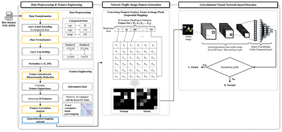
Figure 1. The overall architecture of the proposed malicious network traffic detection framework.

3.1. Feature Engineering Overview

The data preprocessing and feature engineering module converts raw data into image data. This module is structured into two primary components: data preprocessing and feature engineering. In data preprocessing, first, data transformation converts categorical features (non-numeric features) into numeric feature vectors using label encoding as a method. Then, in data normalization, all numeric feature vectors are normalized by applying feature scaling, and all the feature values are converted to values between 0 and 255. If the range of values of a feature varies significantly, biases towards these features can emerge. To address this issue, the logarithmic function is applied for feature scaling. In the feature engineering component, information gain is used to measure the importance of each feature and to reduce the dimensionality complexity of the data. Features with lower importance based on the measured information gain values are discarded, while the remaining features with higher importance are retained. Additionally, feature correlation analysis examines the relationships between features to determine the optimal pixel mapping strategy for image generation. In particular, we tested whether arranging highly correlated features to adjacent pixels in the image improves classification accuracy. However, the experimental results showed no significant performance difference compared to simple sequential pixel mapping; thus, the final feature vectors were arranged in sequential pixel order.

The network traffic image dataset generation module creates an image dataset based on the finalized numeric feature vectors produced by the data preprocessing and feature engineering module. Through sequential pixel mapping, each feature value is assigned to a specific position in a 6 × 6-pixel grid, creating a two-dimensional grayscale image representation of each network traffic sample. Through this process, attack and normal image datasets are generated, respectively.

Finally, the CNN-based detection module utilizes a CNN model designed with parameters optimized through experiments. This module trains a model with the network traffic image dataset generated in the previous processes and measures the classification accuracy of malicious network traffic using a test set. The CNN architecture processes the spatial patterns present in the traffic images, effectively learning to differentiate between normal and malicious network behaviors based on their visual signatures.

3.2. NSL-KDD Dataset Description

To evaluate our framework, we used the NSL-KDD dataset [69], which is widely used for IDS evaluation. This dataset is an enhanced version of the KDD CUP 99 dataset, which was originally developed by the Defense Advanced Research Project Agency (DARPA) for IDS evaluation.

Table 1 and Table 2 show 41 network traffic features and descriptions of each class, as well as the number of data samples per class in the NSL-KDD dataset [70]. Characteristics of the dataset are provided in a csv file format, consisting of 41 feature columns and 1 class column. The class consists of a normal state and four types of attack: Denial of Service (DoS), Remote-to-Local (R2L), User-to-Root (U2R), and Probe. We grouped data samples of the four attack types into one attack class for the experiments. When the class is divided into two types, normal and attack, the dataset is composed of 77,054 normal samples and 71,463 attack samples, among a total of 148,517 data samples.

Table 1. The NSL-KDD dataset feature description.

No.	Feature Name	Description
1	duration	Duration of the connection
2	protocol_type	Connection protocol
3	service	Destination service
4	flag	Status of the connection—Normal or Error
5	src_bytes	Bytes sent from source to destination
6	dst_bytes	Bytes sent from destination to source
7	land	The source and destination IP addresses and port numbers are the same
8	wrong_fragment	Total number of wrong fragments in this connection
9	urgent	Number of urgent packets
10	hot	Number of “hot” indicators
11	num_failed_logins	Count of failed login attempts
12	logged_in	Login Status
13	num_compromised	Number of “compromised” conditions
14	root_shell	A value of 1 if root shell is obtained; 0 otherwise
15	su_attempted	A value of 1 if the ‘su root’ command is attempted or used; 0 otherwise
16	num_root	Number of “root” accesses or number of operations performed as a root in the connection
17	num_file_creations	Number of file creation operations in the connection
18	num_shells	The number of times the shell command is used
19	num_access_files	Number of operations on access control files
20	num_outbound_cmds	Number of outbound commands in an ftp session
21	is_host_login	1 if the login belongs to the “hot” list i.e., root or admin; else 0
22	is_guest_login	1 if the login is a “guest” login; 0 otherwise
23	count	Number of connections to the same destination host
24	srv_count	Number of connections to the same port number service
25	serror_rate	% of connections that have “SYN” errors
26	srv_serror_rate	% of connections that have “SYN” errors
27	rerror_rate	% of connections that have “REJ” errors
28	srv_rerror_rate	% of connections that have “REJ” errors
29	same_srv_rate	% of connections to the same service
30	diff_srv_rate	% of connections to different services
31	srv_diff_host_rate	% of connections to different hosts
32	dst_host_count	Number of connections having the same destination host IP address
33	dst_host_srv_count	Number of connections having the same port number
34	dst_host_same_srv_rate	% of connections having the same destination host and using the same service
35	dst_host_diff_srv_rate	% of different services on the current host
36	dst_host_same_src_port_rate	% of connections to the current host having the same src port
37	dst_host_srv_diff_host_rate	% of connections to the same service coming from different hosts
38	dst_host_serror_rate	% of connections to the current host that have an S0 error
39	dst_host_srv_serror_rate	% of connections to the current host and specified service that have an S0 error
40	dst_host_rerror_rate	% of connections to the current host that have an RST error
41	dst_host_srv_rerror_rate	% of connections to the current host and specified service that have an RST error

Table 2. NSL-KDD dataset class distribution.

Class	Description	# of Samples
Normal	Represents regular, benign activities in the network.	77,054
DoS	Obstructs or disrupts access to a system or network (i.e., “back”, “land”, “neptune”, “pod”, “smurf”, “teardrop”).	53,385
R2L	A remote user attempts to gain local access to a system (i.e., “ftp_write”, “guess_passwd”, “imap”, “multihop”, “phf”, “spy”, “warezclient”, “warezmaster”).	14,077
U2R	A standard user attempts to gain system administrator privileges (i.e., “buffer_overflow”, “loadmodule”, “perl”, “rootkit”).	3749
Probe	Scanning a network or probing a system to discover vulnerabilities (i.e., “ipsweep”, “nmap”, “portsweep”, “satan”).	252

Figure 2 shows the distribution of normal and attack data samples in the NSL-KDD dataset, visualized using t-distributed Stochastic Neighbor Embedding (t-SNE) [71]. t-SNE is a dimensionality-reduction technique that maps high-dimensional feature data into a two-dimensional space while preserving the local structure of data samples, and it is widely used for visualizing and analyzing the distribution of data samples with high-dimensional features. The x and y axes of the t-SNE visualization indicate spatial coordinates in the low-dimensional space without any specific meaning. As shown in Figure 2, the number of normal and attack data samples is nearly equal, confirming that the dataset maintains a balanced class distribution after grouping all attack types into a single class. Maintaining a balanced distribution of normal and attack classes prevents classification bias and improves model generalization by mitigating the impact of class imbalance.

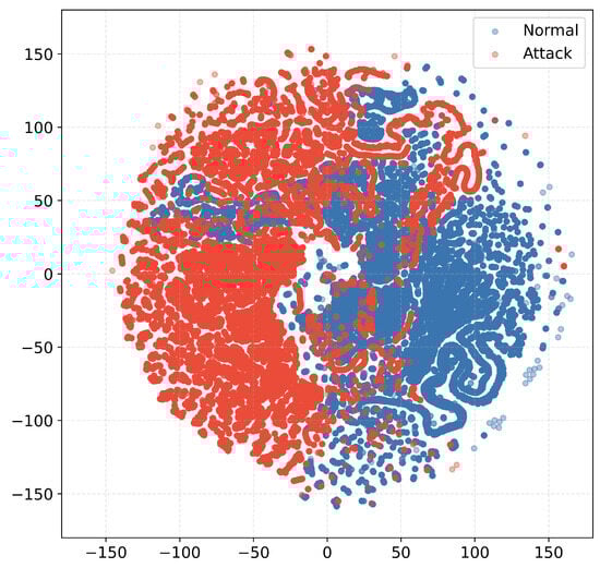
Figure 2. Data distribution visualization by t-SNE.

3.3. Data Preprocessing and Feature Engineering

As shown in Figure 1, the data preprocessing and feature engineering module is divided into two main components: data preprocessing, which converts raw network traffic data into normalized numeric feature vectors, and feature engineering, which refines these vectors by selecting relevant features and analyzing their relationships. These processes are essential to reduce data dimensionality, mitigate biases from varying feature scales, and ultimately generate meaningful image representations for the CNN model. In the data preprocessing component, we first perform data transformation to encode categorical (non-numeric) features into numeric values. Then, data normalization is applied to rescale all feature values to a consistent range. In the feature engineering component, we employ feature selection based on information gain to remove features with low importance, thereby reducing dimensional complexity. Finally, feature correlation analysis examines the relationships between the selected features to determine an optimal pixel mapping strategy for image generation. In the following subsections, each step is explained in detail.

3.3.1. Data Transformation Using Label Encoding for Non-Numeric Data

Data transformation is a critical step in the data preprocessing process, particularly when working with heterogeneous network traffic data that contains both categorical and numerical features. Machine learning algorithms, especially CNN models, require numerical inputs to function properly. Effective transformation strategies not only enable algorithm compatibility but also significantly impact model performance by influencing how the underlying patterns are represented and learned.

In the data transformation step, categorical features must be converted to numerical representations. Two primary encoding approaches are commonly used: one-hot encoding and label encoding, each with distinct characteristics that affect model performance and computational efficiency. The one-hot encoding method is most widely used to convert a categorical feature vector to a numeric feature vector using 0 and 1. For example, the protocol_type feature in the NSL-KDD dataset has three unique values, namely ‘tcp’, ‘udp’, and ‘icmp’, and ‘tcp’ can be represented as (1, 0, 0), ‘udp’ as (0, 1, 0), and ‘icmp’ as (0, 0, 1). This approach preserves the categorical nature of data by maintaining independence between categories, preventing the model from learning false ordinal relationships. However, this method generates new feature vectors in proportion to the number of unique values that the feature has. This can significantly increase the number of feature vectors, which can cause the curse of dimensionality problem, which can lead to performance degradation. The curse of dimensionality refers to various phenomena that arise when analyzing data in high-dimensional spaces. As dimensionality increases, the available data become increasingly sparse, making pattern recognition more difficult. In our image-based approach, one-hot encoding would create unnecessarily large and sparse representations. For instance, the service feature alone contains over 70 unique values, and applying one-hot encoding to all categorical features in the NSL-KDD dataset would result in over 100 additional dimensions, creating highly sparse image representations that hinder the performance of classification models.

To address this dimensionality challenge, we adopted label encoding in our framework. Label encoding directly maps categorical feature values to specific numeric values in a simple manner. The numerical features are then normalized to pixel intensity values ranging from 0 to 255 for image conversion. For example, the protocol_type feature’s three unique values are assigned numerical values of 1, 2, and 3, which are then normalized to 85, 170, and 255, respectively. This encoding method maintains the original feature dimensionality while enabling efficient image-based representation.

However, label encoding introduces potential biases that must be considered. The primary concern is the artificial creation of ordinal relationships among categorical values. The model might incorrectly interpret that ‘udp’ (170) is somehow positioned “between” ‘tcp’ (85) and ‘icmp’ (255) in terms of importance or similarity. Additionally, the numerical spacing between encoded values might be interpreted as meaningful distances, potentially leading to biased learning patterns. These biases are particularly problematic for distance-based algorithms that rely on numerical proximity calculations (e.g., KNN and SVM).

Despite these concerns, our image-based detection approach provides inherent advantages that help mitigate the potential biases introduced by label encoding. First, CNNs primarily learn spatial patterns and local features rather than interpreting individual pixel intensities as ordinal values. The convolutional operations focus on detecting edges, textures, and patterns across spatial neighborhoods, which reduces sensitivity to specific numerical values of individual pixels. This spatial pattern learning mechanism prevents the model from being misled by the artificial ordinal relationships in label encoding. Second, our normalization strategy distributes encoded values across the full pixel intensity range (0–255), ensuring no category is assigned extreme values that might be interpreted as more or less important, thereby maintaining balanced feature representation.

Therefore, since label encoding maintains dimensional efficiency without increasing feature dimensions, and the inherent characteristics of CNN architecture in processing images can preserve the advantages of label encoding while mitigating its disadvantages, label encoding was applied to the data transformation process in this study.

Table 3 shows the results of converting categorical features to numeric features. As shown in the table, each categorical value is mapped to a specific numeric value consistently. The ‘flag’ feature’s 11 unique categorical values are transformed into evenly distributed numeric values between 23 and 253, preserving the distinctiveness of each category. Similarly, the ’service’ feature, with its numerous unique values, is mapped to values starting from 3 and incrementing appropriately, ensuring each service type maintains a unique representation in the generated images. This systematic encoding approach allows the CNN to potentially identify patterns associated with specific network services and flags that may be indicative of malicious traffic.

Table 3. The results of converting categorical features into numeric features.

Feature Name	Categorical Feature	Numeric Feature
protocol_type	tcp	85
	udp	170
	icmp	255
flag	SF	23
	S0	46
	REJ	69
	RSTR	92
	SH	115
	RSTO	138
	S1	161
	RSTOS0	184
	S3	207
	S2	230
	OTH	253
service	ftp_data	3
	other	6
	private	9
	http	12
	remote_job	15
	name	18
	netbios_ns	21
	eco_i	24
	mtp	27
	telnet	30
	…	…
	netbios_ssn	186
	rje	189
	X11	192
	urh_i	195
	http_8001	198
	aol	201
	http_2784	204
	tftp_u	207
	harvest	210

3.3.2. Data Normalization

In the previous data transformation step, categorical features were converted into numeric feature vectors using label encoding. However, the numeric feature vectors in the NSL-KDD dataset exhibit different ranges and scales, which can cause biased or inefficient learning in CNN models if used directly. For instance, certain features such as packet sizes or byte counts typically have extremely large and skewed value distributions, potentially dominating the learning process. Thus, data normalization is an essential step to align the numeric features into a consistent and standardized scale.

The NSL-KDD dataset includes numeric feature vector types of integer, float, and binary. For integer and float types of feature values, the logarithm function is applied, as shown in Equation (1). Then, it is normalized to the range from 0 to 255 to match the intensity range of grayscale image pixels.

$$\begin{array}{c}\hfill x_{\mathrm{scaled}}=log\left(x_i\right)\end{array}$$

(1)

This normalization range corresponds directly to the standard grayscale image pixel value range (0–255), enabling a direct and natural transformation from features to image representation. In this study, logarithmic scaling is used instead of Min–Max or Z-score normalization, as it offers several advantages in handling the characteristics of network traffic data. Logarithmic transformation effectively handles the large value ranges and skewed distributions commonly found in network traffic features such as byte counts and packet sizes. Unlike linear scaling methods, logarithmic transformation better preserves the relative differences between smaller values while compressing the effect of outliers and extreme values, which are common in network traffic due to sporadic bursts or anomalous behaviors.

Figure 3 shows the results before and after feature scaling for the src_bytes and dst_bytes features, which have high IG values.

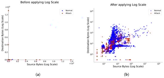
Figure 3. The results before and after feature value normalization. (a) Data distribution before applying log scaling. (b) Data distribution after applying log scaling.

Binary-type feature values are composed of two values, 0 or 1; here, 0 is not converted, and 1 is converted to 255. This binary conversion ensures maximum contrast between the presence (255) and absence (0) of binary features in the generated grayscale image, making these patterns more distinguishable for the CNN model.

Before applying feature scaling, the two features have different scales, which is shown in Figure 3a. After applying feature scaling, however, the data samples are shown to be distributed within a similar scale, which indicates that the ratio of distances between samples is well-balanced and there is no bias towards a particular feature.

The logarithmic transformation particularly benefits features like src_bytes and dst_bytes, which typically exhibit exponential or power-law distributions in network traffic. As shown in Figure 3b, after applying log scaling, previously imperceptible differences between smaller values become more distinguishable, while extremely large values no longer dominate the feature space. This balanced representation prevents the CNN from overemphasizing features with naturally larger numerical ranges and ensures that all relevant patterns contribute proportionally to the learning process.

3.3.3. Information Gain-Based Feature Selection

Commonly used feature selection methods include wrapper-based methods, embedded methods, and filter-based methods [72]. Wrapper methods select features based on specific classifier performance, making them computationally expensive. Embedded methods perform feature selection during the model training process, but they are model-specific and can lack flexibility. On the other hand, filter-based methods, such as information gain, independently evaluate feature importance regardless of any specific classification algorithm, thus providing greater flexibility and lower computational cost [73]. Moreover, filter-based methods generally offer significantly lower computational complexity and stronger robustness against overfitting compared to wrapper and embedded methods [74]. In particular, information gain ranks features based on entropy, effectively identifying informative attributes and eliminating irrelevant ones. These characteristics make information gain especially suitable for anomaly detection tasks involving high-dimensional datasets. Thus, information gain was chosen as the dimensionality reduction method for the feature selection step in this study to address the curse of dimensionality problem [75,76].

After measuring the information gain value for each feature, the dimensionality is reduced by removing features with relatively low information gain values. To calculate information gain, the entropy of the dataset must first be quantified. Entropy is a fundamental concept from information theory, representing data uncertainty and the uniformity of distribution within a dataset. Higher entropy indicates greater diversity among samples, while lower entropy indicates more similarity.

The main equations for information gain and entropy are as follows [77]:

$$\begin{array}{c}\hfill H\left(S\right)=-\sum _{i=1}^n{p}_i{log}_2{p}_i\end{array}$$

(2)

$$\begin{array}{c}\hfill H\left(S\right|F)=-\sum _{i=1}^m{p}_{i}H\left(S\right|F=f_i)\end{array}$$

(3)

$$\begin{array}{c}\hfill I.G(S,F)=H\left(S\right)-H\left(S\right|F)\end{array}$$

(4)

where S denotes the set of data samples, and F denotes the set of features of data samples. $H\left(S\right)$ denotes the entropy of dataset S. n denotes the number of classes of dataset, and $p_i$ denotes the ratio of data belonging to class i in dataset S.

Equation (3) calculates the conditional entropy of dataset S given feature set F. The result value indicates how well the data is distinguished by the feature set F. By using Equations (2) and (3), the information gain of each feature can be calculated. Table 4 shows the information gain (IG) values for 41 features of the NSL-KDD dataset. The information gain values were calculated using the Weka InfoGainAttributeEval API [78]. A larger value indicates a higher importance of the feature. As shown in Table 4, src_bytes has the largest value among the features, which means that the feature can distinguish malicious and benign traffic most effectively. Conversely, features such as num_outbound_cmds, num_shells, and urgent have IG values of 0, indicating these features provide no discriminative information for classification.

Table 4. The information gain values of Nsl-Kdd features.

Rank	Feature Name	I.G Value
1	src_bytes	0.7814411
2	dst_bytes	0.6248539
3	service	0.6197358
4	flag	0.4727718
5	diff_srv_rate	0.4604546
6	same_srv_rate	0.4500181
7	dst_host_srv_count	0.4269103
8	dst_host_same_srv_rate	0.3909421
9	dst_host_diff_srv_rate	0.3721759
10	logged_in	0.3601069
11	count	0.3390986
12	dst_host_serror_rate	0.3373162
13	serror_rate	0.3313643
14	dst_host_srv_serror_rate	0.3287723
15	srv_serror_rate	0.3114433
16	dst_host_srv_diff_host_rate	0.2479778
17	dst_host_count	0.1850297
18	dst_host_same_src_port_rate	0.1840325
19	srv_diff_host_rate	0.1400392
20	dst_host_srv_rerror_rate	0.0910595
21	rerror_rate	0.0786418
22	dst_host_rerror_rate	0.0767992
23	srv_rerror_rate	0.0715524
24	srv_count	0.0687273
25	protocol_type	0.0581388
26	duration	0.0342559
27	hot	0.0148091
28	num_compromised	0.007111
29	wrong_fragment	0.0063851
30	num_root	0.0025104
31	num_failed_logins	0.0023726
32	num_access_files	0.0017842
33	num_file_creations	0.0006682
34	su_attempted	0.0004711
35	root_shell	0.0001348
36	land	0.000059
37	is_host_login	0.0000511
38	is_guest_login	0.0000106
39	num_outbound_cmds	0
40	num_shells	0
41	urgent	0

The information gain results on the NSL-KDD dataset reveal that traffic volume features (src_bytes and dst_bytes) and connection behavior features (service and flag) provide the most discriminative power. This aligns with known attack signatures, where abnormal data transfer sizes and unusual service usage patterns often indicate malicious activity. Features with IG values near zero contribute negligible information for classification, and their removal reduces noise while improving computational efficiency. We removed the bottom five features with the smallest IG values to reduce the number of data dimensions, resulting in the remaining 36 features. The reason why we selected 36 features is to convert the final generated feature vector to a 6 × 6 square image with 36 pixels through the data preprocessing process.

Algorithm 1 summarizes the overall process of the data preprocessing and feature engineering module. This systematic preprocessing pipeline includes categorical feature transformation using label encoding to prevent dimensionality expansion, logarithmic normalization to mitigate bias from varying feature scales, and dimensionality reduction via information gain-based feature selection. As a result, the raw NSL-KDD dataset is effectively converted into a compact and informative 36-dimensional numeric feature vector optimized for subsequent grayscale image generation.

3.3.4. Feature Correlation Analysis

CNN models process and analyze data by taking into account the spatial locality and relationships between adjacent pixels [79]. Consequently, the spatial arrangement of features when generating images from numeric feature vectors may influence CNN classification performance. Therefore, we conducted a correlation analysis to determine whether arranging highly correlated features adjacent to each other in the image would improve classification accuracy.

Algorithm 1 Data Preprocessing & Feature Engineering Algorithm
Input: Raw Dataset (NSL-KDD) Output: 36 Preprocessed features for image conversion
1: $F\leftarrow$ All features from Raw Dataset
2: $D\leftarrow$ DataFrame containing all features from Raw Dataset
3: /* Data Transformation */
4: for each $col$ in $D.columns$ do
5:     if $col.dtype$ == categorical then
6:          $D\left[col\right]\leftarrow LabelEncoder\left(D\right[col\left]\right)$	▹ e.g., ‘tcp’ → 85, ‘udp’ → 175, ‘icmp’ → 255
7:     end if
8: end for
9: /* Data Normalization */
10: for each $col$ in $D.columns$ do
11:     if $col.dtype$ == integer or float then
12:          $D\left[col\right]\leftarrow np.trunc(np.log(D\left[col\right]\left)\right)$	▹ Apply Log Scaling
13:          $D\left[col\right]\leftarrow ScaleToRange\left(D\right[col],0,255)$	▹ Normalize to [0, 255]
14:     else if $col.dtype$ == binary then
15:          $D.loc\left[D\right[col]==1,col]=255$	▹ Map binary 1 to 255
16:          $D.loc\left[D\right[col]==0,col]=0$	▹ Map binary 0 to 0
17:     end if
18: end for
19: /* Feature Selection for Dimensionality Reduction */
20: Calculate Information Gain for all features in D
21: $F_{\mathrm{selected}}\leftarrow$ Top 36 features with highest Information Gain
22: $D_{\mathrm{reduced}}\leftarrow$ DataFrame containing only features in $F_{\mathrm{selected}}$
23: return $D_{\mathrm{reduced}}$	▹ 36 preprocessed features as feature vector $\{F_1,F_2,F_3,\dots ,F_{36}\}$

Specifically, to analyze the relationships between all feature vectors, we utilized the Pearson Correlation Coefficient (PCC) [80,81,82], calculating correlation coefficients through Equation (5) to generate a correlation matrix. Based on this matrix, we tested a correlation-based pixel mapping method, where features with high correlation values were positioned adjacently within the generated 6 × 6 pixel image.

$$r_{xy}={\displaystyle \frac{{\sum }_{i=1}^n(x_i-\overline{x})(y_i-\overline{y})}{\sqrt{{\sum }_{i=1}^n{(x_i-\overline{x})}^2}\sqrt{{\sum }_{i=1}^n{(y_i-\overline{y})}^2}}}$$

(5)

where $r_{xy}$ represents the PCC between features x and y, $x_i$ and $y_i$ are the feature values of the i-th sample, $\overline{x}$ and $\overline{y}$ denote the mean values of each feature, and n is the number of samples.

Figure 4 displays a heatmap matrix of the correlation analysis for the 41 features, while Table 5 shows the results of the calculated correlation coefficients. The correlation analysis revealed that the relationship between serror_rate and srv_serror_rate has the highest correlation coefficient (0.9915), while the correlation between count and same_srv_rate is the lowest (−0.7336). As shown in Figure 4, features with high correlations are represented in deep red, while those with low correlations appear in deep blue. The diagonal elements showing self-correlation are represented by the deepest red color, indicating a perfect correlation of 1.0. Table 5 confirms these findings by listing the top five highest positive correlations and the five lowest negative correlations among the features. To examine the impact of feature correlation on classification performance, we conducted comparison experiments between correlation-based and sequential pixel mapping strategies, as described in Section 4.2. These experiments revealed negligible differences in CNN classification accuracy between these approaches. Therefore, to maintain simplicity and computational efficiency, we ultimately adopted sequential mapping of feature vectors into image pixels for the final dataset generation.

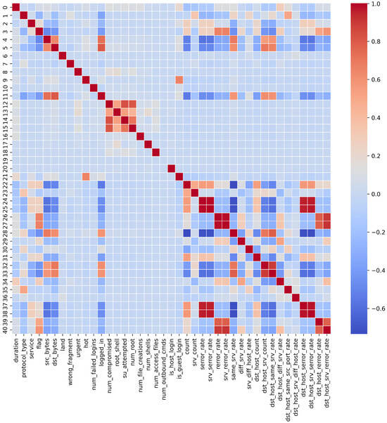
Figure 4. Correlation heatmap of NSL-KDD dataset features.

Table 5. Correlation coefficient of features.

Feature 1	Feature 2	Correlation Coefficient
serror_rate	srv_serror_rate	0.991513873
rerror_rate	srv_rerror_rate	0.986079836
dst_host_serror_rate	dst_host_srv_serror_rate	0.973556272
srv_serror_rate	dst_host_srv_serror_rate	0.970102601
serror_rate	dst_host_srv_serror_rate	0.964217993
…	…	…
srv_serror_rate	same_srv_rate	−0.707400373
serror_rate	same_srv_rate	−0.711250693
same_srv_rate	dst_host_serror_rate	−0.717951623
same_srv_rate	dst_host_srv_serror_rate	−0.726708916
count	same_srv_rate	−0.733642863

3.4. Image Dataset Generation

The image dataset generation module converts a numeric feature vector into an image dataset. As shown in Figure 1, 36 feature values are stored sequentially in each pixel of a 6 × 6, two-dimensional grayscale image. Consequently, a total of 148,517 images are generated, with 77,054 normal packets and 71,463 attack packets. The reasons why we employed a method that sequentially stores each feature value as an individual pixel in the image generation process are explained in Section 4.

3.5. Designing a CNN-Based Malicious Network Traffic Detection Model

A CNN model was designed to classify the network traffic images generated through data preprocessing and network traffic image generation modules into normal and attack. CNN models have shown excellent performance in the field of computer vision, especially in image classification tasks [83].

One of the main advantages of CNN models is that they can capture patterns to distinguish different kinds of images. CNN models can reflect spatial information in images and the correlation between adjacent pixels. Such capability enables the models to achieve high classification accuracy when there is a strong association among the pixels in an image. Converting network traffic packets to image data for analysis makes it easier to identify patterns of malicious network traffic packets that appear in specific areas of the image.

Correlations exist among the features of the NSL-KDD dataset [84]. Therefore, converting each feature from the NSL-KDD dataset into pixels of an image and training a CNN model with these data enable image classification leveraging spatial information among adjacent pixels.

Figure 5 shows the structure of our CNN model, represented in the LeNet-5 architecture [83], and Table 6 shows the parameters of the model. To adjust hyperparameters, such as the number of layers, batch size, and filter size, different models were designed, and multiple experiments were conducted to find the model with the highest classification accuracy. While deeper networks with more layers can potentially learn more complex patterns, they also risk overfitting, especially with limited data dimensions like our 6 × 6 images, and increase the computational cost; conversely, shallower networks might underfit. Our experiments indicated that the current architecture with two convolutional and two max-pooling layers (as shown in Figure 5) provided the best trade-off, achieving high accuracy for this specific task.

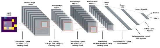
Figure 5. Our CNN model architecture.

Table 6. The parameters of our CNN model.

Layer	Output	Activation	# of Weights
Input	6, 6, 1		0
Conv2D_1	6, 6, 32	ReLU	320
MaxPool2D_1	3, 3, 32	-	0
Conv2D_2	3, 3, 64	ReLU	18,496
MaxPool2D_2	2, 2, 64	-	0
Flatten	256	-	0
Dense1	128	ReLU	32,896
Dense2	1	Sigmoid	129

After the initial input layer, two Conv2D layers use 32 and 64 filters, respectively, with a size of 3 and a stride of 1. Regarding the number of filters, using too few might fail to capture sufficient features from the input image, whereas using too many significantly increases the number of parameters and the risk of overfitting. We adopted the commonly used filter counts of 32 and 64, which experimental results confirmed were effective for extracting relevant patterns from our 6 × 6 grayscale images without excessive complexity. The Rectified Linear Unit (ReLU) [85] was used as the activation function.

The max-pooling layer takes the output of the Conv2D layer as input, with a specified pooling size of 2. The resulting feature map is then transformed into a one-dimensional vector by the flatten layer. This vector subsequently passes through two fully connected layers with 256 and 128 neurons, respectively. Finally, the probability value is calculated using the $sigmoid$ function to classify whether the image represents a normal or attack state. In both the Conv2D layers and the max pooling layers, zero padding was employed to minimize the loss of image information.

After adjusting batch sizes in several experiments with different sizes, a batch size of 32 consistently achieved the highest classification accuracy and the lowest loss. Lastly, to find the optimal learning rate for the model, we used the TensorFlow learning rate scheduler, which provides the functionality to dynamically fine-tune the learning rate. By setting the learning rate between 0.001 and 0.00001 and conducting model training experiments, we observed that the highest performance was achieved at a learning rate of 0.0001. When the learning rate was smaller than 0.0001, the loss converged slowly, resulting in decreased training speed. Conversely, when the learning rate was larger than 0.001, the loss diverged, leading to degraded model performance.

The parameter update optimizer used Adaptive Moment Estimation (Adam) [86], which provides a fast learning speed by quickly converging to the global minimum. The final output layer used the $sigmoid$ function, as shown in Equation (6), for binary classification.

$$\widehat{y}=\sigma \left(z\right)={\displaystyle \frac{1}{1+e^{-z}}}$$

(6)

$$\left\{\begin{array}{cc}1\hfill & \mathrm{if}\widehat{y}\ge 0.5,\left(\mathrm{Attack}\right)\hfill \\ 0\hfill & \mathrm{if}\widehat{y}<0.5,\left(\mathrm{Normal}\right)\hfill \end{array}\right.$$

(7)

where z denotes the value of the input image just before it is passed to the final output layer after passing through the network. This value is processed by the $sigmoid$ function, outputting a probability value, $\widehat{y}$, between 0 and 1.

As shown in Equation (7), if the value is 0.5 or higher, the packet is classified as an attack; if the value is less than 0.5, the packet is classified as normal. Binary cross-entropy is used for parameter updates, as calculated in Equation (8). During model training, weights are adjusted to minimize the difference between the ground truth value and the predicted value.

$$L(y,\widehat{y})=-{\displaystyle \frac{1}{N}}\sum _{i=1}^N{y}_{i}log\left(\widehat{y_i}\right)+(1-y_i)log(1-\widehat{y_i})$$

(8)

where y denotes the ground truth, while $\widehat{y}$ signifies the predicted value.

4. Experimental Results

4.1. Experimental Environments

The experiments were conducted on a Windows 11 machine with an Intel Core i7-11700 CPU, a GeForce GTX 1660Ti GPU, and 32GB of RAM. The data preprocessing module was implemented using Anaconda, an open-source data science platform that provides convenient management of various data analysis and preprocessing packages through virtual environments. The CNN model was implemented using TensorFlow [87]. Table 7 shows the detailed experimental environments. To promote reproducible research, we have released our source code publicly on GitHub [88].

Table 7. Experimental environment.

OS and Hardware	OS	Windows 11
	CPU	Intel Core i7-11700
	RAM	32GB
	GPU	NVIDIA GTX 1660Ti
	CUDA Toolkit	NVIDIA CUDA Toolkit 12.2
	cuDNN	NVIDIA cuDNN 12.1.66
Software Libraries	anaconda	4.12.0
	python	3.9.0
	jupyter Lab	4.0.3
	pandas	1.5.3
	tensorflow	2.10.1
	keras	2.10.0
	wandb	0.15.5
	scikit-learn	1.2.1
	weka	3.8.6

4.2. Comparative Analysis of Feature Correlation-Based and Sequential Pixel Mapping

This section explains the reasons for employing a method of sequentially representing each feature value at individual pixels in the image generation process. As mentioned in Section 3.3.4, CNN models perform computations considering spatial correlations, specifically the adjacency of pixels during image processing. To examine the impact of such correlations on image generation, we conducted comparative experiments between correlation-based pixel mapping and sequential pixel mapping strategies.

Figure 6 illustrates the comparison between models trained on images with consideration of feature correlation and models trained without such consideration. The blue curve represents the model trained with correlated features, while the red curve denotes the model trained without considering feature correlation. Solid lines in the graph indicate results from the training set, whereas dashed lines represent results from the validation set. Analysis of the accuracy graph (Figure 6a) and the loss graph (Figure 6b) suggests that feature correlation does not significantly impact model performance. As evidenced by the measured values in Table 8, the differences were found to be minimal. More specifically, the model trained with correlated features achieved an accuracy and validation accuracy of 99.59% and 99.09%, respectively. In contrast, the model without correlation consideration achieved 99.44% accuracy and 98.98% validation accuracy. The difference between these models is merely 0.15% for training accuracy and 0.11% for validation accuracy. Similarly, the difference in loss metrics was negligible (0.0028 for training loss and 0.0024 for validation loss). These minimal differences fall within typical statistical variance ranges for neural network training, indicating no practically significant advantage for correlation-based pixel arrangement. As shown in Figure 6a,b, both models converge to similar performance levels after approximately 40 epochs, with the correlation-based model showing only marginally better results. This marginal performance difference results from two key factors. First, the information gain-based feature selection prioritized individually discriminative features, reducing the additional benefits of correlation-based spatial arrangements. Second, the convolution operations of CNN effectively capture feature interactions regardless of pixel positioning within our compact 6 × 6 image representation.

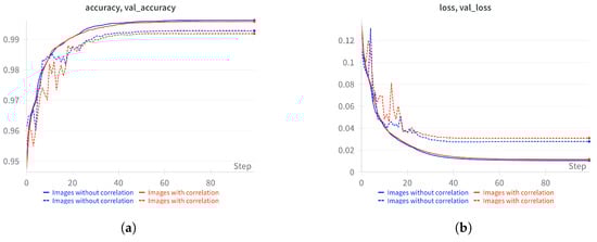
Figure 6. Comparative analysis of model performance trained on images with and without feature correlation. (a) Training and validation accuracy graph for models trained on images with and without feature correlation; (b) training and validation loss graph for models trained on images with and without feature correlation.

Table 8. Comparison of model training results for images with correlation considered and images without correlation consideration.

Images	Accuracy (%)	Validation Accuracy (%)	Loss	Validation Loss
With feature correlation	99.59	99.09	0.0115	0.0309
Without feature correlation	99.44	98.98	0.0143	0.0333

This experiment verifies that feature correlation has a minimal effect on the classification accuracy performance of the model. Therefore, an image generation method was employed that sequentially maps each feature to a single pixel, prioritizing simplicity and computational efficiency. This choice provides equivalent classification performance while significantly reducing the computational overhead associated with measuring inter-feature correlations and subsequent correlation-based pixel mapping during preprocessing.

4.3. The Results of CNN Model Training

To evaluate the classification performance of our proposed model, the generated image dataset of 148,517 images was divided into three sets: a training set (60%), a validation set (20%), and a test set (20%). The model was trained using the training set, and the validation set was utilized for verifying classification accuracy performance and tuning hyperparameters. Finally, the test set was employed to evaluate the model’s generalization performance. When a model is trained, the choice of weight initialization method is an important factor, as it determines the outcome of the model training. TensorFlow offers various weight initialization methods, including Glorot initialization [89] and He initialization [90]. In this study, we used the Glorot initialization method, which initializes weights randomly, and as a result, the model training results can vary each time. Therefore, we measured the model training results a total of 10 times and calculated the average value as the final classification performance of the model.

Figure 7 shows the results of 10 model training runs. Each training run was performed for a total of 100 epochs with a batch size of 32 and a learning rate of 0.0001. The average accuracy was 99.46%, and the val_accuracy was 99.09%, indicating excellent classification performance. During the 100 epochs, the average loss and val_loss converged to 0.0139 and 0.041, respectively, but the val_loss tended to diverge again after the 60th epoch. To evaluate the classification accuracy performance of the model, we used a confusion matrix.

$$\mathrm{Accuracy}={\displaystyle \frac{TP+TN}{TP+TN+FP+FN}}$$

(9)

$$\mathrm{Precision}={\displaystyle \frac{TP}{TP+FP}}$$

(10)

$$\mathrm{Recall}={\displaystyle \frac{TP}{TP+FN}}$$

(11)

$$\mathrm{F-score}={\displaystyle \frac{2\times \mathrm{Precision}\times \mathrm{Recall}}{\mathrm{Precision}+\mathrm{Recall}}}$$

(12)

$$\mathrm{False}\mathrm{Positive}\mathrm{Rate}={\displaystyle \frac{FP}{FP+TN}}$$

(13)

$$\mathrm{False}\mathrm{Negative}\mathrm{Rate}={\displaystyle \frac{FN}{FN+TP}}$$

(14)

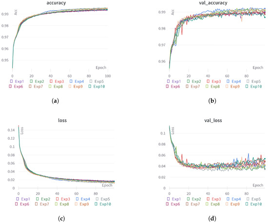
Figure 7. The results of model training accuracy and loss. (a) Training accuracy; (b) validation accuracy; (c) training loss; (d) validation loss.

Detailing the terms within this matrix, True Positive (TP) refers to the accurate classification of attack samples as attack, and True Negative (TN) denotes the correct classification of normal samples as normal. On the other hand, False Positive (FP) signifies the misclassification of normal samples as attack, and False Negative (FN) indicates the misclassification of attack samples as normal. These four metrics constitute the confusion matrix, with performance being measured using Equations (9)–(14). Figure 8 and Table 9 display the confusion matrix and evaluation metric results, respectively.

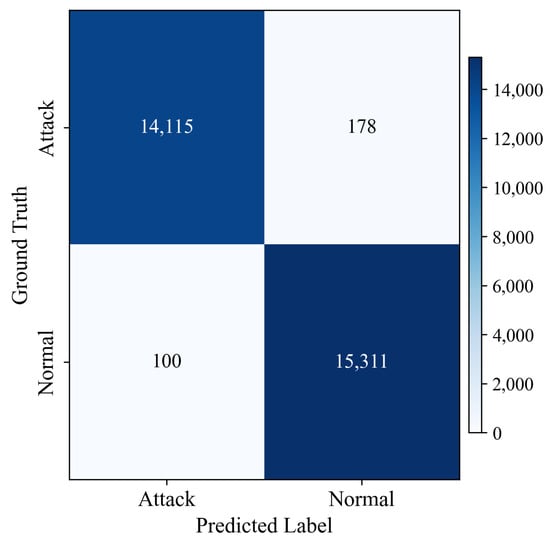
Figure 8. The confusion matrix for binary classification.

Table 9. The results of evaluation metrics.

Precision	Recall	F1-Score	FPR (%)	FNR (%)	Accuracy (%)
0.9875	0.9930	0.9902	0.65	1.25	99.06

The model’s generalization performance was evaluated using the test set. Based on the confusion matrix shown in Figure 9 (TP = 14,115, FN = 178, FP = 100, and TN = 15,311), the precision, recall, F1-score, and accuracy were 0.9930, 0.9875, 0.9902, and 99.06%, respectively. Furthermore, the proposed model achieved a false positive rate (FPR) of 0.65% and a false negative rate (FNR) of 1.25%. The FPR represents the proportion of normal traffic incorrectly classified as attacks, which can lead to alert fatigue and increased operational overhead for security analysts in production environments. Conversely, the FNR indicates the proportion of actual attacks misclassified as normal traffic, which poses more severe security risks as these attacks would go undetected. It is noteworthy that this FNR of 1.25% was obtained from a balanced dataset with approximately a 5:5 ratio of normal to malicious samples. In real-world network environments where normal traffic constitutes the vast majority of total traffic, while the FNR percentage is expected to remain similar, the absolute number of missed attacks would be significantly lower due to the substantially reduced volume of actual attack traffic compared to our test conditions. Our model demonstrates excellent performance with both low false positive and relatively low false negative rates, representing an effective balance between minimizing alert fatigue and maintaining comprehensive attack detection capabilities.

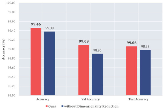
Figure 9. The comparison with models without dimensionality reduction.

4.4. Effectiveness of Feature Engineering

To evaluate the effectiveness of dimensionality reduction in improving a model’s training efficiency, we conducted comparison experiments between two models: one trained on images without dimensionality reduction and the other trained on images with dimensionality reduction. Images without dimensionality reduction were created using one-hot encoding during data preprocessing, so 84 new one-hot encoding features were created by adding the number of unique values of categorical features protocol_type, service, and flag, which are 3, 70, and 11, respectively. When the newly created features are added to the existing 38 numeric features, a total of 122 features are created. To convert it to a square image, we removed the urgent feature, which had the lowest importance, to create an 11 × 11-pixel image based on a total of 121 features. The image dataset generated in this way was trained using our designed CNN model.

Our model uses only 6 × 6-pixel images in comparison to 11 × 11-pixel images with the one-hot encoding method. However, as can be seen in Figure 9, our model has higher accuracy as well as less training time.

While Figure 9 and Figure 10 summarize the overall performance advantages of our approach in terms of accuracy and training time reduction, a more detailed statistical analysis is needed to verify the consistency of these improvements. To comprehensively evaluate the consistency and reliability of our results, each model was trained and tested 10 times. Figure 11 presents the boxplots showing the distribution of performance metrics across these 10 experimental runs. Table 10 summarizes the mean and standard deviation values for each metric. As shown in Table 10, our proposed model with dimensionality reduction consistently outperforms the dimensionality-reduction-free model across all metrics. Not only does it achieve higher average accuracy in training (0.9946 ± 0.00051), validation (0.9909 ± 0.00101), and testing (0.9906 ± 0.00099) compared to the model without feature reduction (0.9938 ± 0.00080, 0.9890 ± 0.00140, and 0.9898 ± 0.00116, respectively), but it also demonstrates greater stability with lower standard deviations in most metrics. The boxplots in Figure 11 visually confirm this trend, showing tighter distributions for the model with feature reduction.

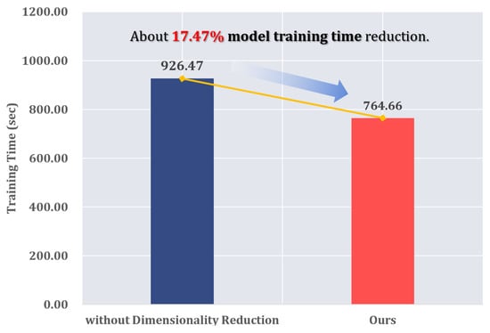
Figure 10. The comparison of model training time.

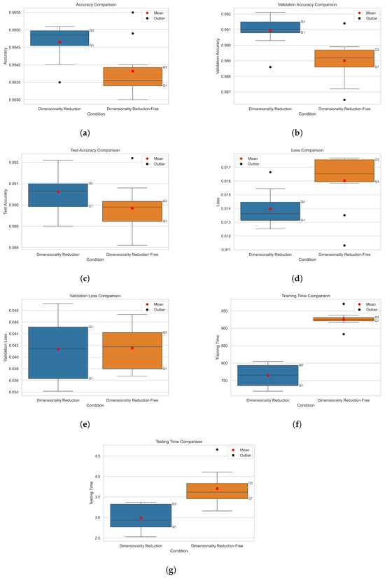
Figure 11. Boxplots comparing performance metrics across 10 experimental runs for models with and without dimensionality reduction. (a) Accuracy; (b) Validation Accuracy; (c) Test Accuracy; (d) Training Loss; (e) Validation Loss; (f) Training Time; (g) Testing Time.

Table 10. Mean and standard deviation of model performance metrics (10 runs).

Metric	Dimensionality Reduction (Mean ± Std)	Dimensionality Reduction-Free (Mean ± Std)
Accuracy (Train)	0.9946 ± 0.00051	0.9938 ± 0.00080
Accuracy (Validation)	0.9909 ± 0.00101	0.9890 ± 0.00140
Accuracy (Test)	0.9906 ± 0.00099	0.9898 ± 0.00116
Loss (Train)	0.01397 ± 0.00128	0.01604 ± 0.00209
Loss (Validation)	0.04132 ± 0.00542	0.04154 ± 0.00384
Training Time (s)	764.66 ± 32.53	926.47 ± 21.34
Testing Time (s)	2.99 ± 0.33	3.71 ± 0.43

Note: The unit “s” denotes seconds.

Similarly, the loss metrics indicate better performance for our proposed model, with a training loss of 0.01397 ± 0.00128 compared to 0.01604 ± 0.00209 for the model without dimensionality reduction, as seen in Table 10. The validation loss shows a similar pattern (0.04132 ± 0.00542 vs. 0.04154 ± 0.00384), though with slightly higher variability in our model.

Figure 10 shows the model training time of the proposed model in comparison to the model without dimensionality reduction. As presented in Table 10 and visualized in Figure 11, the average training time for the model without dimensionality reduction was 926.47 ± 21.34 s, while our model was trained in an average of 764.66 ± 32.53 s. This result shows that our model was trained about 17.47% faster and that the image dataset generated using one-hot encoding consumes relatively much more time for model training.

On the other hand, the testing time was measured based on the test set used to evaluate the prediction performance of the trained model. As shown in Table 10, the dimensionality-reduction-free model took an average of 3.71 ± 0.43 s, whereas the proposed model completed the evaluation in an average of 2.99 ± 0.33 s, achieving a 19.44% improvement in inference speed. These results confirm that the proposed framework improved the speed and efficiency of normal and attack classification predictions while minimizing resource consumption through the application of dimensionality reduction. The small standard deviations observed across accuracy measurements ($\sigma \le 0.0014$), loss metrics, training times, and inference times indicate that the performance improvements are consistent and not due to random variations in model initialization. The boxplots further demonstrate that even in experimental runs with the lowest observed performance (worst-case scenarios), our model with dimensionality reduction consistently outperforms the dimensionality-reduction-free model across most metrics.

In conclusion, the proposed framework showed high classification accuracy and fast model training and testing time. These results demonstrate that the framework can achieve significant performance improvement in real-time malicious network traffic detection in IDSs.

To comprehensively evaluate our dimensionality reduction approach, we compared our framework with existing studies that employed various dimensionality reduction techniques on intrusion detection datasets, as summarized in Table 11.

Table 11. Comparison with existing IDS studies applying dimensionality reduction.

Study	Dataset	Method	Dim. (Before→ After)	Red. (%)	Model	Acc. Before	Acc. After	Acc. $\Delta$	Train Time Before	Train Time After	Train Time $\Delta$ (%)	Infer. Time Before	Infer. Time After	Infer. Time $\Delta$ (%)
Ours	NSL-KDD	InfoGain	41 → 36	12.2	CNN	98.98	99.06	+0.08	926	764	+17.47	3.71	2.99	+19.44
[54]	NSL-KDD	Autoencoder	41 → 10	75.6	Extra Trees	99.40	99.20	$-0.20$	-	-	-	-	-	-
[62]	NSL-KDD	LNNLS-KH	122 → 7	94.3	KNN	91.22	96.12	+4.90	3574.7	4171.8	$-16.7$	41.35	34.38	+16.8
[55]	NSL-KDD	PCA-ADASYN	121 → 28	76.9	ResInceptNet-SA	94.20	99.34	+5.14	-	-	-	11.6	9.8	+15.5
[58]	NSL-KDD	PCA	41 → 7	82.9	Naïve Bayes	77.50	80.60	+4.10	86.7	396.5	$-357.7$	-	-	-
[60]	NSL-KDD	mRMR	39 → 10	75.4	MLP	85.73	85.73	0.00	207.3	141.3	+31.8	8.1	5.9	+27.2
[66]	UNSW-NB15	InfoGain	52 → 20	61.5	DT	88.40	88.14	$-0.26$	-	-	-	-	-	-
[61]	UNSW-NB15	ReliefF	73 → 9	87.7	LR	86.10	86.10	0.00	74.7	89.3	$-19.5$	-	-	-
[68]	CICIDS2017	PCA	78 → 10	87.2	CNN	97.50	97.20	$-0.30$	-	-	+80.0	18.0	6.0	+66.7
[59]	CICIDS2017	PCA	100 → 51	49.0	DT	98.60	98.60	0.00	-	-	-	-	-	-

Note: Dim. (Before→After): Number of features before and after reduction; Red. (%): Dimensionality reduction ratio; Acc. $\Delta$ (%): Absolute change in accuracy (Accuracy_After–Accuracy_Before); Train Time, $\Delta$ (%): Relative change in training time; Infer. Time $\Delta$ (%): Relative change in inference time. ‘+’ indicates improvement; ‘−’ indicates degradation. References: Moyano et al., 2023 [54]; Li et al., 2021 [62]; Liu et al., 2025 [55]; Obeidat et al., 2022 [58]; Wu et al., 2020 [60]; Awad et al., 2023 [66]; Abdulhammed et al., 2019 [61]; Chen et al., 2024 [68]; Mishra et al., 2020 [59].

Our approach demonstrates several notable advantages when considering the holistic trade-offs between dimensionality reduction extent, accuracy, and computational efficiency. First, a key strength of our approach is achieving superior classification accuracy (99.06%) with only minimal dimensionality reduction (12.2%, from 41 to 36 features, as shown in the ‘Red. (%)’ column). This minimal reduction, unlike studies applying substantial feature reduction (ranging from 49.0% to 94.3% in Table 11), prioritizes preserving the original information content. This strategic feature selection contributed to our model’s high accuracy (99.06%), which outperformed other NSL-KDD-based approaches, such as those of Li et al. [62] (96.12%), Obeidat et al. [58] (80.60%), and Wu et al. [60] (85.73%) in terms of ‘Acc. After’. Furthermore, another significant strength is the balanced improvement across multiple performance facets: our framework exhibits substantial reductions in both training time (approx. 17.47%; ‘Train Time $\Delta$ (%)’) and inference time (approx. 19.44%; ‘Infer. Time $\Delta$ (%)’) while simultaneously maintaining, and even slightly improving, classification accuracy (+0.08% ‘Acc. $\Delta$’). This positive ‘Acc. $\Delta$’ contrasts sharply with the weaknesses observed in several other approaches where accuracy degradation was a notable trade-off. For instance, studies by Moyano et al. [54], Awad et al. [66], and Chen et al. [68] reported accuracy degradations (‘Acc. $\Delta$’ values of −0.20%, −0.26%, and −0.30%, respectively) after applying their DR techniques.

Regarding computational efficiency, while our method shows significant improvements, some studies present different trade-off profiles. For example, Li et al. [62] and Obeidat et al. [58] experienced considerably increased training times (indicated by negative ‘Train Time $\Delta$ (%)’ values of −16.7% and −357.7%, respectively, where ‘−’ signifies degradation, as per Table 11 note), despite reducing features, highlighting a critical inefficiency in their post-DR modeling or the DR process itself. In contrast, our positive ‘Train Time $\Delta$ (%)’ of +17.47% underscores our efficiency gain. Although Wu et al. [60] achieved higher percentage improvements in training time (+31.8%) and inference time (+27.2%) compared to our approach, their significant trade-off was a considerably lower overall accuracy (85.73% ‘Acc. After’) post-DR, whereas our method achieved 99.06%. This highlights a crucial strength of our framework: the ability to deliver substantial computational benefits without a major sacrifice in detection accuracy, a balance not achieved by all compared methods.

In essence, while some existing DR techniques exhibit weaknesses such as significant accuracy degradation (e.g., Moyano et al. [54]), substantial increases in training overhead despite feature reduction (e.g., Li et al. [62] and Obeidat et al. [58]), or achieve higher percentage efficiency gains at a steep cost to final accuracy (e.g., Wu et al. [60]), our approach demonstrates a more robust and holistically optimized strength. It carefully balances minimal, information-preserving feature reduction with tangible improvements in computational efficiency and maintained or enhanced detection accuracy. This balanced approach to feature reduction clearly demonstrates why our method performs effectively in CNN-based network intrusion detection.

4.5. Performance Comparison with Existing CNN-Based IDS Models

To compare the performance of our model with the latest IDS models based on CNN architectures, we investigated many related studies with similar approaches. Table 12 shows the performance comparison results of the latest models and our model with similar approaches. Despite being an outdated network traffic dataset, the NSL-KDD dataset is still widely used for the performance evaluation of deep learning-based IDSs. In addition, many studies have utilized CNN architectures as classification models, and research on hybrid detection models that combine two or more deep learning models is also actively being conducted. As shown in Table 12, the binary classification accuracy results mentioned in the previous experimental results were presented as performance comparison criteria. Our model’s performance (99.06% accuracy with a standard CNN) exceeded that of most CNN-based IDS models proposed in previous studies. Exceptions include the models by Cao et al. [18] (99.81%) and Akhtar et al. [46] (99.50%), which reported slightly higher classification accuracy, with differences of only 0.75% and 0.44%, respectively. Yan et al. [20] also reported a comparable accuracy of 99.13% using a more complex CNN (VGG16) architecture. These minor differences highlight the competitiveness of our streamlined approach.

Table 12. The performance comparison with other CNN-based IDS models.

Authors	Year	Dataset	Classification Algorithm	Accuracy (%)
Ours	2024	NSL-KDD	CNN	99.06
Du et al. [53]	2023	NSL-KDD	Hybrid (CNN + LSTM)	99.00
Yan et al. [20]	2023	NSL-KDD	CNN (VGG16)	99.13
Cao et al. [18]	2022	NSL-KDD	Hybrid (CNN + GRU)	99.81
Meliboev et al. [47]	2022	NSL-KDD	Hybrid (CNN + LSTM)	82.60
Cui et al. [19]	2022	NSL-KDD	Hybrid (CNN + LSTM)	85.59
Yang et al. [50]	2022	NSL-KDD	Hybrid (CNN + BiLSTM)	82.60
Akhtar et al. [46]	2021	NSL-KDD	CNN	99.50
Al-Turaiki et al. [17]	2021	NSL-KDD	CNN	90.14
Wang et al. [16]	2019	NSL-KDD	CNN	97.70
Zhang et al. [13]	2019	NSL-KDD	CNN	83.31
Li et al. [14]	2019	NSL-KDD	CNN	86.95

Abbreviations: CNN (Convolutional Neural Network); LSTM (Long Short-Term Memory); VGG16 (Visual Geometry Group-16); GRU (Gated Recurrent Unit); BiLSTM (Bidirectional Long Short-Term Memory).

A key strength of our model becomes evident when considering other performance indicators and model complexity. For instance, while Akhtar et al. [46] achieved a marginally higher accuracy, the other evaluation indicators reported in their study, such as precision (0.98), recall (0.97), and F1-score (0.97), were lower than our model’s corresponding scores of 0.9875, 0.9930, and 0.9902 (as detailed in our Section 4.3, Table 9). This suggests our model provides a better balance in identifying true positives while minimizing false alarms.

The model by Cao et al. [18] achieved the highest accuracy in Table 12 by employing a hybrid (CNN + GRU) architecture. However, as a general principle, combining two or more deep learning models typically increases the number of neural network layers and parameters, which often leads to increased training time and memory usage. Thus, a potential trade-off for the higher accuracy achieved by such hybrid models is a reduction in computational efficiency. In this respect, while the model [18] showed high classification accuracy, its complex hybrid structure implies it may not be as resource-efficient as our single, comparatively simpler CNN architecture. Similarly, the CNN (VGG16) model used by Yan et al. [20], while achieving comparable accuracy, is known to be a deeper and more computationally intensive architecture than the standard CNN developed in our work.

Furthermore, our model’s accuracy significantly surpasses several other hybrid models listed, such as Meliboev et al. [47] (CNN + LSTM, 82.60%), Cui et al. [19] (CNN + LSTM, 85.59%), and Yang et al. [50] (CNN + BiLSTM, 82.60%). This indicates that increasing model complexity through hybridization does not inherently guarantee superior accuracy and may, in some cases, underperform a well-optimized single CNN like ours. Our model also outperforms other single CNN approaches, like those of Al-Turaiki et al. [17] (90.14%), Wang et al. [16] (97.70%), Zhang et al. [13] (83.31%), and Li et al. [14] (86.95%), further underscoring the effectiveness of our specific architecture and feature engineering.

Therefore, our model can be evaluated as a balanced detection model that takes into account both high classification accuracy and strong potential for system resource efficiency, a crucial aspect for practical IDS deployment.

5. Discussion

While the proposed CNN-based framework demonstrated promising results for malicious network traffic detection, several limitations should be addressed in future research.

First, our evaluation is based exclusively on the NSL-KDD dataset. While this dataset provides a balanced representation of normal and attack traffic and remains a standard benchmark in IDS research, it does not capture contemporary attack vectors or modern network traffic characteristics. This limitation restricts the generalizability of our findings to current network environments, where threats have evolved significantly. Additionally, since our current approach groups all attack types in the NSL-KDD dataset into a single attack class for binary classification, our analysis lacks a detailed examination of which specific attack categories contribute to misclassification. Multi-class classification experiments are required to evaluate performance across individual attack types and identify patterns in false positives and negatives. While our model achieved an FNR of 1.25%, this rate could still result in missed attacks in high-throughput production environments, necessitating further FNR reduction. Future work should extend the evaluation to more recent datasets such as CICIDS2017, CSE-CIC-IDS2018, or CIC-DDoS2019, which better represent modern network infrastructures and contain more sophisticated attack patterns and include a comprehensive analysis of misclassified samples across different attack categories.

Second, while our approach improves training and testing times through dimensionality reduction, the image conversion step incurs additional computational overhead. Although we observed a 17.47% reduction in training time and a 19.44% reduction in testing time, comprehensive benchmarking against optimized traditional machine learning methods (e.g., Random Forest, XGBoost, and SVM) on the same hardware platform was not conducted. Such comparisons are necessary to determine the conditions under which our approach outperforms conventional models.

Third, our framework has not been validated on real-world network traffic. Experiments were conducted solely on benchmark datasets, which do not reflect the variability and unpredictability of production environments. Without such validation, its effectiveness under real-time conditions remains unverified. Future studies should evaluate the framework on diverse real-world traffic sources such as corporate networks, IoT systems, and industrial control environments.

Addressing these limitations will significantly enhance the proposed framework’s performance and practicality, ensuring robust intrusion detection capability in real-world network environments.

6. Conclusions

This paper proposes a CNN-based malicious network traffic detection framework with dimensionality reduction. For the dimensionality reduction, our framework utilizes information gain and label encoding. Information gain was used to measure the importance of each of the 41 features, and a total of 36 features were selected. In addition, label encoding was employed instead of one-hot encoding to prevent increases in data dimensionality. Based on the low dimensional feature representation, the framework generates 6x6 grayscale traffic images from the input network traffic packets. The image datasets are used for training and testing the CNN model used for malicious traffic identification.

To evaluate our framework, we checked the various aspects of our framework through numerous experiments using the well-known NSL-KDD dataset. We transformed the NSL-KDD dataset into an image dataset and then performed malicious network traffic detection using our framework. The experimental results showed that, despite using a dataset with limited information due to its small image size, our framework achieved an impressive accuracy of 99.46% on the training set and a high accuracy of 99.06% on the testing set. Additionally, our model outperformed the model without dimensionality reduction in various performance evaluation metrics. The training time was reduced by approximately 17.47%, and the prediction time was reduced by approximately 19.44%. In the future, it is expected that the proposed framework could contribute to enhancing the performance of IDSs that need to detect malicious network traffic in real time across various infrastructure environments where large-scale network traffic occurs.

While our proposed method significantly reduces the training and detection overhead, we believe that there is still room to further reduce the overhead caused by the image transformation process. As a future research endeavor, we plan to continue exploring data preprocessing methods aimed at reducing the overhead during dataset image visualization. This future research will include considering various dimensionality-reduction techniques, such as Principal Component Analysis (PCA), Locally Linear Embedding (LLE), and Multi-Dimensional Scaling (MDS) [91].

Finally, we plan to conduct research on the method of fine-tuning pre-trained models trained on large-scale image datasets to improve their performance to suit our dataset. Additionally, we intend to explore recent image classification techniques, such as the Vision Transformer (ViT) [92] model, which has achieved higher classification accuracy than traditional CNNs for the detection of malicious network traffic.

References

- Imperva, Inc. Available online: https://www.imperva.com/resources/resource-library/reports/2023-imperva-bad-bot-report/ (accessed on 1 July 2023).
- Vinolia, A.; Kanya, N.; Rajavarman, V. Machine Learning and Deep Learning based Intrusion Detection in Cloud Environment: A Review. In Proceedings of the 2023 5th International Conference on Smart Systems and Inventive Technology (ICSSIT), Tirunelveli, India, 23–25 January 2023; IEEE: Piscataway, NJ, USA, 2023; pp. 952–960. [Google Scholar]
- Sriram, S.; Vinayakumar, R.; Alazab, M.; Soman, K. Network flow based IoT botnet attack detection using deep learning. In Proceedings of the IEEE INFOCOM 2020-IEEE Conference on Computer Communications Workshops (INFOCOM WKSHPS), Toronto, ON, Canada, 6–9 July 2020; IEEE: Piscataway, NJ, USA, 2020; pp. 189–194. [Google Scholar]
- Rahman, M.A.; Asyhari, A.T.; Leong, L.; Satrya, G.; Tao, M.H.; Zolkipli, M. Scalable machine learning-based intrusion detection system for IoT-enabled smart cities. Sustain. Cities Soc. 2020, 61, 102324. [Google Scholar] [CrossRef]
- Elsaeidy, A.A.; Jagannath, N.; Sanchis, A.G.; Jamalipour, A.; Munasinghe, K.S. Replay attack detection in smart cities using deep learning. IEEE Access 2020, 8, 137825–137837. [Google Scholar] [CrossRef]
- Sun, C.C.; Cardenas, D.J.S.; Hahn, A.; Liu, C.C. Intrusion detection for cybersecurity of smart meters. IEEE Trans. Smart Grid 2020, 12, 612–622. [Google Scholar] [CrossRef]
- Taghavinejad, S.M.; Taghavinejad, M.; Shahmiri, L.; Zavvar, M.; Zavvar, M.H. Intrusion detection in IoT-based smart grid using hybrid decision tree. In Proceedings of the 2020 6th International Conference on Web Research (ICWR), Tehran, Iran, 22–23 April 2020; IEEE: Piscataway, NJ, USA, 2020; pp. 152–156. [Google Scholar]
- Balaji, R.; Deepajothi, S.; Prabaharan, G.; Daniya, T.; Karthikeyan, P.; Velliangiri, S. Survey on intrusions detection system using deep learning in iot environment. In Proceedings of the 2022 International Conference on Sustainable Computing and Data Communication Systems (ICSCDS), Erode, India, 7–9 April 2022; IEEE: Piscataway, NJ, USA, 2022; pp. 195–199. [Google Scholar]
- Nie, L.; Ning, Z.; Wang, X.; Hu, X.; Cheng, J.; Li, Y. Data-driven intrusion detection for intelligent internet of vehicles: A deep convolutional neural network-based method. IEEE Trans. Netw. Sci. Eng. 2020, 7, 2219–2230. [Google Scholar] [CrossRef]
- Swathi, S.; Lakshmeeswari, G. Network Traffic Image Dataset Generation from PCAP files for Evaluating Performance of Machine Learning Models. In Proceedings of the 2022 International Conference on Engineering & MIS (ICEMIS), Istanbul, Turkey, 4–6 July 2022; IEEE: Piscataway, NJ, USA, 2022; pp. 1–4. [Google Scholar]
- Bendiab, G.; Shiaeles, S.; Alruban, A.; Kolokotronis, N. IoT malware network traffic classification using visual representation and deep learning. In Proceedings of the 2020 6th IEEE Conference on Network Softwarization (NetSoft), Ghent, Belgium, 29 June–3 July 2020; IEEE: Piscataway, NJ, USA, 2020; pp. 444–449. [Google Scholar]
- Mohammadpour, L.; Ling, T.C.; Liew, C.S.; Aryanfar, A. A survey of CNN-based network intrusion detection. Appl. Sci. 2022, 12, 8162. [Google Scholar] [CrossRef]
- Zhang, X.; Ran, J.; Mi, J. An intrusion detection system based on convolutional neural network for imbalanced network traffic. In Proceedings of the 2019 IEEE 7th International Conference on Computer Science and Network Technology (ICCSNT), Dalian, China, 19–20 October 2019; IEEE: Piscataway, NJ, USA, 2019; pp. 456–460. [Google Scholar]
- Li, Y.; Xu, Y.; Liu, Z.; Hou, H.; Zheng, Y.; Xin, Y.; Zhao, Y.; Cui, L. Robust detection for network intrusion of industrial IoT based on multi-CNN fusion. Measurement 2020, 154, 107450. [Google Scholar] [CrossRef]
- Kim, J.; Kim, J.; Kim, H.; Shim, M.; Choi, E. CNN-based network intrusion detection against denial-of-service attacks. Electronics 2020, 9, 916. [Google Scholar] [CrossRef]
- Wang, X.; Yin, S.; Li, H.; Wang, J.; Teng, L. A network intrusion detection method based on deep multi-scale convolutional neural network. Int. J. Wirel. Inf. Netw. 2020, 27, 503–517. [Google Scholar] [CrossRef]
- Al-Turaiki, I.; Altwaijry, N. A convolutional neural network for improved anomaly-based network intrusion detection. Big Data 2021, 9, 233–252. [Google Scholar] [CrossRef]
- Cao, B.; Li, C.; Song, Y.; Fan, X. Network intrusion detection technology based on convolutional neural network and BiGRU. Comput. Intell. Neurosci. 2022, 2022, 1942847. [Google Scholar] [CrossRef]
- Cui, J.; Zong, L.; Xie, J.; Tang, M. A novel multi-module integrated intrusion detection system for high-dimensional imbalanced data. Appl. Intell. 2023, 53, 272–288. [Google Scholar] [CrossRef] [PubMed]
- Yan, F.; Zhang, G.; Zhang, D.; Sun, X.; Hou, B.; Yu, N. TL-CNN-IDS: Transfer learning-based intrusion detection system using convolutional neural network. J. Supercomput. 2023, 79, 17562–17584. [Google Scholar] [CrossRef]
- Jing, D.; Chen, H.B. SVM based network intrusion detection for the UNSW-NB15 dataset. In Proceedings of the 2019 IEEE 13th International Conference on ASIC (ASICON), Chongqing, China, 29 October–1 November 2019; IEEE: Piscataway, NJ, USA, 2019; pp. 1–4. [Google Scholar]
- Reddy, A.V.S.; Reddy, B.P.; Sujihelen, L.; Mary, A.V.A.; Jesudoss, A.; Jeyanthi, P. Intrusion detection system in network using decision tree. In Proceedings of the 2022 International Conference on Sustainable Computing and Data Communication Systems (ICSCDS), Erode, India, 7–9 April 2022; IEEE: Piscataway, NJ, USA, 2022; pp. 1186–1190. [Google Scholar]
- Sun, Y.; Song, C.; Yu, S.; Pan, H.; Li, T.; Liu, Y. A novel genetic Algorithm-XGBoost based intrusion detection method. In Proceedings of the 2021 IEEE 4th Advanced Information Management, Communicates, Electronic and Automation Control Conference (IMCEC), Chongqing, China, 18–20 June 2021; IEEE: Piscataway, NJ, USA, 2021; Volume 4, pp. 1–5. [Google Scholar]
- Rai, A. Optimizing a new intrusion detection system using ensemble methods and deep neural network. In Proceedings of the 2020 4th International Conference on Trends in Electronics and Informatics (ICOEI) (48184), Tirunelveli, India, 15–17 June 2020; IEEE: Piscataway, NJ, USA, 2020; pp. 527–532. [Google Scholar]
- Liu, C.; Gu, Z.; Wang, J. A hybrid intrusion detection system based on scalable K-means+ random forest and deep learning. IEEE Access 2021, 9, 75729–75740. [Google Scholar] [CrossRef]
- Ahakonye, L.A.C.; Nwakanma, C.I.; Lee, J.M.; Kim, D.S. B-DT: A Bagged-Decision Tree Detection and Characterization of the IoT-SCADA Network Communication Traffic. In Proceedings of the 2023 IEEE International Conference on Communications Workshops (ICC Workshops), Rome, Italy, 28 May–1 June 2023; IEEE: Piscataway, NJ, USA, 2023; pp. 506–511. [Google Scholar] [CrossRef]
- Draper-Gil, G.; Lashkari, A.H.; Mamun, M.S.I.; Ghorbani, A.A. Characterization of encrypted and vpn traffic using time-related. In Proceedings of the 2nd International Conference on Information Systems Security and Privacy (ICISSP), Rome, Italy, 19–21 February 2016; Institute for Systems and Technologies of Information, Control and Communication: Lisboa, Portugal, 2016; pp. 407–414. [Google Scholar]
- Lashkari, A.H.; Gil, G.D.; Mamun, M.S.I.; Ghorbani, A.A. Characterization of tor traffic using time based features. In Proceedings of the International Conference on Information Systems Security and Privacy, Rome, Italy, 26–28 February 2017; SciTePress: Setúbal, Portuguese, 2017; Volume 2, pp. 253–262. [Google Scholar]
- Dey, P.; Bhakta, D. A New Random Forest and Support Vector Machine-based Intrusion Detection Model in Networks. Natl. Acad. Sci. Lett. 2023, 46, 471–477. [Google Scholar] [CrossRef]
- Zou, L.; Luo, X.; Zhang, Y.; Yang, X.; Wang, X. HC-DTTSVM: A Network Intrusion Detection Method Based on Decision Tree Twin Support Vector Machine and Hierarchical Clustering. IEEE Access 2023, 11, 21404–21416. [Google Scholar] [CrossRef]
- Chawla, N.V.; Bowyer, K.W.; Hall, L.O.; Kegelmeyer, W.P. SMOTE: Synthetic minority over-sampling technique. J. Artif. Intell. Res. 2002, 16, 321–357. [Google Scholar] [CrossRef]
- Sharafaldin, I.; Lashkari, A.H.; Ghorbani, A.A. Toward generating a new intrusion detection dataset and intrusion traffic characterization. In Proceedings of the 4th International Conference on Information Systems Security and Privacy (ICISSP 2018), Madeira, Portugal, 22–24 January 2018; Volume 1, pp. 108–116. [Google Scholar]
- Zhang, D.; Tian, L.; Hong, M.; Han, F.; Ren, Y.; Chen, Y. Combining convolution neural network and bidirectional gated recurrent unit for sentence semantic classification. IEEE Access 2018, 6, 73750–73759. [Google Scholar] [CrossRef]
- He, H.; Bai, Y.; Garcia, E.; Li, S.A. Adaptive synthetic sampling approach for imbalanced learning, IEEE international joint conference on neural networks. In Proceedings of the IEEE World Congress on Computational Intelligence, Hong Kong, China, 1–6 June 2008; IEEE: Piscataway, NJ, USA, 2008; Volume 2008. [Google Scholar]
- Guan, H. Research on Classification Methods for Complex Distribution Features of Unbalanced Data; Harbin Institute of Technology: Harbin, China, 2020. [Google Scholar]
- Reynolds, D.A. Gaussian mixture models. Encycl. Biom. 2009, 741, 659–663. [Google Scholar]
- Arjovsky, M.; Chintala, S.; Bottou, L. Wasserstein generative adversarial networks. In Proceedings of the International Conference on Machine Learning, Singapore, 7–9 August 2017; ML Research Press: Maastricht, The Netherlands, 2017; pp. 214–223. [Google Scholar]
- Schmidhuber, J. Deep learning in neural networks: An overview. Neural Netw. 2015, 61, 85–117. [Google Scholar] [CrossRef]
- Farahnakian, F.; Heikkonen, J. A deep auto-encoder based approach for intrusion detection system. In Proceedings of the 2018 20th International Conference on Advanced Communication Technology (ICACT), Chuncheon, Republic of Korea, 11–14 February 2018; IEEE: Piscataway, NJ, USA, 2018; pp. 178–183. [Google Scholar]
- Pan, S.J.; Yang, Q. A Survey on Transfer Learning. IEEE Trans. Knowl. Data Eng. 2010, 22, 1345–1359. [Google Scholar] [CrossRef]
- Yu, L.; Liu, H. Feature selection for high-dimensional data: A fast correlation-based filter solution. In Proceedings of the 20th International Conference on Machine Learning (ICML-03), Washington, DC, USA, 13–19 July 2003; ML Research Press: Maastricht, The Netherlands, 2003; pp. 856–863. [Google Scholar]
- Simonyan, K.; Zisserman, A. Very deep convolutional networks for large-scale image recognition. arXiv 2014, arXiv:1409.1556. [Google Scholar]
- Szegedy, C.; Liu, W.; Jia, Y.; Sermanet, P.; Reed, S.; Anguelov, D.; Erhan, D.; Vanhoucke, V.; Rabinovich, A. Going Deeper with Convolutions. In Proceedings of the IEEE Conference on Computer Vision and Pattern Recognition (CVPR), Nashville, TN, USA, 11–15 June 2015; IEEE: Piscataway, NJ, USA, June 2015. [Google Scholar]
- Chollet, F. Xception: Deep learning with depthwise separable convolutions. In Proceedings of the IEEE Conference on Computer Vision and Pattern Recognition, Honolulu, HI, USA, 21–26 July 2017; IEEE: Piscataway, NJ, USA, 2017; pp. 1251–1258. [Google Scholar]
- Ozaki, Y.; Tanigaki, Y.; Watanabe, S.; Onishi, M. Multiobjective tree-structured parzen estimator for computationally expensive optimization problems. In Proceedings of the 2020 Genetic and Evolutionary Computation Conference, Cancun, Mexico, 8–12 July 2020; ACM: New York, NY, USA, 2020; pp. 533–541. [Google Scholar]
- Akhtar, M.S.; Feng, T. Deep learning-based framework for the detection of cyberattack using feature engineering. Secur. Commun. Netw. 2021, 2021, 1–12. [Google Scholar] [CrossRef]
- Meliboev, A.; Alikhanov, J.; Kim, W. Performance evaluation of deep learning based network intrusion detection system across multiple balanced and imbalanced datasets. Electronics 2022, 11, 515. [Google Scholar] [CrossRef]
- Chung, J.; Gulcehre, C.; Cho, K.; Bengio, Y. Empirical evaluation of gated recurrent neural networks on sequence modeling. arXiv 2014, arXiv:1412.3555. [Google Scholar]
- Hochreiter, S.; Schmidhuber, J. Long short-term memory. Neural Comput. 1997, 9, 1735–1780. [Google Scholar] [CrossRef]
- Yang, X.; Peng, G.; Zhang, D.; Lv, Y. An Enhanced Intrusion Detection System for IoT Networks Based on Deep Learning and Knowledge Graph. Secur. Commun. Netw. 2022, 2022, 1–21. [Google Scholar] [CrossRef]
- Zhou, P.; Shi, W.; Tian, J.; Qi, Z.; Li, B.; Hao, H.; Xu, B. Attention-based bidirectional long short-term memory networks for relation classification. In Proceedings of the 54th Annual Meeting of the Association for Computational Linguistics (Volume 2: Short Papers), Berlin, Germany, 7–12 August 2016; Association for Computational Linguistics: Stroudsburg, PA, USA, 2016; pp. 207–212. [Google Scholar]
- Chen, Z.; Wang, Y.; Zhao, B.; Cheng, J.; Zhao, X.; Duan, Z. Knowledge graph completion: A review. IEEE Access 2020, 8, 192435–192456. [Google Scholar] [CrossRef]
- Du, J.; Yang, K.; Hu, Y.; Jiang, L. Nids-cnnlstm: Network intrusion detection classification model based on deep learning. IEEE Access 2023, 11, 24808–24821. [Google Scholar] [CrossRef]
- Moyano, R.F.; Duque, A.; Riofrío, D.; Pérez, N.; Benitez, D.; Baldeon-Calisto, M.; Fernández, D. Standard Latent Space Dimension for Network Intrusion Detection Systems Datasets. IEEE Access 2023, 11, 57240–57252. [Google Scholar] [CrossRef]
- Liu, G.; Zhang, T.; Dai, H.; Cheng, X.; Yang, D. ResInceptNet-SA: A Network Traffic Intrusion Detection Model Fusing Feature Selection and Balanced Datasets. Appl. Sci. 2025, 15, 956. [Google Scholar] [CrossRef]
- He, K.; Zhang, X.; Ren, S.; Sun, J. Deep residual learning for image recognition. In Proceedings of the IEEE Conference on Computer Vision and Pattern Recognition, Las Vegas, NV, USA, 27–30 June 2016; IEEE: Piscataway, NJ, USA, 2016; pp. 770–778. [Google Scholar]
- Vaswani, A.; Shazeer, N.; Parmar, N.; Uszkoreit, J.; Jones, L.; Gomez, A.N.; Kaiser, Ł.; Polosukhin, I. Attention is all you need. Adv. Neural Inf. Process. Syst. 2017, 30, 1–11. [Google Scholar]
- Obeidat, I.; Eleisah, W.; Magableh, K. Dimensionality reduction and supervised learning for intrusion detection. In Proceedings of the 2022 8th International Conference on Information Management (ICIM), Cambridge, UK, 25–27 March 2022; IEEE: Piscataway, NJ, USA, 2022; pp. 86–91. [Google Scholar]
- Mishra, A.; Cheng, A.M.; Zhang, Y. Intrusion detection using principal component analysis and support vector machines. In Proceedings of the 2020 IEEE 16th International Conference on Control & Automation (ICCA), Singapore, 9–11 October 2020; IEEE: Piscataway, NJ, USA, 2020; pp. 907–912. [Google Scholar]
- Wu, Y.; Lee, W.W.; Xu, Z.; Ni, M. Large-scale and robust intrusion detection model combining improved deep belief network with feature-weighted SVM. IEEE Access 2020, 8, 98600–98611. [Google Scholar] [CrossRef]
- Abdulhammed, R.; Musafer, H.; Alessa, A.; Faezipour, M.; Abuzneid, A. Features dimensionality reduction approaches for machine learning based network intrusion detection. Electronics 2019, 8, 322. [Google Scholar] [CrossRef]
- Li, X.; Yi, P.; Wei, W.; Jiang, Y.; Tian, L. LNNLS-KH: A Feature Selection Method for Network Intrusion Detection. Secur. Commun. Netw. 2021, 2021, 8830431. [Google Scholar] [CrossRef]
- Gandomi, A.H.; Alavi, A.H. Krill herd: A new bio-inspired optimization algorithm. Commun. Nonlinear Sci. Numer. Simul. 2012, 17, 4831–4845. [Google Scholar] [CrossRef]
- Dorigo, M.; Birattari, M.; Stutzle, T. Ant colony optimization. IEEE Comput. Intell. Mag. 2007, 1, 28–39. [Google Scholar] [CrossRef]
- Nguyen, H.B.; Xue, B.; Andreae, P.; Zhang, M. Particle swarm optimisation with genetic operators for feature selection. In Proceedings of the 2017 IEEE Congress on Evolutionary Computation (CEC), San Sebastian, Spain, 5–8 June 2017; IEEE: Piscataway, NJ, USA, 2017; pp. 286–293. [Google Scholar]
- Awad, M.; Fraihat, S. Recursive feature elimination with cross-validation with decision tree: Feature selection method for machine learning-based intrusion detection systems. J. Sens. Actuator Netw. 2023, 12, 67. [Google Scholar] [CrossRef]
- Guyon, I.; Weston, J.; Barnhill, S.; Vapnik, V. Gene selection for cancer classification using support vector machines. Mach. Learn. 2002, 46, 389–422. [Google Scholar] [CrossRef]
- Chen, X.; Liu, M.; Wang, Z.; Wang, Y. Explainable deep learning-based feature selection and intrusion detection method on the internet of things. Sensors 2024, 24, 5223. [Google Scholar] [CrossRef]
- Tavallaee, M.; Bagheri, E.; Lu, W.; Ghorbani, A.A. A detailed analysis of the KDD CUP 99 data set. In Proceedings of the 2009 IEEE Symposium on Computational Intelligence for Security and Defense Applications, Ottawa, ON, Canada, 8–10 July 2009; IEEE: Piscataway, NJ, USA, 2009; pp. 1–6. [Google Scholar]
- Kayacik, H.G.; Zincir-Heywood, A.N.; Heywood, M.I. Selecting features for intrusion detection: A feature relevance analysis on KDD 99 intrusion detection datasets. In Proceedings of the Third Annual Conference on Privacy, Security and Trust, St. Andrews, NB, Canada, 12–14 October 2005; CiteseerX: London, UK, 2005; Volume 94. [Google Scholar]
- Van der Maaten, L.; Hinton, G. Visualizing data using t-SNE. J. Mach. Learn. Res. 2008, 9, 2579–2605. [Google Scholar]
- Chandrashekar, G.; Sahin, F. A survey on feature selection methods. Comput. Electr. Eng. 2014, 40, 16–28. [Google Scholar] [CrossRef]
- Ambusaidi, M.A.; He, X.; Nanda, P.; Tan, Z. Building an intrusion detection system using a filter-based feature selection algorithm. IEEE Trans. Comput. 2016, 65, 2986–2998. [Google Scholar] [CrossRef]
- Kurniabudi; Stiawan, D.; Darmawijoyo; Idris, M.Y.B.; Bamhdi, A.M.; Budiarto, R. CICIDS-2017 dataset feature analysis with information gain for anomaly detection. IEEE Access 2020, 8, 132911–132921. [Google Scholar]
- Bellman, R. Dynamic programming. Science 1966, 153, 34–37. [Google Scholar] [CrossRef]
- Zhang, Y.; Ren, X.; Zhang, J. Intrusion detection method based on information gain and ReliefF feature selection. In Proceedings of the 2019 International Joint Conference on Neural Networks (IJCNN), Budapest, Hungary, 14–19 July 2019; IEEE: Piscataway, NJ, USA, 2019; pp. 1–5. [Google Scholar]
- Pal, N.R.; Pal, S.K. Entropy: A new definition and its applications. IEEE Trans. Syst. Man Cybern. 1991, 21, 1260–1270. [Google Scholar] [CrossRef]
- Weka. Available online: https://weka.sourceforge.io/doc.dev/weka/attributeSelection/InfoGainAttributeEval.html (accessed on 5 July 2023).
- Krizhevsky, A.; Sutskever, I.; Hinton, G.E. Imagenet classification with deep convolutional neural networks. Adv. Neural Inf. Process. Syst. 2012, 25, 1–9. [Google Scholar] [CrossRef]
- Pandas-Corr. Available online: https://pandas.pydata.org/docs/reference/api/pandas.DataFrame.corr.html (accessed on 10 July 2023).
- Sugianela, Y.; Ahmad, T. Pearson correlation attribute evaluation-based feature selection for intrusion detection system. In Proceedings of the 2020 International Conference on Smart Technology and Applications (ICoSTA), Surabaya, Indonesia, 20 February 2020; IEEE: Piscataway, NJ, USA, 2020; pp. 1–5. [Google Scholar]
- Bolón-Canedo, V.; Sánchez-Maroño, N.; Alonso-Betanzos, A. Feature selection for high-dimensional data. Prog. Artif. Intell. 2016, 5, 65–75. [Google Scholar] [CrossRef]
- LeCun, Y.; Bottou, L.; Bengio, Y.; Haffner, P. Gradient-based learning applied to document recognition. Proc. IEEE 1998, 86, 2278–2324. [Google Scholar] [CrossRef]
- Tauscher, Z.; Jiang, Y.; Zhang, K.; Wang, J.; Song, H. Learning to Detect: A Data-driven Approach for Network Intrusion Detection. In Proceedings of the 2021 IEEE International Performance, Computing, and Communications Conference (IPCCC), Austin, TX, USA, 28–30 October 2021; IEEE: Piscataway, NJ, USA, 2021; pp. 1–6. [Google Scholar]
- Nair, V.; Hinton, G.E. Rectified linear units improve restricted boltzmann machines. In Proceedings of the 27th International Conference on Machine Learning (ICML-10), Haifa, Israel, 21–24 June 2010; International Machine Learning Society: San Diego, CA, USA; ML Research Press: Maastricht, The Netherlands, 2010; pp. 807–814. [Google Scholar]
- Kingma, D.P.; Ba, J. Adam: A method for stochastic optimization. arXiv 2014, arXiv:1412.6980. [Google Scholar]
- TensorFlow. Available online: https://www.tensorflow.org (accessed on 14 July 2023).
- Released Our Code. Available online: https://github.com/choidslab/image-based-ids (accessed on 8 June 2025).
- Glorot, X.; Bengio, Y. Understanding the difficulty of training deep feedforward neural networks. In Proceedings of the Thirteenth International Conference on Artificial Intelligence and Statistics, Chia, Italy, 13–15 May 2010; JMLR Workshop and Conference Proceedings. pp. 249–256. [Google Scholar]
- He, K.; Zhang, X.; Ren, S.; Sun, J. Delving deep into rectifiers: Surpassing human-level performance on imagenet classification. In Proceedings of the IEEE International Conference on Computer Vision, Santiago, Chile, 7–13 December 2015; IEEE: Piscataway, NJ, USA, 2015; pp. 1026–1034. [Google Scholar]
- Kruskal, J.B. Multidimensional scaling by optimizing goodness of fit to a nonmetric hypothesis. Psychometrika 1964, 29, 1–27. [Google Scholar] [CrossRef]
- Dosovitskiy, A.; Beyer, L.; Kolesnikov, A.; Weissenborn, D.; Zhai, X.; Unterthiner, T.; Dehghani, M.; Minderer, M.; Heigold, G.; Gelly, S.; et al. An image is worth 16x16 words: Transformers for image recognition at scale. arXiv 2020, arXiv:2010.11929. [Google Scholar]
Disclaimer/Publisher’s Note: The statements, opinions and data contained in all publications are solely those of the individual author(s) and contributor(s) and not of MDPI and/or the editor(s). MDPI and/or the editor(s) disclaim responsibility for any injury to people or property resulting from any ideas, methods, instructions or products referred to in the content. |
© 2025 by the authors. Licensee MDPI, Basel, Switzerland. This article is an open access article distributed under the terms and conditions of the Creative Commons Attribution (CC BY) license (https://creativecommons.org/licenses/by/4.0/).