XILS Credibility Assessment and Scenario Representativeness Methodology Based on Geometric Similarity Analysis for Autonomous Driving Systems

Abstract

With continuous advancements in autonomous driving technology, systematic and reliable safety verification is becoming increasingly important. However, despite the active development of various X-in-the-loop simulation (XILS) platforms to validate autonomous driving systems (ADSs), standardized evaluation frameworks for assessing the credibility of the simulation platforms themselves remain lacking. Therefore, we propose a novel integrated credibility-assessment methodology that combines dynamics-based fidelity assessment, parameter-based reliability assessment, and scenario-based reliability assessment. These three techniques evaluate the similarity and consistency between XILS and real-world test data based on statistical and mathematical comparisons. The three consistency measures are then utilized to derive a dynamics-based correlation metric for fidelity, along with parameter-based and scenario-based correlation and applicability metrics for reliability. The novel contribution of this paper lies in a geometric similarity analysis methodology that significantly enhances the efficiency of credibility assessment. We propose a methodology that enables geometric similarity assessment through spider chart visualization of metrics derived from the credibility-assessment process and shape comparison, based on Procrustes, Fréchet, and Hausdorff distances. As a result, speed is not a dominant factor for credibility evaluation, enabling assessment with a single representative speed test; the framework simplifies the XILS evaluation and enhances ADS validation efficiency.

1. Introduction

The rapid development of autonomous driving systems (ADSs) has led to an exponential increase in software and hardware complexity. This trend is further accelerated by the emergence of autonomous aerial vehicles (AAVs), which extend autonomous technology beyond ground vehicles and introduce even more complex safety challenges [1]. These developments highlight the importance of sophisticated verification methodologies to ensure overall system safety [2,3,4]. As the level of autonomous driving advances, driver intervention progressively diminishes, which inevitably shifts the responsibility for accidents caused by system defects or limitations toward the manufacturers [5,6]. Therefore, ADSs must perform robustly under various driving conditions and unpredictable circumstances, which necessitates simulation-based verification frameworks that can evaluate system behavior quantitatively and reproducibly [7,8].

Real-vehicle testing conducted on actual roads offers clear advantages in terms of directly validating systems in real driving situations and naturally reflecting the many variables and uncertainties inherent in real-world environments. However, such testing involves fundamental constraints, including difficulties in ensuring reproducibility, limitations in implementing extreme situations, substantial costs, and safety concerns [9,10,11]. To overcome these limitations, X-in-the-loop simulation (XILS) has been widely adopted, with representative methodologies including model-in-the-loop simulation (MILS), software-in-the-loop simulation (SILS), and hardware-in-the-loop simulation (HILS) [12,13,14].

However, such simulation-based verification methods cannot perfectly reflect the dynamic characteristics of actual vehicles. Among the various XILS approaches, this limitation has prompted a growing interest in vehicle-in-the-loop simulation (VILS), which integrates simulation environments with real vehicles to achieve higher fidelity [15,16].

VILS is considered highly credible as it enables not only repetitive and safe reproduction of various scenarios, but also precise evaluation based on the physical responses of actual vehicles [17,18]. However, existing research has focused primarily on verification at a simple functional level, with very few systematic methodologies available for quantitatively evaluating the credibility of simulation platforms [19]. Thus, although research is being actively conducted to validate ADSs through XILS, a system for quantitatively evaluating the credibility of the simulation platforms as a virtual tool chain remains to be developed.

Given the critical importance of reliable simulation platforms for ADS validation, standardized evaluation frameworks have become essential. Recognizing these challenges, the United Nations Economic Commission for Europe (UNECE) has included credibility-assessment principles for virtual tool chains in its SAE Level 2 ADS Driver Control Assistance Systems (DCAS) regulation (ECE/TRANS/WP.29/2024/37) [20]. According to the DCAS regulation, credibility defines whether a simulation is fit for its intended purpose, based on a comprehensive assessment of five key characteristics of modeling and simulation: capability, accuracy, correctness, usability, and fitness for purpose. The concept of credibility in this regard is distinct from simply reliability. Whereas reliability refers to the consistency of results obtained under the same conditions, credibility is a metric that comprehensively quantifies how well a simulation reflects the relevant real-world system. Thus, for a simulation platform to be deemed credible, it must not only be reliable (i.e., capable of providing reproducible results) but also offer fidelity (i.e., the ability to accurately replicate the physical characteristics and behavior of the actual system) [21].

For example, even if a vehicle simulation demonstrates high reliability, its value as a validation tool can be undermined if the vehicle dynamics model is inaccurate or the sensor characteristics are not appropriately represented. In such cases, although reproducibility is ensured, real-world vehicle maneuvers are not accurately reflected.

Therefore, a systematic framework for evaluating XILS platforms based on UNECE’s credibility principles is a critical necessity for ADS validation. By verifying that the XILS results would be valid in real-world driving environments, a systematic credibility-assessment framework can serve as a trustworthy foundation for the development of ADSs. Such a framework is also expected to facilitate the establishment of an efficient development process that can overcome the limitations of real-world testing and reduce development costs and time while enabling safe testing of risk scenarios.

2. Related Work

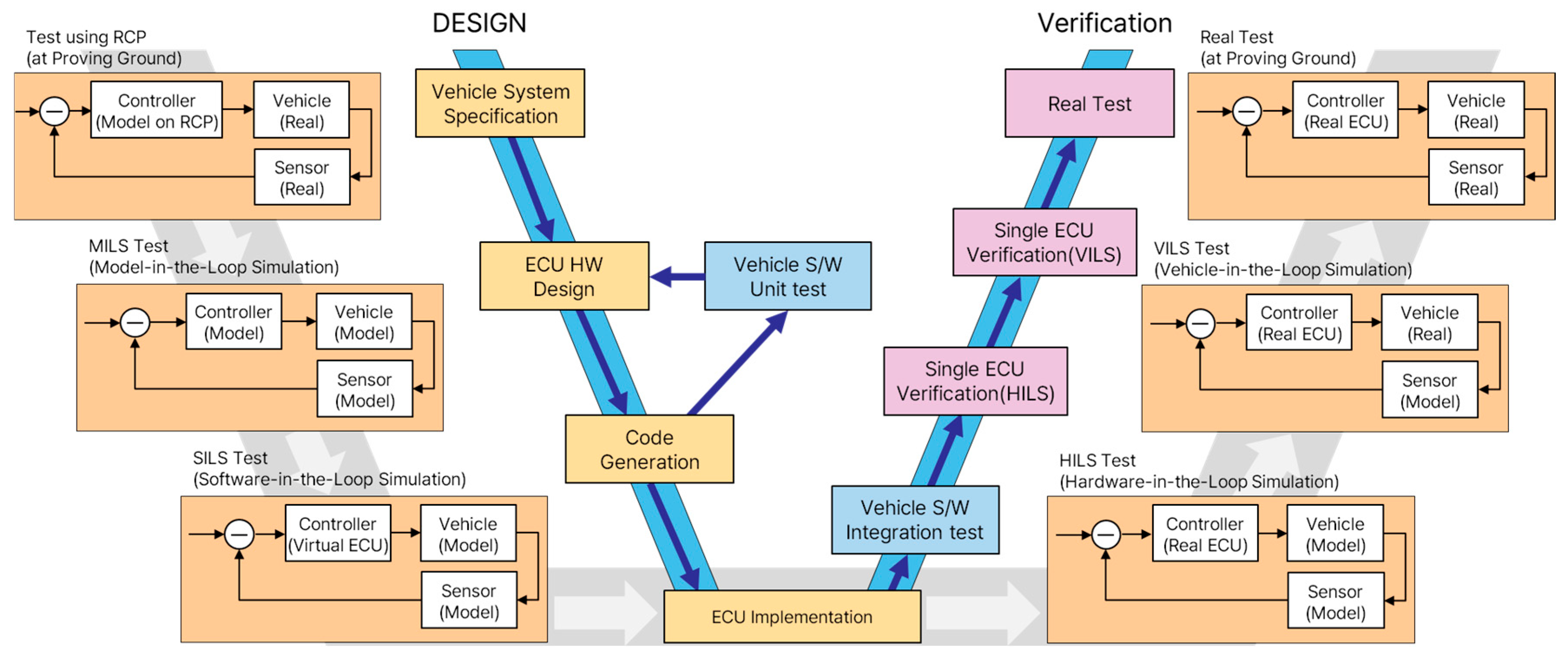
XILS-based techniques have been actively researched and utilized as a systematic approach to verifying ADS safety. As shown in Figure 1, a key component in the development and validation of ADSs, XILS is categorized into MILS, SILS, HILS, and VILS based on the development stage and constitutes the final step before real-world validation [22]. Figure 1 illustrates the hierarchical integration of XILS technologies within the V-Model development framework. The figure demonstrates systematic progression from early-stage MILS for algorithm verification, through SILS for software validation, HILS for real-time hardware integration testing, to VILS for comprehensive vehicle-level validation, culminating in real vehicle testing. With the continued progress in simulation research, though, the characteristics and limitations of each XILS phase are becoming clearer. Specifically, MILS enables rapid verification of control algorithms and vehicle models within a purely software environment, thus being an effective tool for securing algorithm stability during the initial development phase [23]. However, it is limited by its inability to reflect real hardware characteristics. SILS leverages virtual electronic control unit (ECU) models to systematically validate control software functionality and evaluate software code performance before hardware integration [24]. However, aspects such as actual hardware data structures and computational delays are difficult to emulate perfectly. HILS incorporates real ECUs and hardware for real-time validation and a comprehensive assessment of hardware–software interactions, but it fails to reproduce the complexity of real vehicle dynamics [25,26,27]. To overcome these stage-specific limitations, recent research has focused on VILS, an advanced approach that integrates a real vehicle with a virtual environment, maintaining the vehicle’s dynamic characteristics while enabling safe testing across various virtual scenarios [28].

To address the limitations of existing XILS approaches while maintaining vehicle dynamic fidelity, Son et al. [29] proposed a proving ground (PG)-based VILS system that recreates a real proving ground as a high-definition (HD) map-based virtual road. The system comprises four key components: virtual road generation, real-to-virtual synchronization, virtual traffic behavior generation, and perception sensor modeling. This design preserves the vehicle’s true dynamic characteristics while enabling safe, repeatable testing of various scenarios in a virtual environment. Unlike dynamometer-based VILS, it can be implemented with only a proving ground and does not require large-scale dynamometers or over-the-air (OTA) equipment, which significantly reduces initial infrastructure costs and operational risks. Additionally, by utilizing a virtual road derived from an actual test site, it enhances the reproducibility of experiments. Given these advantages, we adopted the PG-based VILS platform for our XILS case study. Simulation platforms for the evaluation and verification of ADSs have been continuously developed and refined. However, before assessing the consistency of results between real-world experiments and simulations, the credibility of the simulation platform itself must be confirmed.

Oh [30,31] proposed a methodology to implement the AD-VILS platform designed for evaluating ADSs and developed a technique to assess the platform’s reliability based on key test parameters relevant to ADSs. They quantitatively evaluated consistency by comparing these key parameters between real-vehicle tests and VILS tests based on statistical indicators. Furthermore, they proposed a scenario-based reliability evaluation method to verify whether VILS testing could partially replace real-world testing or be effective in specific scenarios. Based on the indices of consistency between real-vehicle tests and VILS tests, they derived correlation and applicability metrics to evaluate the platform’s overall reliability. However, existing credibility-assessment techniques for XILS platforms still have significant limitations. Major issues include their focus on evaluating advanced driver assistance system (ADAS) functions without sufficiently considering the overall dynamic behavior of the vehicle. Furthermore, most verification frameworks are limited to low-speed scenarios, which hinders reliability verification under higher-speed conditions. Additionally, the requirement for repeating independent experiments under different speed conditions represents a significant structural inefficiency.

Therefore, we propose a novel framework for evaluating the credibility of XILS platforms as a virtual tool chain for ADS validation. The strategy involves statistical and mathematical comparisons between the results of XILS tests and real-vehicle tests, with similarity and consistency metrics calculated for each test. These metrics are determined from the perspectives of parameters, scenarios, and dynamics, and the calculated consistency enables evaluation across three aspects: parameter-based reliability, scenario-based reliability, and dynamics-based fidelity. Ultimately, the credibility of the XILS platform is determined based on the results of these three types of analyses. Furthermore, to ensure efficient credibility evaluation, geometric similarity analysis is performed. The credibility evaluation metrics, derived from experimental data obtained through tests conducted under various speed conditions within the same scenario, are visualized on spider charts. The use of geometric shape comparison metrics allows quantitative analysis of the similarity between two shapes, demonstrating that speed is not the dominant factor when assessing scenario credibility. Additionally, the analysis of geometric similarities between different scenarios suggests the possibility of establishing a representativeness assessment framework, where certain scenarios can serve as proxies for the credibility assessment of others.

The systematic credibility evaluation framework proposed herein is expected to efficiently verify whether virtual XILS test results remain valid in real-world driving environments, thereby serving as a dependable foundation for the development of ADSs.

The remainder of this paper is structured as follows: Section 3 explains the proposed credibility-assessment methodology, which is based on an integrated evaluation framework that considers not only reliability but also fidelity while reflecting dynamic consistency. Section 4 introduces the procedures for efficiently verifying the credibility of XILS platforms, which is followed by a test to determine whether the speed condition is the dominant factor when assessing a given scenario. The credibility-assessment results across various speed conditions within the same scenario are visualized through spider charts, and the similarity between shapes is quantitatively analyzed through geometric shape comparison. This similarity analysis serves as the basis for evaluating the efficiency of credibility validation. Furthermore, we extend the geometric shape comparison to scenarios involving different driving maneuvers to establish a methodology for confirming whether certain scenarios can represent others. Section 5 describes the experimental environment created for the real-vehicle tests and VILS tests and discusses the validity of the methods outlined in Section 3 and Section 4 based on experimental results. Finally, Section 6 presents the implications of our findings for the credibility assessment of simulation platforms, states the limitations of this study, and outlines future research directions.

3. Proposed Credibility Evaluation Methodology

Before utilizing XILS environments for ADS validation, the credibility of the XILS platform itself must be rigorously assessed.

It is important to clarify the distinction between credibility, reliability, and fidelity as used in this framework. Following UNECE DCAS regulations, credibility represents a comprehensive assessment that encompasses both reliability (the consistency and repeatability of results under identical conditions) and fidelity (the accuracy with which simulation models reproduce real-world physical characteristics and behaviors). While reliability focuses on reproducibility and consistency between repeated tests, fidelity emphasizes the physical accuracy of dynamic responses. Credibility, therefore, serves as an overarching metric that ensures a simulation platform is both consistent in its outputs and accurate in its representation of real-world phenomena, making it fit for its intended validation purpose.

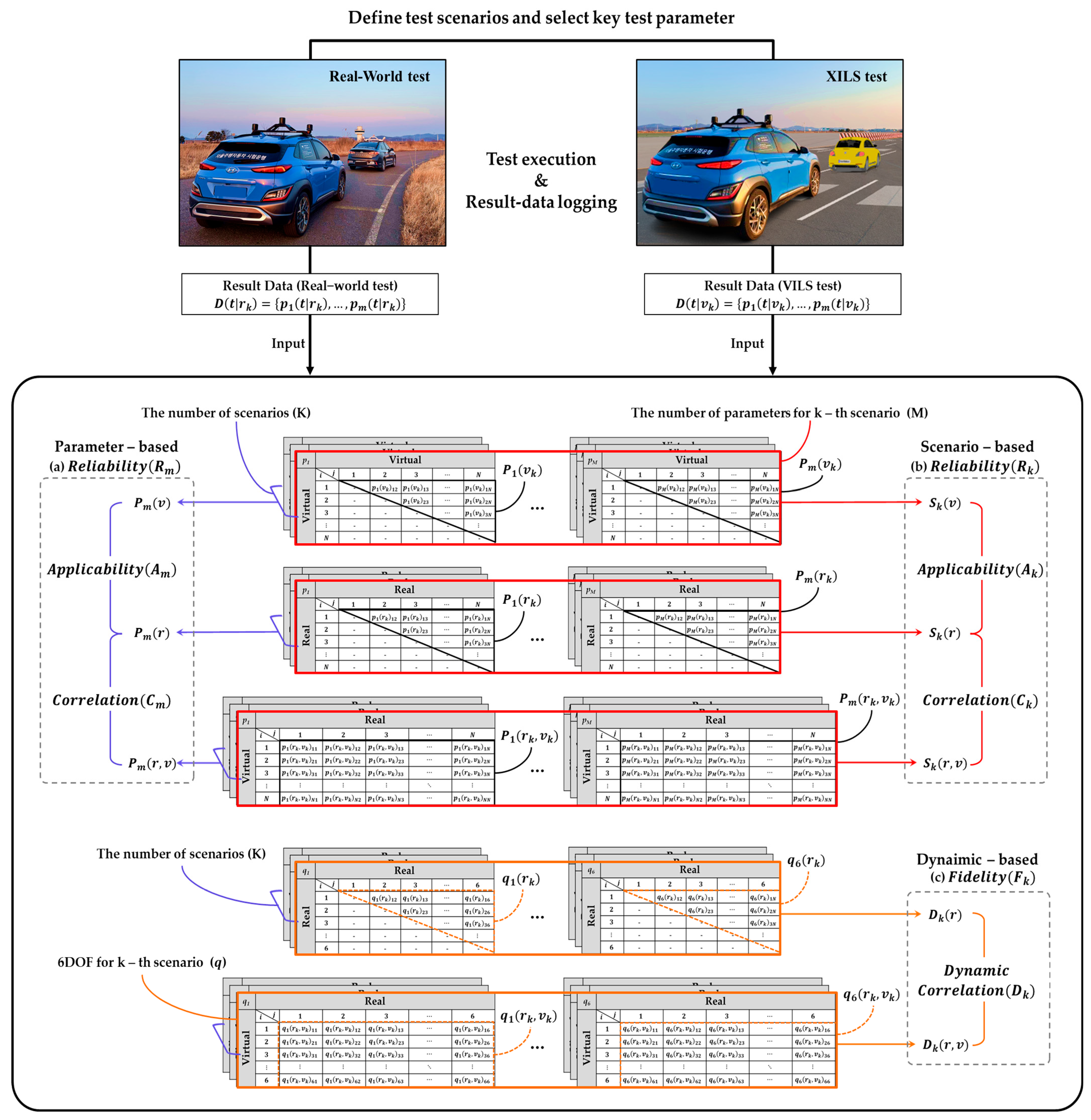
We propose a framework to quantify the credibility of XILS through a comprehensive assessment from parameter-based, scenario-based, and dynamics-based perspectives (Figure 2).

Figure 2 presents the comprehensive three-dimensional credibility evaluation framework for XILS platforms, building upon the reliability assessment methodology established by Oh [31]. The framework illustrates a systematic matrix-based comparison structure that processes similarity calculations between different test configurations (virtual–virtual, real–real, and virtual–real combinations) across multiple dimensions. The core of the methodology centers on structured similarity matrices where each table represents different comparison types indicated by the (virtual, real) labels at the top and left sides. Within each matrix, black-bordered cells represent the similarity comparison results for individual parameters (one of m parameters) between specific test iterations, enabling detailed component-level analysis. Red-bordered horizontal sections encompass the similarity results for all m parameters within a single scenario (one of k scenarios), providing scenario-level aggregated comparisons. Blue-bordered vertical stacks represent similarity results for a single parameter (one of m parameters) across all k scenarios, facilitating parameter-level cross-scenario analysis. These multi-layered matrix structures feed into the three parallel evaluation streams: (1) Parameter-based reliability assessment utilizes the blue-bordered parameter stacks to calculate correlation indices $\left(C_m\right)$ and applicability indices $\left(A_m\right)$ for each of the m key parameters, identifying specific modeling deficiencies in simulation components; (2) scenario-based reliability assessment leverages the red-bordered scenario sections to compute scenario-level correlation $\left(C_k\right)$ and applicability $\left(A_k\right)$ indices, determining replacement feasibility of real-world tests; (3) dynamics-based fidelity assessment employs additional orange-bordered matrices that specifically compare six-degree-of-freedom motion characteristics between virtual and real test configurations, yielding dynamic correlation indices $\left(D_k\right)$. Validation test scenarios and key test parameters are defined, and data are then collected by performing repeated real-world and XILS tests under identical conditions. The collected data are analyzed across three core dimensions before being integrated into the final credibility assessment.

The parameter-based reliability assessment involves calculating the applicability index ($A_m$) and correlation index ($C_m$) for each key test parameter. The applicability index determines whether XILS tests offer better repeatability and reproducibility than real-world tests, quantifying the consistency of individual component models within the XILS platform in maintaining their outputs across multiple test iterations. The correlation index measures the similarity between real-world and XILS tests at the parameter level, reflecting the accuracy of the simulation component models with reference to the respective parameters. The parameter-based reliability ($R_m$) is then evaluated based on whether these two indices meet their defined evaluation criteria.

Scenario-based reliability assessment involves calculating the applicability index ($A_k$) and correlation index ($C_k$) for each scenario. The scenario applicability index quantifies how consistently XILS test results align with real-world test results in a given scenario, while the scenario correlation index measures the overall similarity between real-world and XILS tests at the scenario level. The scenario-based reliability ($R_k$) is then determined based on whether these two indices meet their predefined evaluation criteria.

Dynamics-based fidelity assessment involves calculating the dynamic correlation index ($D_k$) centered on the vehicle’s six-degree-of-freedom (6DOF) motion characteristics. This index measures the similarity between real-world tests and XILS tests based on information on the vehicle’s three types of translational movements and three types of rotational movements. The dynamics-based fidelity ($F_k$) is then evaluated based on whether $D_k$ meets the defined evaluation criterion.

When the parameter-based reliability ($R_m$), scenario-based reliability ($R_k$), and dynamics-based fidelity ($F_k$) have all been validly assessed, the XILS platform is deemed credible. This multi-dimensional approach minimizes the potential biases arising from single-perspective evaluations and comprehensively verifies the credibility of the XILS platform for ADS validation.

We employed the comparative analysis techniques proposed by Oh [31] to measure the similarity between the datasets from the real-world and XILS tests. Oh [31] proposed a comprehensive similarity evaluation metric that combines the correlation coefficient ($f_1$) for integrated comparison, the Zilliacus error ($f_2$) for point-to-point comparison, and the Geers metric ($f_3$) to analyze magnitude and phase errors separately.

The correlation coefficient $\left(f_1\right)$ is defined by Equation (1), where $y_1$ and $y_2$ represent the two datasets to be compared, and $\omega$ denotes the number of sample data points, with each data point indexed by $i$ from 0 to $\omega$ [32]. The correlation coefficient ranges from −1 to 1, where values closer to 1 indicate stronger positive linear relationships between the dataset trends. The Zilliacus error $\left(f_2\right)$ is calculated using Equation (2), which normalizes the sum of absolute point-wise errors $\left|y_{1,i}-y_{2,i}\right|$ by the sum of absolute values of the reference dataset; lower f₂ values indicate better point-to-point agreement between the two datasets [33]. The Geers metric $\left(f_3\right)$ is calculated as the square root of the sum of the squares of the magnitude error $\left(M_G\right)$ and phase error $\left(P_G\right)$, as expressed in Equation (3). The magnitude error $M_G$ in Equation (4) quantifies the energy ratio between datasets through their squared sums, while the phase error $P_G$ in Equation (5) measures temporal alignment differences using normalized cross-correlation [34]. This technique enables separate evaluations of amplitude differences and temporal synchronization between the datasets.

Finally, the combined similarity metric ($y_R$) is calculated as the weighted sum of these three indicators, as shown in Equation (6). Here, ${\mathsf{\eta }}_1, {\mathsf{\eta }}_2$, and ${\mathsf{\eta }}_3$ represent the weighting factors for the three metrics, which can be adjusted according to their respective importance levels. In this study, equal weighting $\left({\eta }_1={\eta }_2={\eta }_3=1/3\right)$ was applied to ensure balanced consideration of all three similarity aspects. However, these weights can be adjusted according to specific testing requirements and the relative importance of each metric for different evaluation contexts. Since the complete mathematical derivation and information regarding each metric have already been provided by Oh [31], in-depth discussion is omitted in this paper.

$$f_1={\displaystyle \frac{\omega {\sum }_{i=0}^{\omega }{y}_{1,i}{y}_{2,i}-{\sum }_{i=0}^{\omega }{y}_{1,i}{\sum }_{i=0}^{\omega }{y}_{2,i}}{\sqrt{\omega {\sum }_{i=0}^{\omega }{y}_{1,i}^2-{\left({\sum }_{i=0}^{\omega }{y}_{1,i}\right)}^2}\cdot \sqrt{\omega {\sum }_{i=0}^{\omega }{y}_{2,i}^2-{\left({\sum }_{i=0}^{\omega }{y}_{2,i}\right)}^2}}},$$

(1)

$$f_2={\displaystyle \frac{{\sum }_{i=0}^{\omega }\left|y_{1,i}-y_{2,i}\right|}{{\sum }_{i=0}^{\omega }\left|y_{2,i}\right|}},$$

(2)

$$f_3=\sqrt{M_G^2+P_G^2},$$

(3)

$$M_G=\sqrt{{\displaystyle \frac{{\sum }_{i=0}^{\mathsf{\omega }}{y}_{1,i}^2}{{\sum }_{i=0}^{\mathsf{\omega }}{y}_{2,i}^2}}}-1,$$

(4)

$$P_G=1-{\displaystyle \frac{{\sum }_{i=0}^{\omega }{y}_{1,i}{y}_{2,i}}{\sqrt{{\sum }_{i=0}^{\omega }{y}_{1,i}^2{\sum }_{i=0}^{\omega }{y}_{2,i}^2}}},$$

(5)

$$y_R\left(y_1,y_2\right)={\mathsf{\eta }}_1{f}_1+{\mathsf{\eta }}_2\left(1-f_2\right)+{\mathsf{\eta }}_3\left(1-f_3\right).$$

(6)

We used this integrated similarity index to evaluate the reliability of XILS from a parameter perspective and a scenario perspective, as explained in Section 3.2 and Section 3.3, respectively. The evaluation of the XILS platform’s fidelity from a dynamics perspective is described in Section 3.4.

3.1. Definitions of Scenarios and Parameters

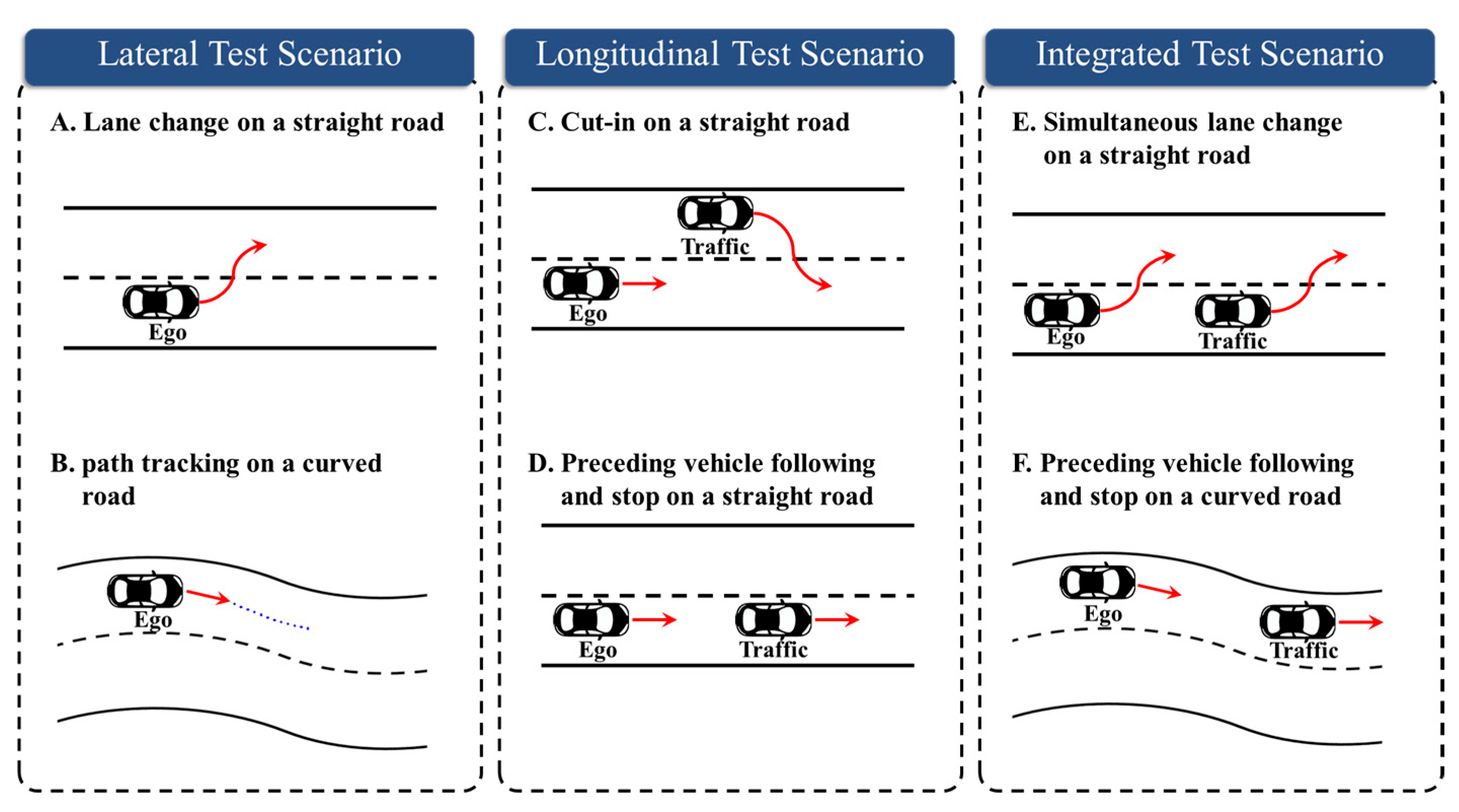
To evaluate the credibility of XILS platforms, the test scenarios and key test parameters must be systematically defined. This section outlines the scenario selection criteria and the key parameters used in the proposed evaluation framework. We constructed six test scenarios based on driving conditions and maneuver types. Based on the control characteristics, these scenarios are categorized into lateral (A and B), longitudinal (C and D), and integrated (E and F) evaluation. Figure 3 illustrates each scenario.

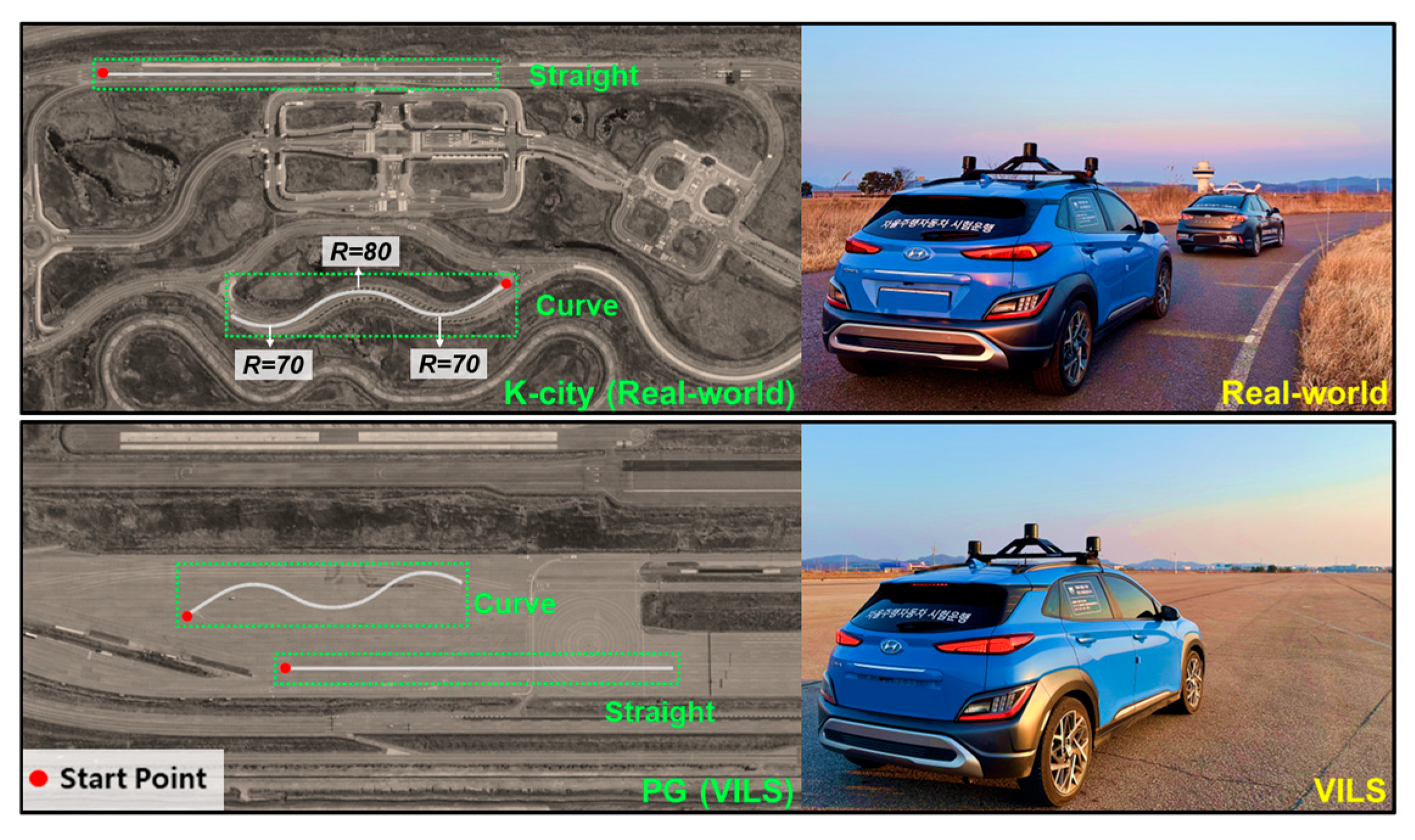
The lateral evaluation scenarios were designed to verify the steering performance and lateral stability of the subject vehicle. Scenario A represents a situation where the subject vehicle changes lanes on a straight road without any external environmental influence, while driving at speeds of 30 km/h, 50 km/h, and 70 km/h. Scenario B evaluates the vehicle’s ability to stably follow a trajectory created based on information provided by the global positioning system (GPS) sensor on an S-shaped road, while driving at speeds of 20 km/h, 40 km/h, and 60 km/h.

The longitudinal evaluation scenarios were intended to verify the subject vehicle’s speed control and its interaction with a target vehicle. Scenario C involves a cut-in maneuver on a straight road, designed to evaluate the effectiveness of the adaptive cruise control function in maintaining a safe distance from the vehicle ahead. Scenario D focuses on testing the subject vehicle’s ability to maintain a constant distance behind a slower target vehicle on a straight road. In both scenarios, the subject vehicle’s speeds are 60 km/h, 80 km/h, and 100 km/h, while the target vehicle’s speeds are 40 km/h, 60 km/h, and 80 km/h.

The integrated evaluation scenarios were designed to analyze complex situations requiring simultaneous lateral and longitudinal control. Scenario E evaluates the subject vehicle’s ability to perform steering and speed control while maintaining a stable distance from the vehicle ahead when both vehicles simultaneously change lanes on a straight road. In this scenario, the subject vehicle’s speeds are set at 60 km/h, 80 km/h, and 100 km/h, while the target vehicle’s speeds are set at 40 km/h, 50 km/h, and 80 km/h. Scenario F comprehensively assesses the subject vehicle’s lateral stability and longitudinal following control while it drives behind the target vehicle on a curved road. In this scenario, the subject vehicle’s speeds are 40 km/h, 60 km/h, and 80 km/h, while the target vehicle’s speeds are 30 km/h, 40 km/h, and 50 km/h.

In all six scenarios, the target vehicle utilizes a speed control method to maintain the specified target speeds; however, it may or may not reach the target speeds depending on the situation. By conducting experiments under these diverse scenarios, the performance of the ADS and the credibility of the XILS platform can be comprehensively evaluated.

Table 1. Classification of key test parameters based on maneuver (scenario) types.

Signal		Frame	Unit	Maneuver (Scenario)
$\mathrm{Lateral} \mathrm{acceleration} \left(a_y\right)$		Vehicle	${\displaystyle \raisebox{1ex}{$\mathrm{m}$}\!\left/ \!\raisebox{-1ex}{${\mathrm{s}}^2$}\right.}$	Lateral (A, B)	Integrated (E, F)
$\mathrm{Yaw} \mathrm{rate} \left(\gamma \right)$		Vehicle	${\displaystyle \raisebox{1ex}{$\mathrm{d}\mathrm{e}\mathrm{g}$}\!\left/ \!\raisebox{-1ex}{$\mathrm{s}$}\right.}$
$\mathrm{Desired} \mathrm{steering} \mathrm{wheel} \mathrm{angle} \left({\delta }_{des}\right)$		Vehicle	$°$
$\mathrm{Longitudinal} \mathrm{position} \left(X\right)$		Global	$\mathrm{m}$
$\mathrm{Lateral} \mathrm{position} \left(Y\right)$		Global	$\mathrm{m}$
$\mathrm{Yaw} \mathrm{angle} \left(\psi \right)$		Global	$°$
$\mathrm{Longitudinal} \mathrm{acceleration} \left(a_x\right)$		Vehicle	${\displaystyle \raisebox{1ex}{$\mathrm{m}$}\!\left/ \!\raisebox{-1ex}{${\mathrm{s}}^2$}\right.}$	Longitudinal (C, D)
$\mathrm{Velocity} \left(V_e\right)$		Vehicle	${\displaystyle \raisebox{1ex}{$\mathrm{m}$}\!\left/ \!\raisebox{-1ex}{$\mathrm{s}$}\right.}$
$\mathrm{Desired} \mathrm{longitudinal} \mathrm{acceleration} \left(a_{x,des}\right)$		Vehicle	${\displaystyle \raisebox{1ex}{$\mathrm{m}$}\!\left/ \!\raisebox{-1ex}{${\mathrm{s}}^2$}\right.}$
Object state	$\mathrm{Relative} \mathrm{longitudinal} \mathrm{distance} \left({RD}_x\right)$	Vehicle	$\mathrm{m}$
	$\mathrm{Relative} \mathrm{lateral} \mathrm{distance} \left({RD}_y\right)$	Vehicle	$\mathrm{m}$
	$\mathrm{Relative} \mathrm{velocity} \left(RV\right)$	Vehicle	${\displaystyle \raisebox{1ex}{$\mathrm{m}$}\!\left/ \!\raisebox{-1ex}{$\mathrm{s}$}\right.}$

lists the main test parameters used in this study, which are defined as internal signals reflecting the core operations of the ADS and consist of vehicle status information, object data based on perception sensors, and control commands.

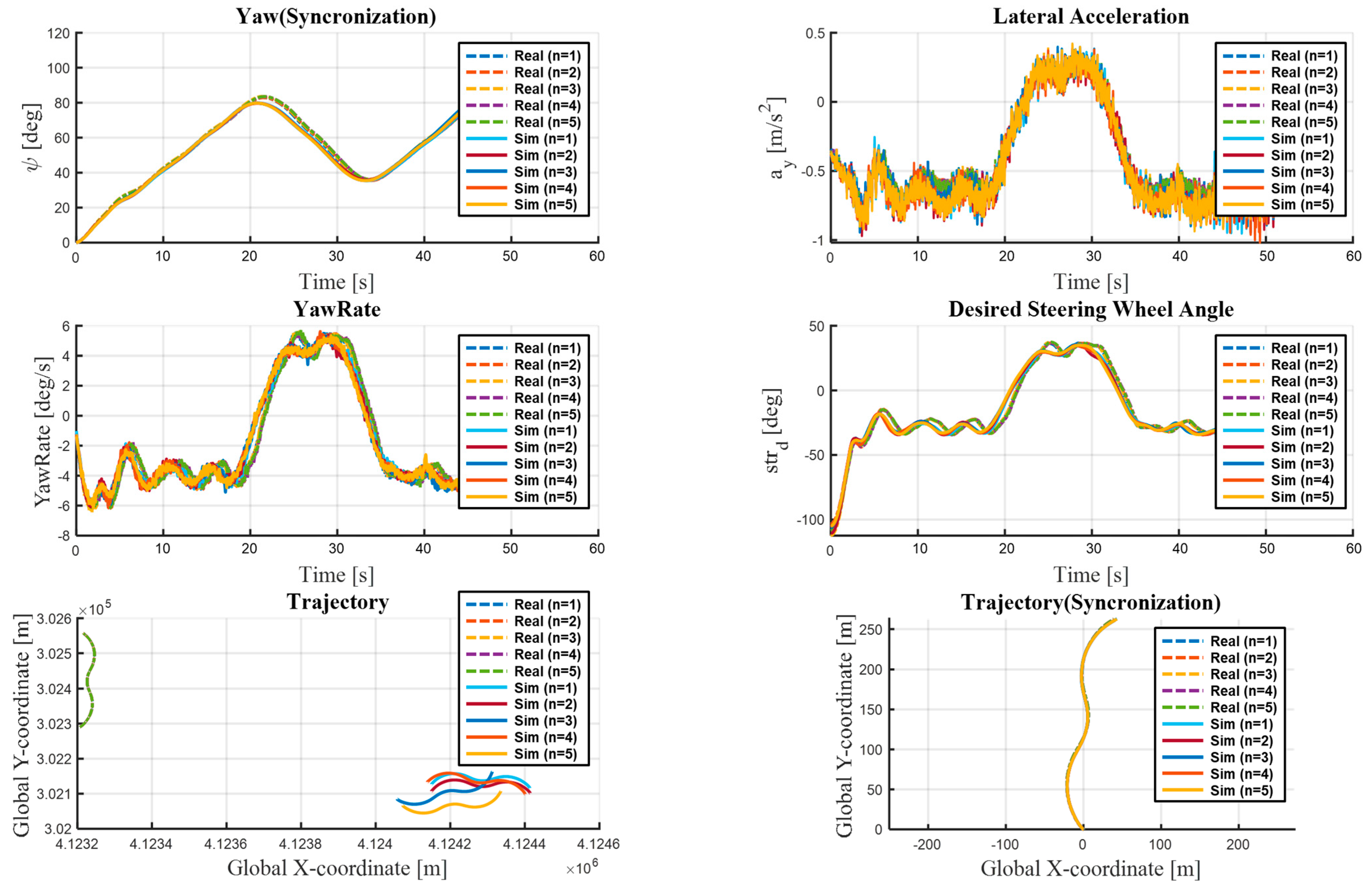
For the lateral evaluation scenarios (A and B), lateral acceleration ($a_y$), yaw rate ($\gamma$), and target steering angle (${\delta }_{des}$) were selected as the primary metrics. These parameters are instrumental for a precise quantitative assessment of lateral control performance during lane-change maneuvers and curved-road navigation.

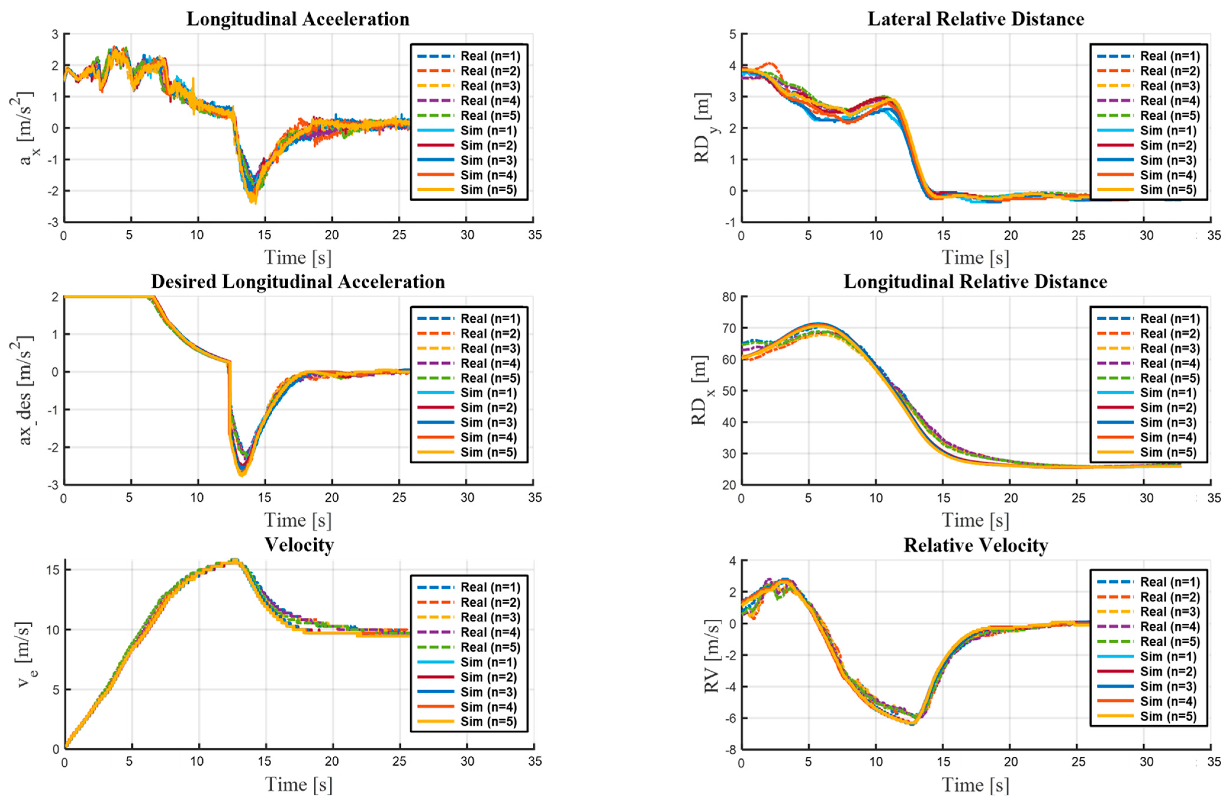
For the longitudinal evaluation scenarios (C and D), we employed longitudinal acceleration ($a_x$), vehicle speed ($V_e$), target longitudinal acceleration ($a_{x,des}$), relative longitudinal distance ($R{D}_x$), relative lateral distance ($R{D}_y$), and relative speed (RV) as the core evaluation metrics. These measures are paramount for robust evaluation of whether a safe following distance is maintained and if speed is suitably regulated relative to a lead vehicle.

In the integrated assessment scenarios (E and F), the lateral and longitudinal metrics were combined to ensure a holistic assessment framework for analyzing system performance under complex maneuvering conditions.

The simulations in this study were performed in a VILS environment built using IPG CarMaker HIL 10.2, a high-fidelity autonomous driving and vehicle dynamics simulation software program. A realistic test environment was implemented using a high-fidelity vehicle dynamics model and an object list-based perception sensor model. Specifically, we focused on evaluating the accuracy of the relative distance and relative velocity to analyze the effects of sensor noise and uncertainty on the performance of the ADS [35,36,37]. This approach contributed to improving the similarity between simulated and actual driving and enhancing the credibility of the evaluation results.

3.2. Parameter-Based Reliability Evaluation

We adopted the parameter-based reliability evaluation method proposed by Oh [31], which enables the accuracy of the simulation component models used in XILS to be verified indirectly. For each scenario, we conducted N identical trials of both the XILS test and the real-vehicle test and compared the obtained parameter values to calculate three types of consistency indices: intra-XILS consistency ($P_m\left(v\right)$), intra-real-vehicle consistency ($P_m\left(r\right)$), and XILS–real-vehicle consistency ($P_m\left(v,r\right)$). Based on these indices, the correlation index $C_m$ and the application index $A_m$ are calculated as shown in Equations (7) and (8), respectively, as follows:

$$C_m={\displaystyle \frac{P_m\left(v,r\right)}{P_m\left(r\right)}}\times 100\hspace{0.17em}\left(\%\right),$$

(7)

$$A_m={\displaystyle \frac{P_m\left(v\right)}{P_m\left(r\right)}}\times 100\hspace{0.17em}\left(\%\right).$$

(8)

The correlation index $C_m$ represents the similarity between the results of the XILS tests and the real-vehicle tests, with values close to 100% indicating highly accurate simulation models. The applicability index $A_m$ exceeding 100% means that the repeatability and reproducibility of the XILS test are better than those of the real-vehicle test. The XILS platform is considered to achieve parameter-based reliability $R_m$ when all criteria in Equation (9) are met:

$$R_m=\left(C_m>{\alpha }_P\right)\cap \left(A_m>{\beta }_P\right),\hspace{1em}m\in \{\mathrm{1,2},\dots ,M\}$$

(9)

where ${\mathsf{\alpha }}_P$ and ${\mathsf{\beta }}_P$ denote the correlation evaluation criterion and the applicability evaluation criterion, which are defined in Equations (10) and (11), respectively:

$${\alpha }_P=C_P-{\sigma }_P,$$

(10)

$${\beta }_P=Q-{\sigma }_P,\hspace{1em}\left(Q=1\right)$$

(11)

where $C_P$ denotes the minimum value among the maximum consistency indices for the real-vehicle tests, and ${\mathsf{\sigma }}_P$ is the average deviation between the maximum and minimum consistency indices of these tests. These criteria imply that the normalized consistency of the XILS trials must exceed that of the real-vehicle trials to guarantee superior repeatability and reproducibility.

The evaluation criteria ${\alpha }_P$ and ${\beta }_P$ are established based on empirical data analysis to ensure statistical robustness. As detailed in Oh ([31], Equations (19)–(24)), ${\alpha }_P$ is derived from the principle that XILS-to-real-world consistency must exceed the normalized consistency observed within real-world tests alone, with ${\sigma }_P$ accounting for inherent experimental variability. The criterion ${\beta }_P$ assumes ideal simulation repeatability $\left(Q=1\right)$ while incorporating the same variability measure, ensuring XILS demonstrates superior reproducibility compared to real-world testing conditions.

This method enables prior identification of any specific parameters that could undermine the XILS platform’s reliability, whereby the accuracy of the corresponding simulation models can be refined accordingly. As the complete derivation of the parameter-based evaluation equation is provided by Oh [31], it is omitted herein.

3.3. Scenario-Based Reliability Evaluation

We employed the scenario-based reliability assessment method proposed by Oh [31], the primary objective of which is to assess whether XILS tests can effectively replace real-vehicle tests in a given scenario. For each scenario, we conducted N trials of both the XILS and real-vehicle tests to calculate three types of scenario consistency indices: intra-XILS consistency ($S_k\left(v\right)$), intra-real-vehicle consistency ($S_k\left(r\right)$), and XILS–real-vehicle consistency ($S_k\left(v,r\right)$). Based on these indices, the scenario correlation index $C_k$ and the applicability index $A_k$ are calculated as shown in Equations (12) and (13):

$$C_k={\displaystyle \frac{S_k\left(v,r\right)}{S_k\left(r\right)}}\times 100\hspace{0.17em}\left(\%\right),$$

(12)

$$A_k={\displaystyle \frac{S_k\left(v\right)}{S_k\left(r\right)}}\times 100\hspace{0.17em}\left(\%\right).$$

(13)

A scenario correlation index $C_k$ close to 100% indicates a very high similarity between the XILS and real-vehicle test results in that scenario, while an applicability index $A_k$ exceeding 100% indicates that the repeatability and reproducibility of the XILS tests are better than those of the real-vehicle tests. The XILS platform is deemed to attain scenario-based reliability $R_k$ when all the criteria in Equation (14) are met:

$$R_k=\left(C_k>{\alpha }_S\right)\cap \left(A_k>{\beta }_S\right),\hspace{1em}k\in \{\mathrm{1,2},\dots ,K\},$$

(14)

where ${\mathsf{\alpha }}_S$ and ${\mathsf{\beta }}_S$ denote the correlation evaluation criterion and the applicability evaluation criterion, which are defined in Equations (15) and (16), respectively:

$${\alpha }_S=C_S-{\sigma }_S,$$

(15)

$${\mathsf{\beta }}_S=Q-{\mathsf{\sigma }}_S,\hspace{1em}\left(Q=1\right),$$

(16)

where $C_S$ denotes the minimum value among the maximum scenario consistency indices for the real-vehicle tests, and ${\mathsf{\sigma }}_S$ is the average deviation between the maximum and minimum consistency indices across these tests. These criteria imply that the normalized consistency of the XILS trials must exceed that of the real-vehicle trials to guarantee superior repeatability and reproducibility.

The scenario evaluation-based thresholds ${\alpha }_S$ and ${\beta }_S$ follow the same statistical framework as parameter-based criteria but are applied at the scenario evaluation. Following the methodology detailed in Oh ([31], Equations (34)–(39)), these thresholds are derived from the distribution of consistency indices across all test scenarios, ensuring that evaluation criteria reflect realistic performance expectations while maintaining statistical validity for scenario-specific assessments.

This method allows for pre-assessing whether XILS can effectively replace real-vehicle testing in a given scenario, thereby enhancing the efficiency of simulation-based validation. The complete derivation of the scenario-based evaluation equation is excluded from this paper as it has been provided by Oh [31].

3.4. Dynamics-Based Fidelity Evaluation

While the parameter-based and scenario-based evaluations discussed earlier are useful for quantifying the consistency between real-vehicle tests and XILS tests, they cannot fully capture the complex physical phenomena that a vehicle experiences during actual driving. For example, the vertical behavior of a vehicle when driving on irregular surfaces, the interaction between translational and rotational motions due to crosswinds, and the nonlinear lateral dynamics that occur during sudden steering cannot be fully assessed through simple input–output comparisons [38,39,40]. If these vehicle dynamics characteristics under real disturbance conditions are not properly reflected in the simulation model, applying results obtained from the virtual environment to real-world situations can lead to unpredictable errors and compromise safety [41,42,43]. Therefore, we propose a dynamics-based evaluation method to assess how faithfully the simulation reproduces the physical dynamics of the vehicle. Simulations using 3DOF models have been performed to quantitatively analyze the longitudinal and lateral behavior of vehicles, and various control strategies and driving stability techniques have been developed accordingly [44,45]. However, as these models do not fully incorporate the roll, pitch, and yaw variations of the vehicle, they cannot accurately reproduce the dynamic responses observed in real vehicles during high-speed driving, during sudden steering, or under complex road and weather conditions [46,47]. Moreover, with the focus of previous research being on system verification, the physical credibility of simulation platforms themselves has yet to be appropriately assessed.

To overcome these limitations, we introduce a 6DOF model that can precisely evaluate the accuracy of the simulation platform in reproducing the complex dynamic responses of the vehicle body. This method enables objective comparison of the dynamic consistency between the results of simulations and actual tests under various disturbance conditions. The proposed 6DOF model accounts for the vehicle’s longitudinal ($X$), lateral ($Y$), and vertical ($Z$) translational motions, along with its roll ($\phi$), pitch ($\theta$), and yaw ($\psi$) rotational motions; thus, it can describe the vehicle’s complete dynamics by assuming it to be a rigid body based on Newton–Euler equations [48,49]. However, as Coriolis and gyroscopic effects are minimal for vehicles in contact with the ground, these terms are omitted to simplify the model [50,51]. This exclusion significantly reduces the computational load of the simulation while enabling more intuitive and efficient comparison with actual experimental data.

The 6DOF model-based dynamics evaluation significantly enhances the physical credibility of the simulation platform by considering both translational and rotational motions, which 3DOF models fail to achieve. Thus, this evaluation method provides an essential foundation for verifying the credibility of autonomous driving simulation platforms and improving the adaptability of ADSs to real-world driving environments.

The equation of a vehicle’s translational motion explains the relationship between the forces acting when a vehicle moves in space and the resulting acceleration. Considering $m$ to be the vehicle’s mass and $g$ to be Earth’s gravitational acceleration, the forces acting on the vehicle can be defined based on Newton’s second law ($F=m·a$). Along the vehicle’s X-axis (forward–backward direction) and Y-axis (left–right direction), the force is the product of the respective mass and acceleration values. Along the Z-axis (vertical direction), the influence of gravitational acceleration must be additionally considered. Accordingly, these translational motions can be represented by Equation (17), which mathematically expresses the vehicle’s motion in each direction. Here, $a_x,a_y,$ and $a_z$ represent the vehicle’s acceleration along the X-, Y-, and Z-axes, respectively [52].

$$\begin{gathered} F_x=m\cdot a_x, \\ {F}_y=m\cdot a_y, \\ {F}_z=m\cdot \left(a_z-g\right). \end{gathered}$$

(17)

The equation of a vehicle’s rotational motion explains the relationship between torque (moment) and angular acceleration when the vehicle rotates around each axis. Rotational motion is defined by the relationship $M=I·\alpha$, which corresponds to Newton’s second law. Here, the moment of inertia ($I$) along each axis quantifies an object’s resistance to rotational motion. The rotational motions of a vehicle can be represented by Equation (18), which can be utilized to predict and control the vehicle’s attitude changes. Here, $M_x$, $M_y$, and $M_z$ denote the roll moments generated around the X-, Y-, and Z-axes of the vehicle; $I_x, I_y$, and $I_z$ represent the vehicle’s moments of inertia in the roll, pitch, and yaw directions; and $\ddot{\varphi }$, $\ddot{\theta }$, and $\ddot{\psi }$ represent the corresponding angular accelerations, respectively [53].

$$\begin{gathered} M_x=I_x\cdot \ddot{\varphi }, \\ {M}_y=I_y\cdot \ddot{\theta }, \\ {M}_z=I_z\cdot \ddot{\psi }. \end{gathered}$$

(18)

To quantitatively assess the dynamic consistency between simulation tests and real-vehicle tests, the normalized root-mean-square error (NRMSE) was adopted as the primary evaluation metric. NRMSE expresses the deviation between two datasets in a standardized form, enabling objective comparison between variables of different scales [54]. In this study, the credibility of the simulation model was evaluated by systematically quantifying the differences between the simulation results and experimental data based on NRMSE. This evaluation methodology is defined by Equations (19) and (20):

$$f_4\left(y_1, y_2\right)=\sqrt{{\displaystyle \frac{1}{N}}{\sum }_{i=1}^N{\left(y_{2,i}-y_{1,i}\right)}^2},$$

(19)

$$f_5\left(y_1,y_2\right)={\displaystyle \frac{f_4\left(y_1, y_2\right)}{y_{2,max}-y_{2,min}}}\times 100,$$

(20)

where $y_{1,i}$ and $y_{2,i}$ denote the experimental and simulation data, respectively; $N$ is the total number of data samples; and $y_{2,max}$ and $y_{2,min}$ refer to the maximum and minimum values of the experimental or simulation dataset, respectively. The dynamic consistency index, derived from the test parameters in the 6DOF motion equations, is computed by cross-comparing the $i$-th and $j$-th repetitions of the XILS and real-vehicle tests. When the $k$-th scenario is repeated $N$ times in both the XILS and real tests, the results for the $q$-th DOF in the $i$-th XILS repetition and the $j$-th real-test repetition are denoted by $D_q\left(v_{k\left|i\right.}\right)$ and $D_g\left(r_{k\left|j\right.}\right)$, respectively. Based on the comparison metric $f_5$, the dynamic similarity indices for the three types of comparisons between the $i$-th and $j$-th repetitions can be expressed by Equations (21)–(23):

$$D_q{\left(v_k\right)}_{ij}=f_5\left(D_q\left(v_k\left|i\right.\right),D_q\left(v_k\left|j\right.\right)\right),$$

(21)

$$D_q{\left(r_k\right)}_{ij}=f_5\left(D_q\left(r_k\left|i\right.\right), D_q\left(r_k\left|j\right.\right)\right),$$

(22)

$$D_q{\left(v_k,r_k\right)}_{ij}=f_5\left(D_q\left(v_k\left|i\right.\right),D_q\left(r_k\left|j\right.\right)\right).$$

(23)

Equation (23) constitutes a multi-valued dynamic similarity index considering the cross-comparison between repeated tests. To represent these values as a single value for each scenario, Equations (24)–(26) are utilized:

$$D_{q }\left(v_k\right)={\displaystyle \frac{2}{N\left(N-1\right)}}{\sum }_{i=1}^{N-1}{\sum }_{j=2}^N{D}_q{\left(v_k\right)}_{ij},$$

(24)

$$D_{q }\left(r_k\right)={\displaystyle \frac{2}{N\left(N-1\right)}}{\sum }_{i=1}^{N-1}{\sum }_{j=2}^N{D}_q{\left(r_k\right)}_{ij},$$

(25)

$$D_q\left(v_k,r_k\right)={\displaystyle \frac{1}{N^2}}{\sum }_{i=1}^N{\sum }_{j=1}^N{D}_q{\left(v_k,r_k\right)}_{ij}.$$

(26)

The values computed through the three types of comparisons based on Equation (26) represent the dynamic consistency index of the q-th DOF parameter for the k-th scenario. Next, the dynamic consistency indices for all DOFs are weighted and averaged based on Equations (27)–(29) to allow the three types of dynamic consistency indices for the k-th scenario to be expressed as a single value:

$$D_k\left(r\right)={\sum }_{q=1}^6{\eta }_q{D}_q\left(r_k\right),$$

(27)

$$D_k\left(v\right)={\sum }_{q=1}^6{\eta }_q{D}_q\left(v_k\right),$$

(28)

$$D_k\left(v,r\right)={\sum }_{q=1}^6{\eta }_q{D}_q\left(v_k,r_k\right).$$

(29)

The weighting factors ${\eta }_q$ in Equations (27)–(29) for the dynamic consistency indices were set to equal values (${\eta }_q$ = 1/6 for each DOF) to ensure balanced representation of all six degrees of freedom in the dynamics-based evaluation. These weights can be modified based on the specific vehicle dynamics characteristics being emphasized in the evaluation.

Finally, the dynamic correlation index $D_k$ is defined as the ratio of the dynamic consistency index for the inter-real-vehicle-test comparisons to that for the XILS–real-vehicle comparisons, as expressed in Equation (30):

$$D_k={\displaystyle \frac{D_k\left(v,r\right)}{D_k\left(r\right)}}\times 100\hspace{0.17em}\left(\%\right).$$

(30)

$D_k$ approaches 100% as the consistency between the two tests increases, indicating that the simulation component models associated with the 6DOF parameters are highly accurate. Finally, the dynamics-based fidelity $F_k$ of the XILS platform is determined based on whether $D_k$ satisfies the specified acceptance criteria, as expressed in Equation (31):

$$F_k=D_k>{\alpha }_D\hspace{1em}k\in \{\mathrm{1,2},\dots ,K\},$$

(31)

where ${\mathsf{\alpha }}_D$ denotes the dynamic correlation evaluation criterion for $D_k$. As detailed in Equations (32)–(36), ${\mathsf{\alpha }}_D$ is established on the principle that the dynamic consistency between XILS and real-vehicle tests must be greater than or equal to the dynamic consistency observed between repeated real-vehicle tests.

$$D_{\max }\left(r_k\right)=\max \left(D_q\left(r_k\right)\right),\hspace{1em}q\in \{\mathrm{1,2},\dots ,6\},$$

(32)

$$D_{\min }\left(r_k\right)=\min \left(D_q\left(r_k\right)\right),\hspace{1em}q\in \{\mathrm{1,2},\dots ,6\},$$

(33)

$$C_D=\min \left(D_{\max }\left(r_k\right)\right),\hspace{1em}k\in \{\mathrm{1,2},\dots ,K\},$$

(34)

$${\sigma }_D={\displaystyle \frac{1}{K}}{\sum }_{k=1}^K\left(D_{\max }\left(r_k\right)-D_{\min }\left(r_k\right)\right),$$

(35)

$${\alpha }_D=C_D-{\sigma }_D.$$

(36)

In Equations (32)–(36), $D_{\max }\left(r_k\right)$ and $D_{\min }\left(r_k\right),$ respectively, represent the maximum and minimum values of the dynamic consistency index of the $q$-th DOF parameter in each of the k-th scenarios, $C_D$ refers to the minimum value among all $D_{\mathrm{m}\mathrm{a}\mathrm{x}}\left(r_k\right)$ values across the k-th scenarios, and ${\sigma }_D$ indicates the average of the maximum deviations in the consistency indices of the principal DOF parameters across all k-th scenarios.

The dynamic correlation threshold ${\alpha }_D$ is established using a data-driven approach that considers the natural variability inherent in 6DOF vehicle dynamics. As shown in Equations (32)–(36), this threshold is derived from the statistical distribution of dynamic consistency indices across all degrees of freedom, ensuring that XILS platforms demonstrate a dynamic fidelity that meets or exceeds the baseline consistency observed in repeated real-world tests, thereby guaranteeing adequate capture of complex vehicle physical behavior.

If the parameter-based reliability ($R_m$), scenario-based reliability $\left(R_k\right)$, and dynamics-based fidelity ($f_k$) all satisfy their respective evaluation criteria, the XILS implementation under evaluation is considered a credible simulation platform for validating ADSs.

4. Proposed Geometric Similarity Evaluation Methodology

Simulation-based ADS validation is more time-efficient and cost-effective than real-vehicle testing. However, when calculating the credibility of simulation for multiple speed conditions, especially across numerous scenarios, substantial resources are still consumed. Considering the countless situations in which ADSs must operate, a systematic approach is required to improve validation efficiency.

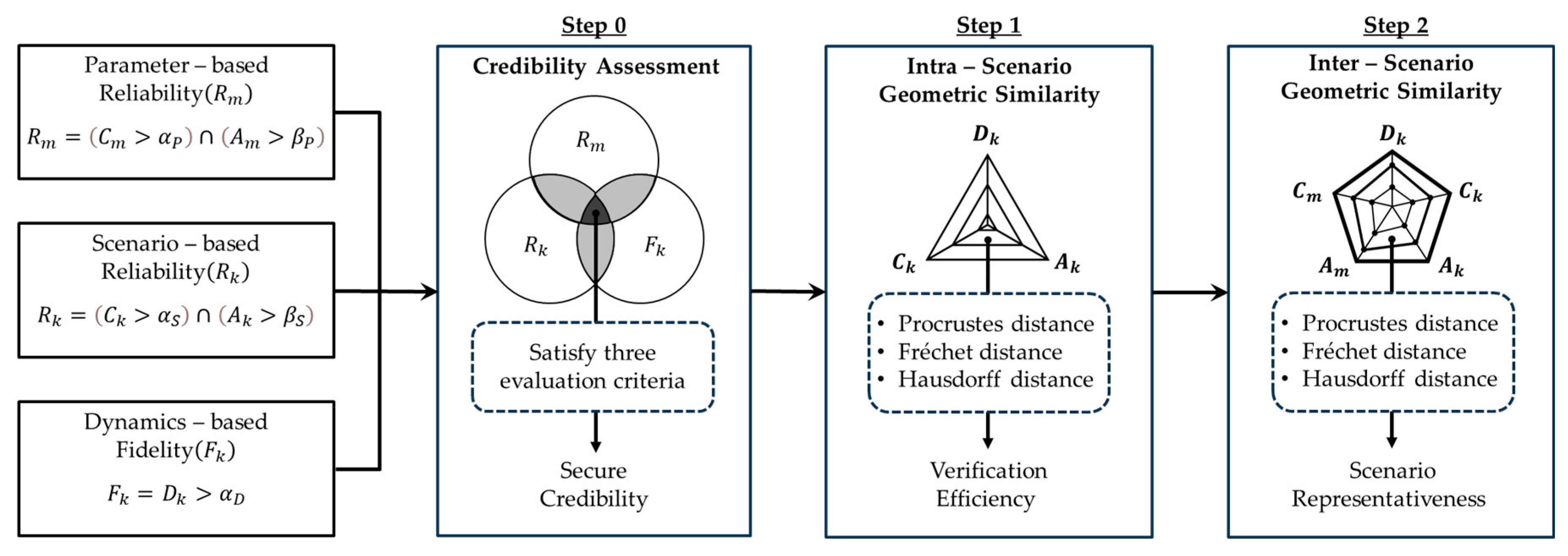
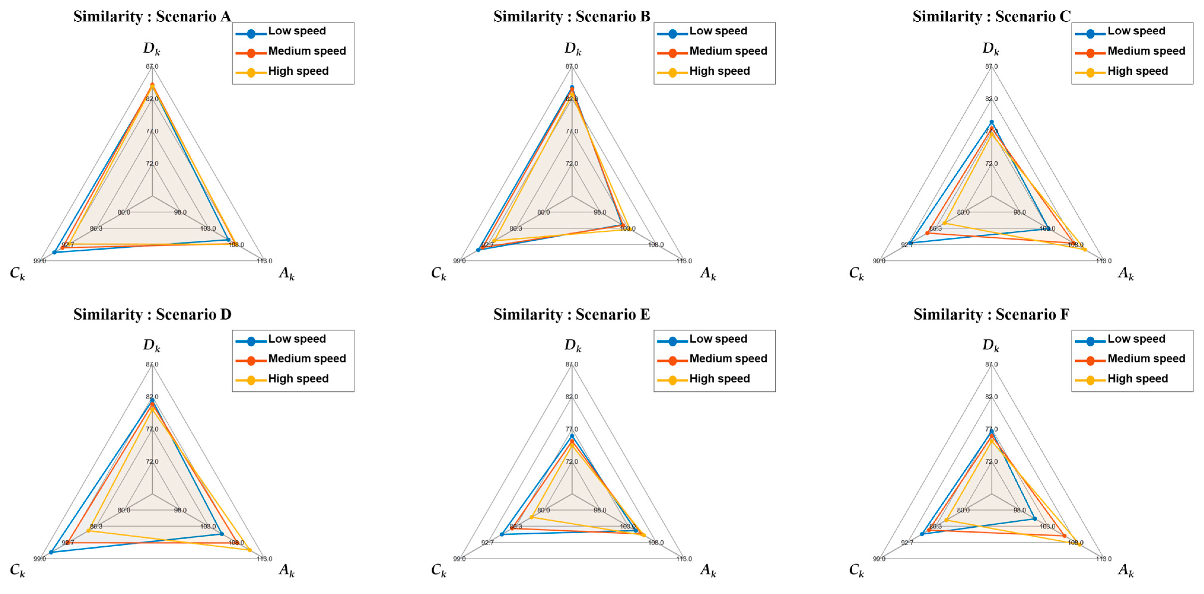
Herein, we propose an efficient credibility verification methodology based on geometric similarity evaluation, as illustrated in Figure 4. In Step 0, three evaluation metrics—parameter-based reliability $\left(R_m\right)$, scenario-based reliability $\left(R_k\right)$, and dynamics-based fidelity $\left(F_k\right)$—are utilized to determine credibility. In Step 1, we evaluate credibility under different speed conditions (low, medium, and high) within the same scenario and visualize the derived evaluation metrics through a spider chart. The geometric similarity between the shapes is analyzed using the Procrustes, Fréchet, and Hausdorff distance techniques. These techniques evaluate the efficiency of the verification process by quantitatively determining whether speed is a dominant factor in the credibility assessment for a given scenario. In Step 2, we additionally evaluate the geometric similarity between different scenarios. This involves verifying whether a particular scenario can represent many other scenarios during credibility assessment.

The proposed assessment framework ensures the credibility of the XILS platforms used to test ADSs while significantly reducing the verification time and cost compared with traditional independent verification approaches. The complete methodology is detailed in Section 4.1 and Section 4.2.

The Procrustes distance quantifies the similarity between two sets of points by optimally aligning them to their common center via rotation, translation, and scaling, before minimizing the sum of the squared errors between the points [55]. This least-squares criterion aligns each configuration’s centroid and allows structural differences to be analyzed via linear transformations, enabling global shape comparison without requiring explicit point-to-point correspondences. Specifically, optimal rotation and scaling solutions are obtained by performing an eigen-decomposition of the transformation matrix between the two configurations.

$$\begin{gathered} f_6=\underset{\lambda ,\mathcal{R},t}{min}{‖y_1-\left(\lambda y_2\mathcal{R}+\mathbf{1}{t}^{\top }\right)‖}_F^2, \\ \mathrm{where} \left\{\mathbf{1}\in {\mathbb{R}}^{\mathrm{n}\times 1}\right\},\mathrm{ }\left\{{\mathrm{t}}^{\mathrm{\top }}\in {\mathbb{R}}^{1\times \mathrm{m}}\right\},\left\{{\mathbf{1}\mathrm{t}}^{\mathrm{\top }}\in {\mathbb{R}}^{\mathrm{n}\times \mathrm{m}}\right\}. \end{gathered}$$

(37)

In Equation (37), the Procrustes distance $f_6$ quantifies similarity based on the global alignment between two point sets $y_1,y_2\in {\mathbb{R}}^{n\times m}$. Here, $n$ denotes the number of points in each shape, $m$ denotes the dimensionality of the space in which each point resides, and each row of the matrix corresponds to a single $m$-dimensional point. Procrustes alignment involves applying the scaling factor $\lambda$, the rotation matrix $\mathcal{R}$, and the translation vector $t$ to $y_2$, in that order, which transforms it into $\lambda y_{2}R+\mathbf{1}{t}^{\top }$. We compute the sum of the squared Frobenius norms of the differences between corresponding points in the transformed point set and $y_1$; subsequently, we define the minimal value of this sum as the Procrustes distance $f_6$. Here, $\mathbf{1}\in {\mathbb{R}}^{\mathrm{n}\times 1}$ is a column vector of ones, and multiplying it by ${\mathrm{t}}^{\mathrm{\top }}\in {\mathbb{R}}^{1\times \mathrm{m}}$ ensures that the same translation vector is applied uniformly to all points. A smaller optimized Frobenius norm indicates that the two point sets are globally well aligned, implying structural similarity.

The Fréchet distance is often illustrated through the analogy of finding the shortest leash length needed to connect a person and a dog as they each walk along their respective curves [56]. This metric captures both the ordering of points along the curves and the overall path flow; hence, it is well suited for comparing time-series data or trajectory-based shapes. Specifically, the discrete Fréchet distance approximation enables efficient computation of this metric in O(pq) time via a dynamic programming-based algorithm.

$$f_7=\underset{\tau \in \mathcal{C}}{min }\underset{(i,j)\in \tau }{max}‖y_{1,i}-y_{2,j}‖.$$

(38)

In Equation (38), $f_7$ is the Fréchet distance, which quantifies the overall path-flow similarity between two point sets $y_1,y_2\in {\mathbb{R}}^{n\times m}$. Each point set is treated as a trajectory of $n$ sequentially connected points, where $y_{1,i}$ and $y_{2,j}$ denote the $i$-th and $j$-th points on the corresponding trajectories, respectively. The correspondence between the two sets is defined by an order-preserving path $\tau =\left(\left(i_1,j_1\right),\left(i_2,j_2\right),\dots \right)$ within the collection $\mathcal{C}$ of such paths. The distances are computed based on the standard Euclidean norm. The Fréchet distance then evaluates the similarity between the trajectories by choosing among all possible paths $\tau$ the one that minimizes the maximum distance between matched points. Hence, a smaller $f_7$ value implies that the two trajectories maintain the same ordering and share similar shapes.

The Hausdorff distance is a metric that measures the distance of every point in Set A from its nearest neighbor in Set B and then finds the maximum value among these nearest-point-pair distances in both directions. Thus, this term quantifies the largest local dissimilarity between two shapes [57]. Because it does not require explicit point-to-point correspondences, it robustly captures shape mismatches even in the presence of small positional errors. Therefore, it is widely used in image comparison and pattern recognition. Additionally, algorithms that approximate the Hausdorff distance on a binary raster grid have been proposed to efficiently compute the minimum over all possible translations.

$$f_8=\mathit{max}\left\{\underset{i\in y_1}{sup}\underset{pj\in y_2}{pinf}‖y_{1,i}-y_{2,j}‖, \underset{i\in y_2}{sup}\underset{pj\in y_1}{pinf}‖y_{2,i}-y_{1,j}‖\right\}.$$

(39)

In Equation (39), $f_8$ represents the Hausdorff distance, which quantifies the maximum local discrepancy between two shapes, i.e., the degree of structural mismatch. The first term reflects the extent to which $y_1$ deviates from $y_2$, while the second term measures the discrepancy in the opposite direction. The maximum of these two values represents the largest bidirectional distance. A smaller $f_8$ indicates that the shapes overlap consistently, whereas a larger value suggests a significant local mismatch (i.e., an outlier). All distances are calculated based on the Euclidean norm.

$$y_S\left(y_1,y_2\right)={\eta }_6{f}_6+{\eta }_7{f}_7+{\eta }_8{f}_8.$$

(40)

As shown in Equation (40), the geometric similarity $\left(y_s\right)$ between two shapes in this study was calculated as a weighted sum of the distance-based metrics from the three perspectives mentioned earlier. This metric was then used to evaluate geometric similarity, as explained in Section 4.1 and Section 4.2

4.1. Geometric Similarity Evaluation

To ensure the credibility of XILS platforms, previous studies have introduced parameter-based and scenario-based evaluation metrics. Herein, we present a new dynamics-based metric. A simulation is deemed credible only when each of these metrics satisfies its predefined evaluation criterion. However, evaluating a single scenario separately under multiple speed conditions increases the number of required tests exponentially, thereby extending both the duration of the process and raising the resource demand. To overcome this challenge, we propose a methodology that quantitatively analyzes the geometric similarity between different speed conditions within the same scenario, which enables the credibility of the platform under untested conditions to be predicted from the results of a single-speed trial. By allowing the overall reliability to be inferred from one experiment, this approach significantly reduces the number of tests needed—and thus the associated time and cost—while also revealing potential compromising factors during the inference process. Hence, this integrated evaluation framework can enhance both the credibility and efficiency of XILS assessments.

Geometric similarity evaluation leverages two scenario-based reliability metrics, namely applicability ($A_k$) and correlation ($C_k$), together with a dynamics-based fidelity metric, namely dynamic correlation ($D_k$). Parameter-based metrics are deliberately excluded from this analysis as they are unsuitable for inter-scenario comparisons and cannot be used to compare different speed conditions within the same scenario. Each metric is rendered as a triangular polygon on a spider chart for each speed condition, which enables a quantitative assessment of geometric similarity across low, medium, and high speeds within a single scenario. By jointly evaluating the structural characteristics of these spider-chart polygons and the interactions among the three metrics, this geometric analysis facilitates a more precise and efficient credibility assessment of XILS platforms. The proposed geometric similarity indices are formulated in Equations (41)–(44):

$$Y_k^L=\left[D_k^L,\hspace{0.25em}{A}_k^L,\hspace{0.25em}{C}_k^L\right],$$

(41)

$$Y_k^M=\left[D_k^M,\hspace{0.25em}{A}_k^M,\hspace{0.25em}{C}_k^M\right],$$

(42)

$$Y_k^H=\left[D_k^H,\hspace{0.25em}{A}_k^H,\hspace{0.25em}{C}_k^H\right],$$

(43)

$$G_k={\displaystyle \frac{1}{3}}\left(y_S\left(Y_k^L,Y_k^M\right)+y_S\left(Y_k^M,Y_k^H\right)+y_S\left(Y_k^L,Y_k^H\right)\right),$$

(44)

where $Y_k^L$, $Y_k^M$, and $Y_k^H$ denote the evaluation-metric vectors for the k-th scenario under low-speed (L), medium-speed (M), and high-speed (H) conditions, respectively. $G_k$ is the geometry-based similarity score for the k-th scenario across its speed conditions, representing the average geometric similarity among the three speed levels; a higher $G_k$ indicates greater structural likeness across speed variations. Finally, as shown in Equation (45), the effectiveness of XILS for the same scenario $E_k$ is evaluated based on whether these similarity scores satisfy a predefined evaluation criterion:

$$E_k=G_k\ge {\alpha }_G\hspace{1em}k\in \{\mathrm{1,2},\dots ,K\},$$

(45)

where ${\alpha }_G$ denotes the geometric similarity evaluation criterion for $G_k$. As expressed in Equations (46)–(50), ${\alpha }_G$ represents the minimum guaranteed level of geometric similarity among the three speed conditions within a given scenario. If $G_k$ equals or exceeds ${\alpha }_G$, the XILS platform’s credibility can be verified based on the results under a single speed condition. The evaluation criterion ${\alpha }_G$, representing the minimum acceptable level of geometric similarity, is derived in a data-driven manner from the distribution of geometric similarity scores across all scenarios. Accordingly, similarity evaluation based on ${\alpha }_G$ relies on the principle that no geometric similarity score may fall below this value.

$$G_{max}\left(k\right)=\max \left({G_k}^{LM},{G_k}^{MH},{G_k}^{HL}\right),\hspace{1em}k\in \{\mathrm{1,2},\dots ,K\},$$

(46)

$$G_{min}\left(k\right)=\min \left({G_k}^{LM},{G_k}^{MH},{G_k}^{HL}\right),\hspace{1em}k\in \{\mathrm{1,2},\dots ,K\},$$

(47)

$$C_G=\min \left(G_{max}\left(k\right)\right),$$

(48)

$${\sigma }_G={\displaystyle \frac{1}{K}}{\sum }_{k=1}^K\left(G_{max}\left(k\right)-G_{min}\left(k\right)\right),$$

(49)

$${\alpha }_G=C_G-{\sigma }_G.$$

(50)

In Equations (46)–(50), $G_{max}\left(k\right)$ and $G_{min}\left(k\right),$ respectively, denote the maximum and minimum geometric similarity indices across the different speed conditions within the same scenario. ${G_k}^{LM},{G_k}^{MH}$, and ${G_k}^{HL}$ denote the geometry-based similarity indices between low and medium speeds, between medium and high speeds, and between high and low speeds, respectively. $C_G$ represents the smallest of the $G_{max}\left(k\right)$ values. In the k-th scenario, ${\sigma }_G$ denotes the average of the maximum deviations in the geometric similarity indices across all scenarios. Thus, we can conclude that for all scenarios where $G_k$ exceeds ${\mathsf{\alpha }}_G$, the geometric similarity between different speed conditions is sufficient, which allows us to assess the credibility of a given scenario without performing individual experiments for different speed levels.

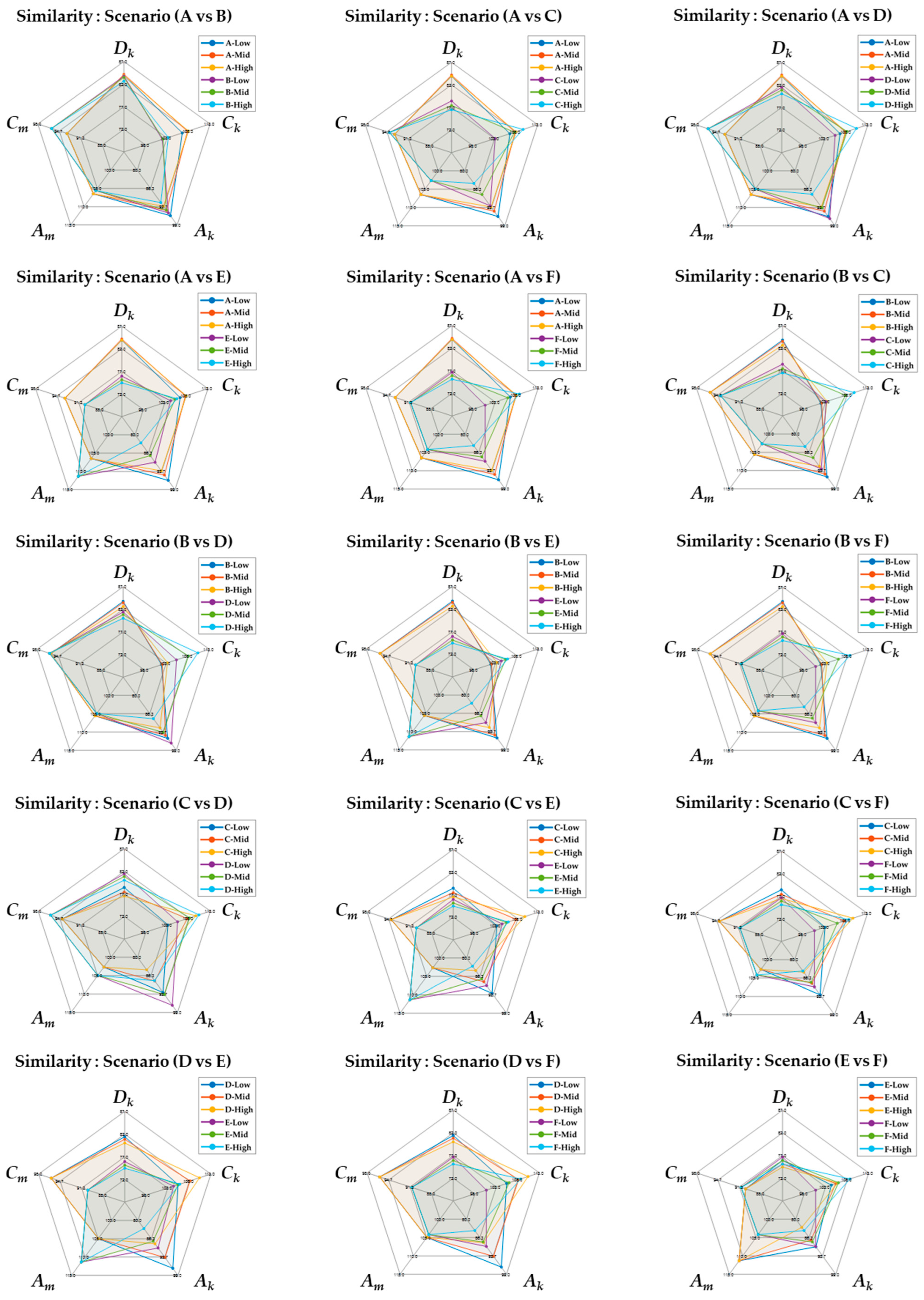
4.2. Scenario Representativeness Evaluation

Building on the process described in Section 4.1, we extended our methodology to assess whether certain entire scenarios can represent other geometrically similar scenarios. Accordingly, based on the premise that the credibility of an XILS platform for different scenarios can be evaluated based on the results from specific representative scenarios for which the platform has already been confirmed to be credible, we propose a scenario representativeness evaluation framework involving geometric similarity calculations between different scenarios.

The evaluation metrics used for the scenario representativeness assessment include parameter-based applicability ($A_m$) and correlation ($C_m$), scenario-based applicability ($A_k$) and correlation ($C_k$), and dynamics-based correlation ($D_k$). The two parameter-based metrics (Am and Cm) are averaged across the different speed conditions (low, medium, and high) within each scenario to obtain a single value that represents the overall parameter applicability and correlation for each scenario. For each k-th scenario, the parameter evaluation scores for each speed condition are calculated as follows: $P_m\left(v_k^L\right)$ represents the applicability and correlation evaluation score for XILS data under the low-speed condition in the k-th scenario. $P_m\left(r_k^L\right)$ represents the applicability and correlation evaluation score for real data under the low-speed condition in the $k$-th scenario. $P_m\left(v_k^L,r_k^L\right)$ represents the applicability and correlation evaluation score between XILS data and real data under the low-speed condition in the $k$-th scenario. The evaluation scores for the medium-speed ($M$) and high-speed ($H$) conditions are derived in the same manner. Accordingly, the average parameter evaluation scores across speed conditions in the k-th scenario are calculated as shown in Equations (51)–(53):

$$\overline{P_m}\left(v_k\right)={\displaystyle \frac{1}{3}}\left(P_m\left(v_k^L\right)+P_m\left(v_k^M\right)+P_m\left(v_k^H\right)\right),$$

(51)

$$\overline{P_m}\left(r_k\right)={\displaystyle \frac{1}{3}}\left(P_m\left(r_k^L\right)+P_m\left(r_k^M\right)+P_m\left(r_k^H\right)\right),$$

(52)

$$\overline{P_m}\left(v_k,r_k\right)={\displaystyle \frac{1}{3}}\left(P_m\left(v_k^L,r_k^L\right)+P_m\left(v_k^M,r_k^M\right)+P_m\left(v_k^H,r_k^H\right)\right).$$

(53)

Through this process, a single average value for the parameter-based reliability evaluation indices can be derived for each scenario. Based on these average values, the correlation index $C_m$ and applicability index $A_m$ are calculated using the parameter-based reliability evaluation formulas presented earlier. This yields new $C_m$ and $A_m$ values for each scenario, which are used to evaluate the representativeness of different scenarios. For each $k$-th scenario, a scenario representativeness vector is constructed by integrating the previously calculated indicators corresponding to each speed condition, as shown in Equations (54)–(56):

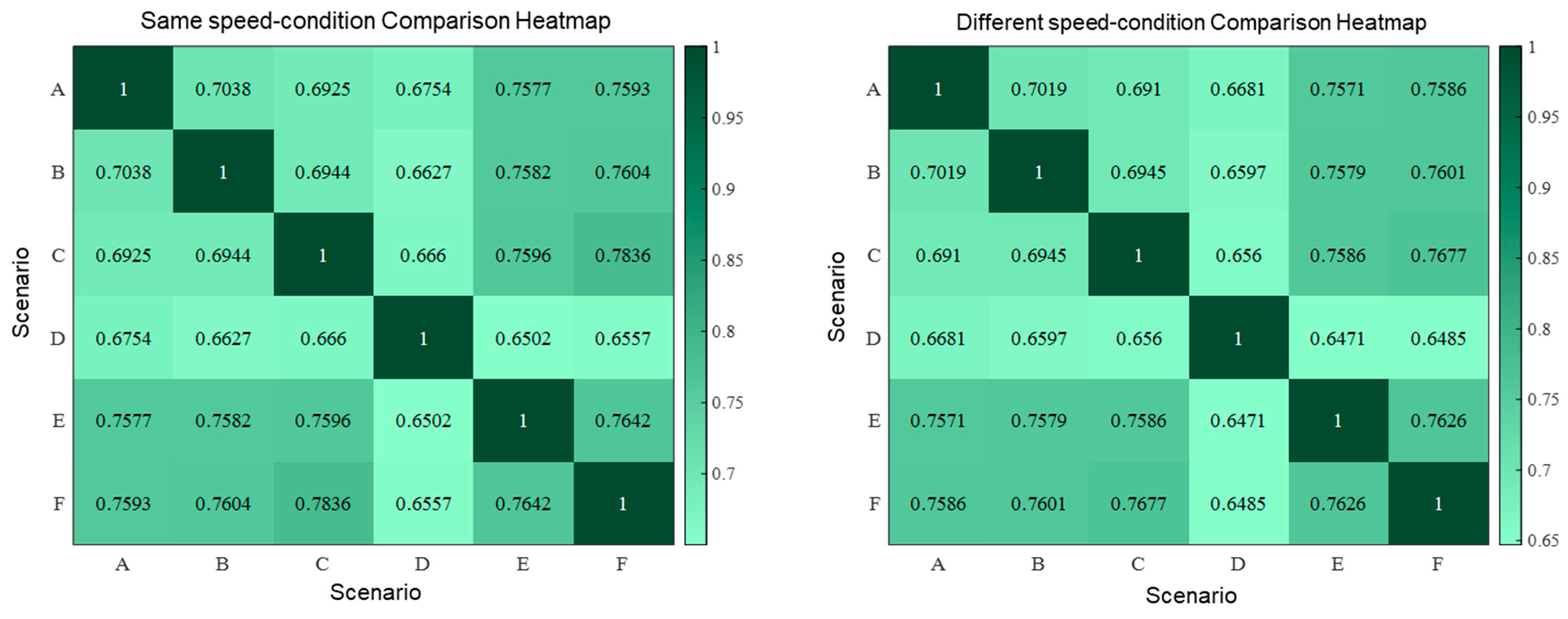
$$S{R}_k^L=\left[D_k^L,A_k^L,C_k^L,A_m^L,C_m^L\right],$$

(54)

$$S{R}_k^M=\left[D_k^M,A_k^M,C_k^M,A_m^M,C_m^M\right],$$

(55)

$$S{R}_k^H=\left[D_k^H,A_k^H,C_k^H,A_m^H,C_m^H\right].$$

(56)

Using $S{R}_k^L, S{R}_k^M$, and $S{R}_k^H$, we quantitatively evaluate the representativeness of a scenario based on its geometric similarity to other scenarios. For this purpose, two comparison methods are proposed: comparison across the same speed condition and comparison across different speed conditions.

The same-speed comparison involves calculating the geometric similarity between different scenarios by comparing the representativeness vectors of each scenario under identical speed conditions. When the number of scenarios is $k$, the number of possible scenario pairs is $\left({\displaystyle \genfrac{}{}{0pt}{}{K}{2}}\right)={\displaystyle \frac{K\left(K-1\right)}{2}}$, and the comparisons are performed across all three speed conditions $\upsilon \in \left\{L,M,H\right\}$ for each scenario pair. The geometric similarity under each speed condition is quantified by comparing the representativeness vectors $S{R}_i^{\upsilon }$ and $S{R}_j^{\upsilon }$ as shown in Equation (57):

$$S{R}_{i,j}^{\mathrm{s}\mathrm{a}\mathrm{m}\mathrm{e}}={\displaystyle \frac{1}{3}}{\sum }_{\upsilon \in V}{y}_S\left({SR}_i^{\upsilon },{SR}_j^{\upsilon }\right).$$

(57)

The different-speed comparison involves evaluating the representativeness of a scenario across different speed conditions, i.e., verifying whether a specific scenario’s representativeness is maintained across various operating conditions. Such an assessment is important for determining the versatility of scenarios. The speed-condition set $\upsilon \in \left\{L,M,H\right\}$ contains six distinct condition pairs $\left({\upsilon }_1,{\upsilon }_2\right), {\upsilon }_1\ne {\upsilon }_2$, and the geometric similarity assessments are performed across all heterogeneous condition pairs for scenario pairs (i,j). Each comparison is designated as $y_S\left({SR}_i^{{\upsilon }_1},{SR}_j^{{\upsilon }_2}\right)$, and the overall different-speed similarity score is calculated as shown in Equation (58):

$$S{R}_{i,j}^{\mathrm{d}\mathrm{i}\mathrm{f}\mathrm{f}\mathrm{e}\mathrm{r}}={\displaystyle \frac{1}{6}}{\sum }_{\begin{array}{c}\upsilon \in V\times V\\ {\upsilon }_1\ne {\upsilon }_2\end{array}}{y}_S\left({SR}_i^{{\upsilon }_1},{SR}_j^{{\upsilon }_2}\right).$$

(58)

Thus, for each pair of scenarios, two comparison scores can be calculated, whereby a total of $\left({\displaystyle \genfrac{}{}{0pt}{}{K}{2}}\right)={\displaystyle \frac{K\left(K-1\right)}{2}}$ individual scenario representativeness scores are obtained for K scenarios. Therefore, the total number of similarity scores is $K(K-1)$. The scenario representativeness scores calculated in this manner are visualized as a heatmap and serve as the basis for selecting representative scenarios for credibility assessment.

5. Field Test Configuration and Results

To validate the proposed credibility evaluation methodology, we conducted a case study on VILS, one of the four main XILS approaches. Specifically, among the various VILS techniques, PG-based VILS was adopted to replicate scenarios that are difficult to implement repeatedly in real-vehicle tests and to capture behavioral characteristics similar to those of actual vehicles. To test the credibility evaluation methodology, we performed PG-based VILS across the six scenarios defined in Section 3.1 (K = 6), which comprised lateral evaluation (A and B), longitudinal evaluation (C and D), and combined longitudinal–lateral evaluation (E and F). For each scenario, both VILS and real-vehicle tests were conducted five times each (N = 5), and the results were measured against the 12 key parameters presented in Table 1 (M = 12). This section describes the vehicle configuration and evaluation environment utilized for the real-world vehicle testing and VILS testing and explains how the credibility of the VILS platform was evaluated based on test results obtained from both real and virtual environments. The procedures to evaluate the verification efficiency and representativeness through geometric similarity calculations are then outlined.

5.1. Experimental Setup

The proposed credibility evaluation methodology for XILS platforms was validated by constructing a VILS environment and comparatively analyzing the VILS results against those from real-world experiments. By repeatedly implementing the same test scenario in both real and virtual environments, we aimed to quantitatively evaluate the credibility and reproducibility of XILS-based verification.

The subject vehicle was a Hyundai Kona (Hyundai Motor Company, Seoul, Republic of Korea) featuring an ADS comprising an integrated controller based on a real-time control unit MicroAutoBox3 (MAB3) (dSPACE GmbH, Paderborn, Germany) equipped with an autonomous driving algorithm. An RT3002-v2 Real-Time Kinematic (RTK) (Oxford Technical Solutions, Oxfordshire, UK)—GPS device was used to ensure precise positioning of the vehicle, and the sensor system for peripheral object and lane recognition was adapted from previous studies by incorporating a multi-sensor fusion method. Specifically, a RoboSense lidar (RoboSense, Shenzhen, China), a Hyundai Mobis radar (Hyundai Mobis, Seoul, Republic of Korea), and a Mobileye 630 camera (Mobileye, Jerusalem, Israel) were integrated to improve recognition performance. The target vehicle was a Hyundai Sonata, which was equipped with a real-time controller MicroAutoBox2 (dSPACE GmbH, Paderborn, Germany) and RTK-GPS sensors featuring the same autonomous driving algorithm. This vehicle was selected to minimize driver intervention and maximize the reproducibility of the scenarios during the repeated experiments, as its cruise control function can consistently maintain a specified route and speed. For precise collection of the experimental data, a Vector VN1640 (Vector Informatik GmbH, Stuttgart, Germany) was used to monitor the CAN messages from the real car and the VILS environment in real time. The logged data were stored in the form of CAN database files, which were utilized for the credibility evaluation. A description and configuration of vehicles and devices is shown in Figure 5.

The real-vehicle tests were conducted at K-City, the autonomous driving testbed of the Korea Automotive Technology Institute (KATRI). As shown in Figure 6, the test facility comprises a curved section approximately 320 m long and having curve radii of 70 m, 80 m, and 70 m, together with a one-way, three-lane straight section of approximately 600 m. These road segments are specifically designed to evaluate both the longitudinal and lateral dynamic characteristics of autonomous vehicles. For the simulation (VILS) experiments, a virtual track with an identical geometry was constructed based on HD-map data. These tests were performed in a designated area of the KATRI proving ground designed to accommodate the target road dimensions. By maintaining the same autonomous driving algorithm and scenario conditions across the real and VILS environments, the credibility of the XILS platform could be quantitatively evaluated.

5.2. Credibility Evaluation Results

The credibility evaluation methodology outlined in Section 3 was employed to quantitatively analyze and compare the results of the real-vehicle tests (Real) and PG-based VILS tests (Sim). Six test scenarios (A–F), each representing a distinct driving behavior, were evaluated from three perspectives: parameter-based, scenario-based, and dynamics-based. Based on the results, we examined how consistently the XILS platform performed in terms of reliability and fidelity, before integrating the findings to assess its overall credibility. Finally, we reviewed the limitations of the evaluation metrics used and their potential scope for enhancement, gaining insights regarding future research directions.

5.2.1. Results of Key Parameter-Based Evaluation

Following the parameter-based reliability evaluation methodology presented in Section 3.2, we comparatively analyzed the results of the real-vehicle (Real) and VILS (Sim) tests across the 12 key parameters listed in

Table 2. Consistency indices of key parameters.

	Parameter	p1	p2	p3	p4	p5	p6	p7	p8	p9	p10	p11	p12
Index
Pm(r)		0.811	0.844	0.886	0.972	0.947	0.852	0.866	0.963	0.902	0.964	0.774	0.867
Pm(v)		0.848	0.868	0.91	0.971	0.961	0.94	0.898	0.963	0.915	0.967	0.924	0.912
Pm(v, r)		0.706	0.746	0.748	0.943	0.877	0.747	0.794	0.922	0.805	0.916	0.683	0.814

. All tests were repeated five times, and the graphs of the real-vehicle data (Real) and VILS data (Sim) are represented by dashed and solid lines, respectively, to ensure an intuitive comparison (Figure 7 and Figure 8).

In Scenario B, the yaw angle ($\psi$), lateral acceleration ($a_y$), yaw rate ($\mathsf{\gamma }$), desired steering angle (${\delta }_{des}$), and driving trajectory ($X, Y$) were analyzed (Figure 7), with the trajectory data being presented in two separate plots [31]. The first plot shows the results of the repeated real-vehicle tests conducted on the actual road, while the second (“synchronized”) plot shows all test runs aligned to the origin (0,0) via rotation and translation. This synchronization is necessary because the VILS tests were performed in multiple areas of the PG environment. Since each area had a different initial position and orientation, the trajectory and yaw angle were both reset to (0,0). The synchronized yaw angle and trajectory plots for the real-vehicle and VILS tests both show a consistent S-shaped pattern; specifically, the two trajectory patterns are nearly identical, which indicates accurate coordinate synchronization. In contrast, some subtle differences are observed between the synchronized yaw graphs, which are attributed to errors during the generation of the virtual road model reflecting the actual road geometry based on the high-precision map. The lateral acceleration, yaw rate, and desired steering angle plots show minor oscillations within each test iteration, attributable to road-surface irregularities and sensor noise during real-world driving. Notably, the yaw rate peak around 30 s appears almost identical between the real-vehicle and VILS tests, which demonstrates that the VILS system accurately replicated the real vehicle’s dynamic maneuvers.

In Scenario C, the longitudinal acceleration ($a_x$), vehicle speed ($V_e$), desired longitudinal acceleration ($a_{x,des}$), relative longitudinal distance ($R{D}_x$), relative lateral distance ($R{D}_y$), and relative velocity ($RV$) were analyzed (Figure 8). The test was conducted from 0 to 35 s, with the subject vehicle and the target vehicle both starting from rest. The subject vehicle reached approximately 15 m/s at around 10 s. The target vehicle performed a cut-in maneuver between 12 and 15 s, causing the relative lateral distance to drop sharply from about 3 m to 0 m. In response, the autonomous driving controller of the subject vehicle issued a deceleration command of about –2.5 m/s². In the desired acceleration plot, the close match between real-vehicle and VILS results confirms that the control algorithm behaved identically in both environments. The relative longitudinal distance plot shows the gap between the vehicles widening during the initial 0–5 s period and then gradually narrowing after the cut-in maneuver, while the relative velocity plot exhibits a peak of about –6 m/s at the cut-in point, indicating that the target vehicle entered the subject vehicle’s lane at a lower speed. The relative lateral distance displayed greater variability during the real-vehicle tests due to initial-position offsets, lane-alignment differences, and sensor-perception errors, whereas the VILS test yielded more consistent results because of the virtual sensor modeling and automated scenario execution.

Table 2 lists the consistency indices of the main test parameters calculated using equations formulated in previous studies [29,30], while

Table 3. Correlation and applicability indices of key parameters, along with evaluation criteria.

	Parameter	p1	p2	p3	p4	p5	p6	p7	p8	p9	p10	p11	p12	Criterion
Index
Cm (%)		88.25	88.39	84.42	97.02	92.61	87.68	91.69	95.74	89.25	95.02	88.24	93.89	76.34 (αP)
Am (%)		106.11	102.84	102.71	99.91	101.48	110.33	103.7	100.12	101.44	100.31	119.38	105.19	83.51 (βP)

presents the correlation and applicability indices calculated using Equations (7) and (8).

Compared with the prior study [31], the ordering of the parameters in this study was different, e.g., our $p_1$ (lateral acceleration) corresponds to $p_8$ in the previous study. Considering this, a particularly noteworthy finding is that, whereas the earlier paper reported a correlation index of 71.8% for $p_8$, thus failing to meet the evaluation criterion (${\alpha }_p$ = 76.3%), we achieved an improved correlation index of approximately 88.25% for p₁. This improvement stems from enhancements to the simulation logic: unlike in the previous study, we automated event triggering (e.g., lane changes) within fixed segments to minimize manual tester intervention, which markedly boosted reproducibility in the lateral performance scenarios. Furthermore, our $p_{12}$ (relative velocity) consolidates $R{V}_x$ and $R{V}_y$ from the prior study into a single parameter. Despite this simplification, this parameter exhibited a high correlation index of 93.89%, which demonstrates the effectiveness of our parameter design. The applicability index ($A_m$) exceeded 100% for all parameters, thereby confirming the superior reproducibility and repeatability of the VILS tests. Specifically, $p_{11}$ (relative lateral distance) exhibited an applicability index of 119.38%, attributable to our improved perception sensor model and virtual traffic generation algorithm.

In summary, the VILS system implemented in this study—improving on the system from the previous research—achieved greater reliability in terms of certain parameters through reduced tester involvement and a more refined automation logic. Given that all parameters satisfied their respective evaluation criteria, the simulation environment for ADS verification can be considered credible.

5.2.2. Results of Scenario-Based Evaluation

The six test scenarios shown in Figure 3 were evaluated using the scenario-based reliability assessment methodology introduced in Section 3.3.

Table 4. Consistency indices for each scenario.

	Scenario	A	B	C	D	E	F
Index
Sk (r)	Low	0.922	0.963	0.942	0.916	0.864	0.846
	Mid	0.895	0.952	0.893	0.88	0.845	0.82
	High	0.873	0.933	0.865	0.848	0.822	0.806
Sk (v)	Low	0.982	0.981	0.972	0.965	0.902	0.852
	Mid	0.965	0.972	0.961	0.952	0.89	0.87
	High	0.943	0.963	0.948	0.935	0.87	0.876
Sk (r, v)	Low	0.883	0.913	0.868	0.884	0.774	0.757
	Mid	0.841	0.894	0.786	0.817	0.737	0.721
	High	0.808	0.851	0.729	0.747	0.681	0.676

lists the consistency indices, with values closer to 1 indicating a higher similarity between the two experiments compared.

Table 5. Correlation and applicability indices for each scenario, along with evaluation criteria.

	Scenario	A	B	C	D	E	F	Criterion
Index
Ck (%)	Low	95.79	94.86	92.11	96.54	89.53	89.43	83.9 (αS)
	Mid	93.96	93.86	88.21	92.81	87.2	87.86	82.8 (αS)
	High	92.49	91.23	84.33	88.09	82.81	83.93	80.7 (αS)
Ak (%)	Low	106.55	101.91	103.14	105.39	104.34	100.69	96.7 (βS)
	Mid	107.77	102.1	107.62	108.17	105.37	105.98	97.1 (βS)
	High	107.95	103.31	109.63	110.37	105.81	108.66	96.9 (βS)

presents the correlation and applicability indices for each test scenario. According to the data in Table 4, the inter-repetition consistency indices of the VILS tests generally exceeded those of the real-vehicle tests across all scenarios. This indicates that the VILS tests could reproduce the same scenario with higher precision and repeatability, which highlights their advantage over real-vehicle tests in terms of reproducibility and consistency within a simulation environment.

However, the consistency index between the real-vehicle and VILS tests was slightly lower than the consistency index within each testing environment. This implies that within the same experimental configuration, structural differences between the two platforms, along with input errors, affected the consistency between the corresponding results. These observations indicate inherent differences between real-world environments and simulation environments. Notably, Scenarios E and F exhibited lower consistency indices than the other scenarios. This is because these scenarios include both longitudinal and lateral vehicle behavior, which restricts the possibility of achieving consistent results.

Another important pattern in Table 4 is the variation in the consistency index according to the speed condition. In all scenarios, the consistency indices displayed a clear decreasing trend with increasing speed. Specifically, the inter-repetition consistency index for the real-vehicle tests decreased from 0.922 under the low-speed condition to 0.873 under the high-speed condition in Scenario A, and from 0.846 to 0.806 in Scenario F. This reflects the physical phenomenon in which maintaining consistency in vehicle behavior becomes more difficult as speed increases, because factors such as inertial forces, tire dynamics, and steering sensitivity interact more complexly, resulting in greater variability in system responses to the same inputs. Additionally, the consistency indices for Scenarios C and D were lower than those for Scenarios A and B; this shows that the inclusion of the target vehicle increased the structural complexity of the scenarios, whereby ensuring consistency in system responses between repeated experiments became more difficult. The consistency index between the real-vehicle and VILS tests was also significantly lower in the integrated behavior scenarios (E and F) than in the single-behavior scenarios (A–D). Particularly under the high-speed condition, Scenarios E and F recorded the lowest values, at 0.681 and 0.676, respectively. This reflects the increasing difficulty in ensuring coherent multi-dimensional system responses due to the inclusion of both longitudinal and lateral terms in the main parameters used for the consistency index calculations.

Table 5 presents the correlation index and applicability index for each scenario as percentages, with all metrics meeting the pre-established criteria across all scenarios. Notably, the applicability index exceeded 100% in all scenarios and under all speed conditions. This numerically verifies that the VILS tests were more repeatable and reproducible than the real-vehicle tests, indicating that the VILS environment was sufficiently reliable to replace real-vehicle testing. Under the high-speed condition in Scenario D, the applicability index recorded its highest value (110.37%), which suggests that VILS tests can provide more consistent results than real-vehicle tests even in complex and challenging driving situations. The correlation index also exhibited a consistent pattern with respect to the speed condition, displaying a decreasing trend with increasing speed across all scenarios. In Scenario A, the correlation index decreased from 95.79% under the low-speed condition to 92.49% under the high-speed condition, while in Scenario E, it underwent a larger reduction, from 89.53% to 82.81%. This observation can be interpreted as the dynamic differences between real and simulated vehicles becoming more pronounced in higher-speed driving situations. Interestingly, the single-behavior scenarios (A–D) showed higher correlation indices than the integrated-behavior scenarios (E and F), which suggests that VILS environments can be more coherent in relatively simple scenarios. Conversely, the applicability index tended to be higher in more complex scenarios and under higher-speed conditions. Under the high-speed condition in Scenario D, it recorded its highest value (110.37%), which signifies that the VILS tests were more consistent than the real-vehicle tests under more complex conditions.

5.2.3. Results of Dynamics-Based Evaluation

We comparatively analyzed each scenario using the dynamics-based fidelity assessment methodology described in Section 3.4. The similarity of the dynamic motion responses between VILS and real-vehicle tests was quantitatively analyzed based on the six DOFs that constitute the translational and rotational motions of a vehicle.

Table 6. Dynamics-based consistency index for each scenario.

	Scenario	A	B	C	D	E	F
Index
Dk (r)	Low	0.880	0.887	0.728	0.781	0.711	0.703
	Mid	0.853	0.854	0.711	0.752	0.684	0.673
	High	0.814	0.818	0.668	0.721	0.658	0.644
Dk (v)	Low	0.924	0.931	0.769	0.825	0.753	0.756
	Mid	0.892	0.899	0.74	0.796	0.724	0.725
	High	0.854	0.865	0.709	0.764	0.697	0.697
Dk (r, v)	Low	0.741	0.743	0.571	0.636	0.54	0.539
	Mid	0.718	0.713	0.542	0.608	0.514	0.511
	High	0.683	0.676	0.511	0.577	0.491	0.483

lists the dynamic consistency indices calculated by weighting the average similarity index for each DOF. Values closer to 1 indicate more consistent dynamic responses between the simulated and real vehicles.

Table 7. Dynamics-based correlation for each scenario, along with evaluation criteria.

	Scenario	A	B	C	D	E	F	Criterion
Index
Dk (%)	Low	84.205	83.766	78.434	81.434	75.949	76.671	68.6 (αD)
	Mid	84.174	83.489	77.429	80.851	75.146	75.929	65.62 (αD)
	High	83.907	82.641	76.497	80.028	74.468	75.127	62.55 (αD)

presents the dynamic correlation index for each scenario.

The dynamics consistency index and correlation values in Table 6 and Table 7 exhibit a clear pattern. Across all scenarios, the consistency index and correlation displayed a consistent, gradually decreasing trend with increasing speed. This is ascribed to the increased influence of disturbances such as crosswinds and road surface irregularities, which are more pronounced at higher speeds, along with amplified nonlinearities in the tire–body dynamics and increased input–output timing differences due to controller response delays. In terms of the evaluation type, the best dynamic consistency was observed within the VILS tests, while relatively low consistency was observed between the real-world and VILS tests. This is attributed to the structural advantage of the simulation environment, which allows precise control over the initial conditions. Regarding the effect of scenario complexity, the lateral-motion scenarios (A and B) exhibited the highest consistency index, the longitudinal-motion scenarios (C and D) displayed moderate consistency, and the integrated scenarios (E and F) showed the lowest consistency. The low consistency in the integrated scenarios resulted from the complex response of the system due to the simultaneous occurrence of longitudinal and lateral inputs and the dynamic interaction between the subject and target vehicles.

The foregoing observations underscore the advantages of the proposed dynamics-based fidelity assessment over traditional assessment methods. First and foremost is the ability to reflect disturbances. Our method can compare the reproducibility between real-world and simulation tests, considering various disturbance factors, such as crosswinds, road surface conditions, and tire characteristics, an important aspect that is often overlooked in traditional parameter-based evaluations. Additionally, the dynamics evaluation utilizes a multidimensional measurement mechanism: rather than depending on a single parameter or a specific input condition, it integrally measures the complex response of the overall system, thereby mitigating structural inconsistencies. This results in a balanced distribution of the dynamics correlation indices, without extremes. In terms of practical credibility, the evaluation criterion $\left({\alpha }_D\right)$ being satisfied in all scenarios and under all speed conditions proves that the VILS platform could adequately reproduce the real vehicle’s dynamics, even in complex, integrated-behavior scenarios.

The dynamics-based fidelity assessment is superior to existing methodologies as it includes vehicle dynamics characteristics. Existing evaluation metrics focus only on individual parameters or scenario-related results and do not comprehensively reflect the dynamics of the vehicle. In contrast, the proposed dynamics-based methodology ensures a comprehensive evaluation by measuring the dynamic response of the entire vehicle system. The consideration of real-time control feedback represents another important advantage. The dynamics-based evaluation includes the vehicle control system feedback loops, as well as their time delays and nonlinear response characteristics. This is particularly important under high-speed conditions or in complex scenarios as it enables a systematic analysis of uncertainty factors.

Despite the merits of the proposed methodology, considering the results of our evaluation, specific aspects of the framework can be improved to strengthen the credibility assessment of the VILS platform further. The most important enhancement would be the incorporation of a highly accurate, real-world-based tire–road interaction model. A tire model that accurately simulates the physical properties and behavior of real tires is necessary, as is using high-resolution road-profile data to simulate actual road surface conditions more accurately. The input response of the high-speed area control must be synchronized better as well. Algorithms must be developed to compensate for the time delays and nonlinearities that occur during high-speed driving. Delay compensation within the controller is another important requirement, which necessitates the introduction of compensation techniques to minimize the difference in control signal delay between the real vehicle and the simulated vehicle. The credibility of the evaluation can be improved further by extending the experimental conditions to cover more types of driving situations. Moreover, the statistical analysis should be strengthened with additional scenarios, speed conditions, and experimental trials. Specifically, the scope of the evaluation must be expanded by adding variables such as extreme weather conditions.

Overall, we comprehensively validated the credibility of the VILS platform through parameter-based and scenario-based reliability evaluations and a dynamics-based fidelity evaluation. In particular, the dynamics-based fidelity evaluation captured the various disturbances and vehicle dynamics characteristics encountered in real-world driving environments, demonstrating the potential of virtual-environment testing to replace real-world testing. Our integrated evaluation methodology can serve as a dependable validation framework during the development of ADSs and ADASs, ultimately helping address the technical limitations and social acceptance issues surrounding the commercialization of autonomous driving technologies.

5.3. Results of Geometric Similarity Evaluation

We analyzed the testing efficiency and scenario representativeness based on the geo 장어metric similarity indicators presented in Section 4. For the scenarios that were deemed credible based on the three evaluation criteria discussed earlier, we calculated the geometric similarity between the shapes by visualizing the credibility-assessment results across the three representative speed ranges—low, medium, and high—through spider charts. The aim of this process was to quantify the consistency of shape changes across speed conditions and verify whether the results for a specific speed condition can represent the characteristics across the entire speed range.

The primary objective of this study was to establish objective criteria for determining whether testing under a single representative speed condition can replace individual tests under multiple speed conditions when the speed condition is not a dominant factor in the credibility assessment. This approach can significantly enhance testing efficiency and resource optimization if the geometric similarity between velocity conditions exceeds a certain threshold. Section 5.3.1 and Section 5.3.2 present the results of the geometric similarity assessment and the scenario representativeness assessment, respectively. Through a multifaceted interpretation and in-depth examination of these results, we discuss the efficiency and validity of the geometry-based verification methodology.

5.3.1. Results of Efficiency Evaluation

The geometric similarity vectors for each speed condition in each test scenario were defined using Equations (41)–(43). Based on these vectors, we quantitatively analyzed the geometric similarity between the two shapes depicted in the spider charts to determine the testing efficiency during credibility evaluation. To evaluate the consistency of the differences between the shapes corresponding to the different speed conditions, we utilized vector components based on the three previously derived metrics: dynamics-based correlation $\left(D_k\right)$, scenario-based applicability $\left(A_k\right)$, and scenario-based correlation $\left(C_k\right)$.

Table 8. Geometric similarity vector components for each scenario.

Scenario A					Scenario B					Scenario C
	${\mathit{Y}}_{\mathit{A}}$	${\mathit{D}}_{\mathit{k}}$	${\mathit{A}}_{\mathit{k}}$	${\mathit{C}}_{\mathit{k}}$		${\mathit{Y}}_{\mathit{B}}$	${\mathit{D}}_{\mathit{k}}$	${\mathit{A}}_{\mathit{k}}$	${\mathit{C}}_{\mathit{k}}$		${\mathit{Y}}_{\mathit{C}}$	${\mathit{D}}_{\mathit{k}}$	${\mathit{A}}_{\mathit{k}}$	${\mathit{C}}_{\mathit{k}}$
Speed					Speed					Speed
Low		83.92	106.55	95.79	Low		83.77	101.91	94.86	Low		78.43	103.14	92.11
Mid		84.17	107.77	93.96	Mid		83.49	102.1	93.86	Mid		77.43	107.62	88.21
High		83.91	107.95	92.49	High		82.64	103.31	91.23	High		76.5	109.63	84.33
Scenario D					Scenario E					Scenario F
	${\mathit{Y}}_{\mathit{D}}$	${\mathit{D}}_{\mathit{k}}$	${\mathit{A}}_{\mathit{k}}$	${\mathit{C}}_{\mathit{k}}$		${\mathit{Y}}_{\mathit{E}}$	${\mathit{D}}_{\mathit{k}}$	${\mathit{A}}_{\mathit{k}}$	${\mathit{C}}_{\mathit{k}}$		${\mathit{Y}}_{\mathit{F}}$	${\mathit{D}}_{\mathit{k}}$	${\mathit{A}}_{\mathit{k}}$	${\mathit{C}}_{\mathit{k}}$
Speed					Speed					Speed
Low		81.43	105.39	96.54	Low		75.95	104.34	89.53	Low		76.67	100.69	89.43
Mid		80.85	108.17	92.81	Mid		75.15	105.37	87.2	Mid		75.93	105.98	87.86
High		80.03	110.37	88.09	High		74.47	105.8	82.81	High		75.13	108.66	83.93

summarizes the values of $D_k$, $A_k$, and $C_k$ for Scenarios A–F, which were used as input vectors to compare the geometric shapes on the spider charts. Figure 9 presents the triangular spider charts constructed based on these vectors, which provide an intuitive visualization of the geometric characteristics and variation patterns corresponding to each speed condition in each scenario.

The similarities between these shapes were quantitatively assessed based on the Procrustes, Fréchet, and Hausdorff distance metrics introduced earlier; these metrics were calculated using Equations (37)–(39), respectively, and captured different geometric characteristics, allowing for complementary evaluations. The geometric similarity index $\left(G_k\right)$ was then derived via a weighted integration of the three distance measures based on Equation (44).

Table 9. Geometric similarity for each scenario, along with evaluation criteria.

	Scenario	A	B	C	D	E	F	Criterion
Index
${\mathit{G}}_{\mathit{k}}$ (%)		81.11	80.86	76.09	75.43	78.09	76.52	71.68 (αG)

lists the scores calculated accordingly for each scenario.

The analysis confirms that the geometric similarity indices for all scenarios significantly exceeded the evaluation criterion (71.68%), thereby statistically validating the morphological consistency across speed conditions within each scenario. This indicates that speed is not a dominant factor in credibility assessment, suggesting that independent credibility evaluations for different speed conditions within a given test scenario are unnecessary. Representative speed conditions can sufficiently capture the essential characteristics of any scenario, thus enhancing testing efficiency considerably.

However, notably different patterns emerged across the distinct scenario types. The lateral-motion scenarios (A and B) exhibited high similarity indices (81.11% and 80.86%, respectively), while the longitudinal-motion scenarios (C and D) recorded relatively lower indices (76.09% and 75.43%, respectively). These differences reflect the fundamental characteristics of vehicle dynamics.

The high similarity observed in the lateral-motion scenarios is attributed to the fact that lateral motions, such as lane changes or curve driving, primarily depend on the proportional relationships between yaw rate, lateral acceleration, and steering angle. These relationships are influenced more by the vehicle’s fundamental structure and tire characteristics than by speed changes. Additionally, under normal driving conditions, the tires operate within their linear response range, maintaining similar response characteristics at different speeds.

Conversely, the lower similarity in the longitudinal-motion scenarios stems from physical characteristics related to acceleration and deceleration. As speed increases, the air resistance increases drastically, in proportion to the square of the speed, whereas the rolling resistance increases gradually, in proportion to speed. Furthermore, powertrain efficiency varies complexly with speed. Particularly at low speeds, the engine output is more sensitive to the vehicle’s inertia, whereas at high speeds, it is affected more by the air resistance and control system delays. These factors increase the speed sensitivity of the vehicle’s longitudinal behavior, resulting in the relatively low similarity indices observed.

Notably, the integrated scenarios showed higher similarity indices than the longitudinal-motion scenarios, contrary to expectations. This is ascribed to the complementary nature of the complex vehicle behaviors. When longitudinal and lateral movements occur simultaneously, the extreme characteristics in each direction balance each other out, and complex movements trigger the intervention of the vehicle’s stability control systems; thus, consistent movement is maintained despite speed variations. This inference highlights a paradoxical complexity–stability relationship, where single-behavior scenarios are more sensitive to speed changes than integrated-behavior scenarios, contradicting the general logic that system stability decreases with increasing complexity.

The geometric similarity indices satisfying their respective evaluation criteria across all scenarios suggest that the credibility of the simulation platform within a given scenario could be assessed under a single representative speed condition. Thus, the proposed geometric similarity-based framework can considerably streamline the credibility verification process for XILS platforms.

In summary, while all scenarios maintained adequate similarity across speed conditions, they exhibited distinct patterns correlated with vehicle dynamics principles. Based on this understanding, strategies can be developed to optimize testing efficiency while maintaining the credibility of XILS platforms.

5.3.2. Results of Scenario Representativeness Evaluation

To determine whether a specific scenario can represent other scenarios, we evaluated the similarity between different scenarios. To this end, we calculated the parameter applicability index $\left(A_m\right)$ and correlation index $\left(C_m\right)$ for different speeds using Equations (51)–(53) (Section 4.2) and visualized them in a spider chart along with the dynamic correlation index $\left(D_k\right)$, scenario-based applicability index $\left(A_k\right)$, and scenario-based correlation index $\left(C_k\right)$.

Table 10. Scenario representativeness vector components for each scenario.

Scenario A							Scenario B
	${\mathit{S}\mathit{R}}_{\mathit{A}}$	${\mathit{D}}_{\mathit{k}}$	${\mathit{A}}_{\mathit{k}}$	${\mathit{C}}_{\mathit{k}}$	${\mathit{A}}_{\mathit{m}}$	${\mathit{C}}_{\mathit{m}}$		${\mathit{S}\mathit{R}}_{\mathit{B}}$	${\mathit{D}}_{\mathit{k}}$	${\mathit{A}}_{\mathit{k}}$	${\mathit{C}}_{\mathit{k}}$	${\mathit{A}}_{\mathit{m}}$	${\mathit{C}}_{\mathit{m}}$
Speed							Speed
Low		84.484	101.748	96.985	104.969	98.731	Low		85.255	101.829	95.466	103.127	95.9041
Mid		83.292	105.694	100.133			Mid		83.313	102.560	97.327
High		81.164	106.667	98.915			High		79.985	103.883	95.019
Scenario C							Scenario D
	${\mathit{S}\mathit{R}}_{\mathit{C}}$	${\mathit{D}}_{\mathit{k}}$	${\mathit{A}}_{\mathit{k}}$	${\mathit{C}}_{\mathit{k}}$	${\mathit{A}}_{\mathit{m}}$	${\mathit{C}}_{\mathit{m}}$		${\mathit{S}\mathit{R}}_{\mathit{D}}$	${\mathit{D}}_{\mathit{k}}$	${\mathit{A}}_{\mathit{k}}$	${\mathit{C}}_{\mathit{k}}$	${\mathit{A}}_{\mathit{m}}$	${\mathit{C}}_{\mathit{m}}$
Speed							Speed
Low		83.957	102.175	95.312	103.555	95.442	Low		82.347	102.071	99.615	104.164	96.807
Mid		81.028	103.658	96.619			Mid		81.001	103.440	96.588
High		77.907	104.417	94.871			High		79.076	105.617	94.511
Scenario E							Scenario F
	${\mathit{S}\mathit{R}}_{\mathit{E}}$	${\mathit{D}}_{\mathit{k}}$	${\mathit{A}}_{\mathit{k}}$	${\mathit{C}}_{\mathit{k}}$	${\mathit{A}}_{\mathit{m}}$	${\mathit{C}}_{\mathit{m}}$		${\mathit{S}\mathit{R}}_{\mathit{F}}$	${\mathit{D}}_{\mathit{k}}$	${\mathit{A}}_{\mathit{k}}$	${\mathit{C}}_{\mathit{k}}$	${\mathit{A}}_{\mathit{m}}$	${\mathit{C}}_{\mathit{m}}$
Speed							Speed
Low		80.639	101.745	90.050	102.893	88.065	Low		83.487	104.545	94.565	106.668	92.893
Mid		76.774	102.700	88.956			Mid		79.644	105.278	94.997
High		75.816	103.936	87.361			High		78.682	106.890	92.077

summarizes the scenario representativeness vectors for each test scenario. Based on these multidimensional vectors, we performed two types of comparison: the same-speed comparison focused on the geometric similarity between scenarios under the same speed conditions (low, medium, or high), while the different-speed-condition comparison involved evaluating the geometric similarity between scenarios across different speed conditions (low–medium, medium–high, and high–low) to systematically determine the generalizability of representative scenarios across speed ranges. The results of this comparison are summarized in

Table 11. Scenario representativeness index within and across speed conditions.

	Scenario	A:B	A:C	A:D	A:E	A:F	B:C	B:D	B:E	B:F	C:D	C:E	C:F	D:E	D:F	E:F
Condition
Same speed		0.704	0.692	0.675	0.758	0.759	0.694	0.663	0.758	0.76	0.666	0.76	0.784	0.65	0.656	0.764
Different speed		0.702	0.691	0.668	0.757	0.759	0.695	0.66	0.758	0.76	0.656	0.759	0.768	0.647	0.649	0.763

and presented as heat maps in Figure 10. Figure 11 provides an intuitive visualization of the same results through spider charts.

The similarity indices across most scenario combinations showed minimal differences in both the same-speed and different-speed comparisons. This can be interpreted in two ways. First, the inherent dynamic characteristics of a scenario influence the similarity index more than speed changes. This suggests the possibility of using representative scenarios for testing across various speed conditions. Second, the slightly higher similarity observed in the same-speed comparisons quantitatively demonstrates that speed changes cause small geometric deformations in the scenario characteristics. While these differences were not statistically significant within the range of the test data used in this study, they could be amplified under extreme conditions, such as high-speed driving; this highlights the need for experimental validation across a wider range of speeds.

The results reveal high similarity scores in Scenarios E and F, which must be interpreted based on the fundamental principles of vehicle dynamics. Integrated scenarios include complex interactions between lateral and longitudinal behaviors, inducing situations where extreme changes in individual behaviors offset each other. This phenomenon allows integrated scenarios to maintain substantial similarity to single-behavior scenarios. Thus, integrated scenarios reflect characteristics emerging from dynamic interactions rather than simply being arithmetic combinations of individual behaviors.

The consistently low similarity index for Scenario D has important theoretical and practical implications. It reflects the fundamental characteristic that longitudinal behavior is more sensitive to speed changes than other behaviors, a phenomenon stemming from the nonlinearity of vehicle dynamics. Longitudinal following behavior is governed by nonlinear relationships between relative speed, acceleration, and any resulting braking and acceleration control inputs. Speed variations amplify this nonlinearity, significantly deforming the relevant geometric shapes within the parameter space. In contrast, lateral behavior maintains relatively stable geometric patterns because the associated steering control characteristics are less sensitive to speed changes. Therefore, Scenario D requires a more systematic verification approach than a single representative scenario. Particularly in high-speed driving situations, longitudinal following behavior may show markedly different characteristics from low-speed driving, necessitating testing under separate conditions for each speed range to verify representativeness. This inference suggests that the safety and performance characteristics of the longitudinal control algorithms in ADSs may depend on the speed condition.

The geometric similarity evaluation methodology proposed herein must be scaled up to achieve comprehensive ADS validation. Specifically, to confirm the representativeness of scenarios, expanded experiments across wider speed ranges and various environmental conditions (road friction, weather, and traffic density) must be conducted. For speed-sensitive behaviors, such as in Scenario D, a more systematic analysis of geometric similarity based on various speed conditions within the same scenario must be performed before evaluating the representativeness of the scenario.

In future research, the correlation between geometric similarity and actual ADS behavior should be examined to determine whether ADSs demonstrate similar safety and performance characteristics in scenarios with high similarity indices. This will provide important insights for evaluating the credibility and efficiency of XILS platforms. The results of this study have practical implications for ADS verification frameworks, suggesting that verification systems centered on integrated-behavior scenarios are more efficient and comprehensive than those based on single-behavior scenarios. Based on geometric similarities between scenarios, we highlighted the possibility of optimizing testing procedures by selecting a minimal set of representative scenarios that reflect the characteristics of various other scenarios. However, since this research included limited conditions, the generalizability of the findings must be strengthened through expanded experiments reflecting more diverse driving situations and environmental variables.

6. Conclusions

Herein, we proposed an integrated verification framework to comprehensively evaluate the credibility of XILS platforms for ADS validation. Through parameter-based and scenario-based evaluations, we quantitatively demonstrated the correlation between VILS and real-vehicle tests and their applicability. Additionally, we introduced a dynamics-based evaluation method, which enables an integrated credibility assessment of the VILS platform. Accordingly, the platform can be deemed credible if it satisfies specific evaluation criteria for parameter-based reliability, scenario-based reliability, and dynamics-based fidelity indicators.

After conducting the credibility assessment, we visualized each evaluation indicator through spider charts and performed similarity evaluations using three geometric indicators: the Procrustes, Fréchet, and Hausdorff distance metrics. Thus, we empirically demonstrated that for a given scenario, credibility can be verified under specific representative speed conditions rather than individually testing all velocity conditions. Furthermore, through geometric similarity evaluations between different scenarios, we highlighted the possibility that an integrated behavior scenario could represent certain other scenarios for credibility evaluation.

Nevertheless, the experiments in this study covered limited scenarios, driving situations, and velocity conditions. To provide clearer guidance for future research and strengthen the generalizability of the proposed framework, several essential areas warrant further investigation: (1) Environmental scenarios including urban traffic environments with complex intersections and pedestrian interactions, highway scenarios with high-speed merging and convoy driving, and adverse weather conditions such as rain, fog, snow, and varying road surface friction that significantly affect vehicle dynamics and sensor performance; (2) operational conditions encompassing extreme speed ranges (very low speeds < 10 km/h for parking scenarios and high speeds > 120 km/h for highway scenarios), sensor degradation and failure modes including partial occlusion and noise interference, and edge cases such as construction zones and emergency vehicle interactions. These expanded experimental conditions would provide a more comprehensive validation framework and enhance the statistical significance of the geometric similarity analysis across diverse operational domains. Therefore, future studies should pursue credibility verification across these diverse and challenging scenarios to fully validate the robustness and applicability of the proposed methodology.

In conclusion, the proposed framework provides a standardized platform for XILS-based ADS verification. The integrated credibility evaluation and geometric similarity evaluation methodologies are expected to facilitate the commercialization of safe autonomous driving technology by improving the efficiency of systematic verification processes.

References

1. Zheng, K.; Fu, J.; Liu, X. Relay Selection and Deployment for NOMA Enabled Multi-UAV-assisted WSN. IEEE Sens. J. 2025, 25, 16235–16249. [Google Scholar] [CrossRef]
2. Li, H.; Makkapati, V.P.; Wan, L.; Tomasch, E.; Hoschopf, H.; Eichberger, A. Validation of automated driving function based on the Apollo platform: A milestone for simulation with vehicle-in-the-loop testbed. Vehicles 2023, 5, 718–731. [Google Scholar] [CrossRef]
3. Issler, M.; Goss, Q.; Akbaş, M.İ. Complexity evaluation of test scenarios for autonomous vehicle safety validation using information theory. Information 2024, 15, 772. [Google Scholar] [CrossRef]
4. Hejase, M.; Özgüner, U.; Barbier, M.; Ibáñez-Guzmán, J. A methodology for model-based validation of autonomous vehicle systems. In Proceedings of the 2020 IEEE Intelligent Vehicles Symposium (IV), Las Vegas, NV, USA, 19–23 October 2020; pp. 2097–2103. [Google Scholar] [CrossRef]
5. Zhang, Q.; Yang, X.J.; Robert, L.P., Jr. Drivers’ age and automated vehicle explanations. Sustainability 2021, 13, 1948. [Google Scholar] [CrossRef]
6. Marti, P.; Jallais, C.; Koustanaï, A.; Guillaume, A.; Mars, F. Impact of the driver’s visual engagement on situation awareness and takeover quality. Transp. Res. Part F Traffic Psychol. Behav. 2022, 87, 391–402. [Google Scholar] [CrossRef]
7. Sainz, I.; Arteta, B.; Coupeau, A.; Prieto, P. X-in-the-loop simulation environment for electric vehicles ECUs. In Proceedings of the 2021 IEEE Vehicle Power and Propulsion Conference (VPPC), Gijón, Spain, 25–28 October 2021; pp. 1–6. [Google Scholar] [CrossRef]
8. Landersheim, V.; Jurisch, M.; Bartolozzi, R.; Stoll, G.; Möller, R.; Atzrodt, H. Simulation-Based Testing of Subsystems for Autonomous Vehicles at the Example of an Active Suspension Control System. Electronics 2022, 11, 1469. [Google Scholar] [CrossRef]
9. Weiss, E.; Gerdes, J.C. High speed emulation in a vehicle-in-the-loop driving simulator. IEEE Trans. Intell. Veh. 2022, 8, 1826–1836. [Google Scholar] [CrossRef]
10. Fayazi, S.A.; Vahidi, A.; Luckow, A. A vehicle-in-the-loop (VIL) verification of an all-autonomous intersection control scheme. Transp. Res. Part C Emerg. Technol. 2019, 107, 193–210. [Google Scholar] [CrossRef]
11. Chen, Y.; Chen, S.; Zhang, T.; Zhang, S.; Zheng, N. Autonomous vehicle testing and validation platform: Integrated simulation system with hardware in the loop. In Proceedings of the 2018 IEEE Intelligent Vehicles Symposium (IV), Changshu, China, 26–30 June 2018; pp. 949–956. [Google Scholar] [CrossRef]
12. Li, C.; Jiang, H.; Yang, X.; Wei, Q. Path Tracking Control Strategy Based on Adaptive MPC for Intelligent Vehicles. Appl. Sci. 2025, 15, 5464. [Google Scholar] [CrossRef]
13. Fu, D.; Zhong, N.; Han, X.; Cai, P.; Wen, L.; Mao, S.; Qiao, Y. LimSim series: An autonomous driving simulation platform for validation and enhancement. arXiv 2025, arXiv:2502.09170. [Google Scholar] [CrossRef]
14. Zhao, X.; Chen, H.; Li, H.; Li, X.; Chang, X.; Feng, X.; Chen, Y. Development and application of connected vehicle technology test platform based on driving simulator: Case study. Accid. Anal. Prev. 2021, 161, 106330. [Google Scholar] [CrossRef] [PubMed]
15. Cheng, J.; Wang, Z.; Zhao, X.; Xu, Z.; Ding, M.; Takeda, K. A survey on testbench-based vehicle-in-the-loop simulation testing for autonomous vehicles: Architecture, principle, and equipment. Adv. Intell. Syst. 2024, 6, 2300778. [Google Scholar] [CrossRef]
16. Park, C.; Chung, S.; Lee, H. Vehicle-in-the-loop in global coordinates for advanced driver assistance system. Appl. Sci. 2020, 10, 2645. [Google Scholar] [CrossRef]
17. Fayazi, S.A.; Vahidi, A. Vehicle-in-the-loop (VIL) verification of a smart city intersection control scheme for autonomous vehicles. In Proceedings of the 2017 IEEE Conference on Control Technology and Applications (CCTA), Maui, HI, USA, 27–30 August 2017; pp. 1575–1580. [Google Scholar] [CrossRef]
18. Chen, Y.; Chen, S.; Xiao, T.; Zhang, S.; Hou, Q.; Zheng, N. Mixed test environment-based vehicle-in-the-loop validation—A new testing approach for autonomous vehicles. In Proceedings of the 2020 IEEE Intelligent Vehicles Symposium (IV), Las Vegas, NV, USA, 19–23 October 2020; pp. 1283–1289. [Google Scholar] [CrossRef]
19. Chen, L.; Xie, J.; Wu, S.; Guo, F.; Chen, Z.; Tan, W. Validation of vehicle driving simulator from perspective of velocity and trajectory based driving behavior under curve conditions. Energies 2021, 14, 8429. [Google Scholar] [CrossRef]
20. United Nations Economic Commission for Europe. Proposal for a New UN Regulation on Uniform Provisions Concerning the Approval of Vehicles with Regard to Driver Control Assistance Systems (DCAS); ECE/TRANS/WP.29/2024/37; Economic Commission for Europe: Geneva, Switzerland, 2024. [Google Scholar]
21. Wynne, R.A.; Beanland, V.; Salmon, P.M. Systematic review of driving simulator validation studies. Saf. Sci. 2019, 117, 138–151. [Google Scholar] [CrossRef]
22. Keil, R.; Tschorn, J.A.; Tümler, J.; Altinsoy, M.E. Evaluation of SiL testing potential—Shifting from HiL by identifying compatible requirements with vECUs. Vehicles 2024, 6, 920–948. [Google Scholar] [CrossRef]
23. Sathyamangalam Imran, M.I.I.; Awasthi, S.S.; Khayyat, M.; Arrigoni, S.; Braghin, F. Virtual Validation and Uncertainty Quantification of an Adaptive Model Predictive Controller-Based Motion Planner for Autonomous Driving Systems. Future Transp. 2024, 4, 1537–1558. [Google Scholar] [CrossRef]
24. Keil, R.; Tschorn, J.A.; Tümler, J.; Altinsoy, M.E. Optimization of Automotive Software Tests by Simplification of the Bus Simulation. In Proceedings of the 2023 IEEE International Workshop on Metrology for Automotive (MetroAutomotive), Modena, Italy, 28–30 June 2023; pp. 72–77. [Google Scholar] [CrossRef]
25. Qiu, W.; Ashta, S.; Shaver, G.M.; Johnson, S.C.; Frushour, B.C.; Rudolph, K. Expediting Hybrid Electric Wheel Loader Prototyping: Real-Time Dynamic Modeling and Power Management Through Advanced Hardware-in-the-Loop Simulation. IEEE Trans. Veh. Technol. 2025, 74, 2682–2691. [Google Scholar] [CrossRef]
26. Abboush, M.; Bamal, D.; Knieke, C.; Rausch, A. Hardware-in-the-loop-based real-time fault injection framework for dynamic behavior analysis of automotive software systems. Sensors 2022, 22, 1360. [Google Scholar] [CrossRef]
27. Wang, Z.; Zha, J.; Wang, J. Autonomous vehicle trajectory following: A flatness model predictive control approach with hardware-in-the-loop verification. IEEE Trans. Intell. Transp. Syst. 2020, 22, 5613–5623. [Google Scholar] [CrossRef]
28. Xia, C.; Zheng, C.; Xia, Y.; Kong, X.; Song, X. Survey on Simulation Testing of Autonomous Driving System. In Proceedings of the 2024 11th International Conference on Dependable Systems and Their Applications (DSA), Taicang, China, 2–3 November 2024; pp. 221–229. [Google Scholar] [CrossRef]
29. Son, W.; Ha, Y.; Oh, T.; Woo, S.; Cho, S.; Yoo, J. PG-based vehicle-in-the-loop simulation for system development and consistency validation. Electronics 2022, 11, 4073. [Google Scholar] [CrossRef]
30. Oh, T.; Ha, Y.; Yoo, D.; Yoo, J. AD-VILS: Implementation and reliability validation of vehicle-in-the-loop simulation platform for evaluating autonomous driving systems. IEEE Access 2024, 12, 164190–164209. [Google Scholar] [CrossRef]
31. Oh, T.; Cho, S.; Yoo, J. A reliability evaluation methodology for X-in-the-loop simulation in autonomous vehicle systems. IEEE Access 2024, 12, 193622–193640. [Google Scholar] [CrossRef]
32. Mongiardini, M.; Ray, M.; Anghileri, M. Acceptance criteria for validation metrics in roadside safety based on repeated full-scale crash tests. Int. J. Reliab. Saf. 2010, 4, 69–89. [Google Scholar] [CrossRef]
33. Ray, M.H.; Mongiardini, M.; Plaxico, C. Quantitative methods for assessing similarity between computational results and full-scale crash tests. In Proceedings of the 91st Annual Meeting of the Transportation Research Board, Washington, DC, USA, 22–26 January 2012; pp. 1–21. [Google Scholar]
34. Geers, T.L. An objective error measure for the comparison of calculated and measured transient response histories. Shock Vib. Bull. 1984, 54, 99–108. [Google Scholar]
35. Schmoll, L.; Kemper, H.; Hagenmüller, S.; Brown, C. Validation of an ultrasonic sensor model for application in a simulation platform. ATZelectronics Worldw. 2024, 19, 8–13. [Google Scholar] [CrossRef]
36. Xu, G.; Chen, J.; Wang, Z.; Zhou, A.; Schrader, M.; Bittle, J.; Shao, Y. Enhancing traffic safety analysis with digital twin technology: Integrating vehicle dynamics and environmental factors into microscopic traffic simulation. arXiv 2025, arXiv:2502.09561. [Google Scholar] [CrossRef]
37. Magosi, Z.F.; Wellershaus, C.; Tihanyi, V.R.; Luley, P.; Eichberger, A. Evaluation methodology for physical radar perception sensor models based on on-road measurements for the testing and validation of automated driving. Energies 2022, 15, 2545. [Google Scholar] [CrossRef]
38. Nguyen, D.Q.; Milani, S.; Marzbani, H.; Hussaini, N.; Khayyam, H.; Alam, F.; Jazar, R.N. Vehicle ride analysis considering tyre-road separation. J. Sound Vib. 2022, 521, 116674. [Google Scholar] [CrossRef]
39. Tunay, T.; O’Reilly, C.J.; Drugge, L. The significance of roll on the dynamics of ground vehicles subjected to crosswind gusts by two-way coupled simulation of aero- and vehicle dynamics. In Advances in Dynamics of Vehicles on Roads and Tracks; Klomp, M., Bruzelius, F., Nielsen, J., Hillemyr, A., Eds.; Springer: Cham, Switzerland, 2020; pp. 1388–1397. [Google Scholar] [CrossRef]
40. Revueltas, L.; Santos-Sánchez, O.-J.; Salazar, S.; Lozano, R. Optimizing nonlinear lateral control for an autonomous vehicle. Vehicles 2023, 5, 978–993. [Google Scholar] [CrossRef]
41. Danquah, B.; Riedmaier, S.; Meral, Y.; Lienkamp, M. Statistical validation framework for automotive vehicle simulations using uncertainty learning. Appl. Sci. 2021, 11, 1983. [Google Scholar] [CrossRef]
42. Fernandes, B.; Macedo, E.; Bandeira, J.M. Beyond basics: Can a driving simulator reliably reproduce real vehicle dynamics? Sensors 2023, 23, 8980. [Google Scholar] [CrossRef] [PubMed]
43. Yu, W.; Zhang, X.; Guo, K.; Karimi, H.R.; Ma, F.; Zheng, F. Adaptive real-time estimation on road disturbances properties considering load variation via vehicle vertical dynamics. Math. Probl. Eng. 2013, 2013, 283528. [Google Scholar] [CrossRef]
44. Li, Z.; Wang, P.; Cai, S.; Hu, X.; Chen, H. NMPC-based controller for vehicle longitudinal and lateral stability enhancement under extreme driving conditions. ISA Trans. 2023, 135, 509–523. [Google Scholar] [CrossRef]
45. Liu, W.; He, H.; Sun, F. Vehicle state estimation based on minimum model error criterion combining with extended Kalman filter. J. Frankl. Inst. 2016, 353, 834–856. [Google Scholar] [CrossRef]
46. Cao, J.; Jing, L.; Guo, K.; Yu, F. Study on integrated control of vehicle yaw and rollover stability using nonlinear prediction model. Math. Probl. Eng. 2013, 2013, 643548. [Google Scholar] [CrossRef]
47. Liu, G.; Ren, H.; Chen, S.; Wang, W. The 3-DoF bicycle model with the simplified piecewise linear tire model. In Proceedings of the 2013 International Conference on Mechatronic Sciences, Electric Engineering and Computer (MEC), Shenyang, China, 20–22 December 2013; pp. 3530–3534. [Google Scholar] [CrossRef]
48. Warsi, F.A.; Hazry, D.; Ahmed, S.F.; Joyo, M.K.; Tanveer, M.H.; Kamarudin, H.; Razlan, Z.M. Yaw, pitch and roll controller design for fixed-wing UAV under uncertainty and perturbed condition. In Proceedings of the 2014 IEEE 10th International Colloquium on Signal Processing & its Applications (CSPA), Kuala Lumpur, Malaysia, 7–9 March 2014; pp. 151–156. [Google Scholar] [CrossRef]
49. Ta, T.H.; Vo, V.H.; Duong, N.K. Study on the dynamic rollover indicators of tractor semi-trailer vehicle while turning maneuvers based on multibody system dynamics analysis and Newton–Euler equations. In Advances in Mechanical Engineering, Automation and Sustainable Development; Lecture Notes in Mechanical Engineering; Springer: Cham, Switzerland, 2022; pp. 30–38. [Google Scholar] [CrossRef]
50. Guastadisegni, G.; De Pinto, S.; Cancelli, D.; Labianca, S.; Gonzalez, A.; Gruber, P.; Sorniotti, A. Ride analysis tools for passenger cars: Objective and subjective evaluation techniques and correlation processes–a review. Veh. Syst. Dyn. 2024, 62, 1876–1902. [Google Scholar] [CrossRef]
51. Chin, C.S.; Lin, W.P.; Lin, J.Y. Experimental validation of open-frame ROV model for virtual reality simulation and control. J. Mar. Sci. Technol. 2018, 23, 267–287. [Google Scholar] [CrossRef]
52. Rajamani, R. Vehicle Dynamics and Control, 2nd ed.; Springer Science & Business Media: New York, NY, USA, 2011. [Google Scholar]
53. Jazar, R.N. Vehicle Dynamics; Springer: New York, NY, USA, 2008; Volume 1. [Google Scholar]
54. Feng, D.; Feng, M.Q.; Özer, E.; Fukuda, Y. A vision-based sensor for noncontact structural displacement measurement. Sensors 2015, 15, 16557–16575. [Google Scholar] [CrossRef]
55. Gower, J.C. Generalized Procrustes analysis. Psychometrika 1975, 40, 33–51. [Google Scholar] [CrossRef]
56. Eiter, T.; Mannila, H. Computing Discrete Fréchet Distance; Technical Report (CD-TR 94/64); Christian Doppler Laboratory for Expert Systems: Vienna, Austria, 1994. [Google Scholar]
57. Huttenlocher, D.P.; Klanderman, G.A.; Rucklidge, W.J. Comparing images using the Hausdorff distance. IEEE Trans. Pattern Anal. Mach. Intell. 1993, 15, 850–863. [Google Scholar] [CrossRef]
Figure 1. XILS technologies integrated with V-Model.
Applsci 15 06545 g001
Figure 2. Overall process flow of proposed methodology for evaluating XILS credibility.
Applsci 15 06545 g002
Figure 3. Test scenarios created based on maneuver types.
Applsci 15 06545 g003
Figure 4. Overall process of proposed methodology for evaluating geometric similarity.
Applsci 15 06545 g004
Figure 5. Test vehicle and target vehicle equipment.
Applsci 15 06545 g005
Figure 6. Test field at KATRI K-City (real) and proving ground (VILS).
Applsci 15 06545 g006
Figure 7. Test results of key parameters related to lateral behavior in Scenario B.
Applsci 15 06545 g007
Figure 8. Test results of key parameters related to longitudinal behavior in Scenario C.
Applsci 15 06545 g008
Figure 9. Spider charts showing the geometric similarity index for each scenario.
Applsci 15 06545 g009
Figure 10. Heatmaps based on same-speed and different-speed comparisons.
Applsci 15 06545 g010
Figure 11. Geometric similarity for evaluating scenario representativeness.
Applsci 15 06545 g011