Lightning-Induced Voltages over Gaussian-Shaped Terrain Considering Different Lightning Strike Locations

Abstract

Lightning-induced voltages (LIVs) computation is crucial for lightning protection of power systems and equipment, yet the effect of complex terrain on LIVs remains not fully evaluated. This study establishes a three-dimensional finite-difference time-domain model to investigate the LIVs over Gaussian-shaped mountainous terrain, considering different lightning strike locations. Simulation results show that the influence of Gaussian-shaped mountains on LIVs is directly related to the lightning strike location. Compared with the flat ground scenario, the LIVs’ amplitude can increase by approximately 56% when lightning strikes the mountain top. However, for lightning strikes to the ground adjacent to the mountain, the LIVs’ amplitude is attenuated to varying degrees due to the shielding effect of the mountain. Additionally, the influences of line configuration, as well as mountain height and width on the LIVs, are evaluated.

1. Introduction

The interaction between lightning strikes and electrical power distribution networks can cause significant disturbances, with lightning-induced voltages (LIVs) being one of the most critical threats to grid reliability and safety. LIVs can significantly exceed the rated voltage of systems, and such high voltages may cause insulation breakdown, leading to equipment short circuits or failures [1]. Accurate assessment of LIVs caused by indirect lightning strikes on distribution lines is a crucial aspect of lightning protection system design [2,3].

Numerical calculation is a crucial component in the LIV research. A commonly adopted approach is the two-step method. The first step is to calculate the lightning electromagnetic (EM) fields [4]. There are numerous numerical methods available, such as the method of moments (MOMs), the finite element method (FEM) [5,6], and the finite-difference time-domain (FDTD) method [7,8,9,10]. The second step is to calculate the LIVs [11], using commonly used field-to-line coupling models, including the Taylor, Rachidi, and Agrawal coupling model [12,13,14,15]. Nowadays, numerous studies have discussed the factors influencing LIVs, including soil conductivities [16,17,18,19], terrain topography [20,21,22,23], lightning strikes [24,25,26], and distribution line configurations [27,28]. Particularly an increasing number of studies focus on the influence of terrain on lightning EM fields and LIVs [29,30,31,32,33,34,35]. Soto et al. [29] first used a cylindrical 2-D FDTD model to calculate the LIVs along a distribution line and analyze LIVs on other irregular terrain such as V-shaped and inverted V-shaped mountains [30]. Zhang et al. [31] evaluated the effect of the oblique cone-shaped mountain by using the 3-D FDTD method. Arzag et al. [32] further explored the impacts of the tower placed on a trapezoidal mountain on EM fields at different observation points by using the 3-D FDTD method. Zani et al. [33] investigated the effects of lightning currents with different peaks and waveforms on solar photovoltaic (PV) power stations, in order to estimate the transient lightning that could potentially damage PV modules, inverters, and transformers. Subsequently, Ahmad et al. [34] further examined the influence of lightning strike locations and cable length on a hybrid solar PV–battery energy storage system. Sun et al. [35] investigate the characteristics of LIVs in large-scale PV over complex terrain such as lake terrain and mountainous terrain by using the 2-D FDTD method.

However, the existing studies mentioned above [29,30,31,32,33,34,35] have adopted idealized mountain shapes including cone-shape, V-shape, and trapezoidal-shaped mountain, the real-world mountainous terrains are more complex and irregular, with geometries that can be more accurately represented by Gaussian surface. Willatzen [36] investigated the propagation characteristics of EM waves along flat and curved surfaces; the results indicated that when EM waves propagate along the Gaussian surface and sinusoidal surface, the presence of local convex regions of the surface always leads to the enhancement of wave amplitude. Donohue et al. [37] further investigate the influence of irregular terrain on the propagation of EM waves; it is found that a sinusoidal obstacle has a significant impact on the reflection of EM waves, especially in regions with high curvature, leading to field enhancement in local regions. Existing studies predominantly focus on the impact of lightning strikes at the top of the mountain or another tall structure on the induced voltages of distribution lines. Yu et al. [38] investigated of influence of lightning position on LIVs in 10 kV overhead distribution lines using a 2-D FDTD model. However, the range of strike positions that can be considered in a 2-D configuration is inherently limited, thereby limiting the effect of complex terrain features on LIVs. Such simplifications neglect the 3-D features of mountainous terrain, leading to less precise estimation of lightning EM wave propagation and reflection over complex terrain. Thus, to more accurately simulate the propagation characteristics of lightning EM fields across mountainous terrain and to evaluate LIVs under various lightning strike locations, the adoption of a 3-D modeling approach becomes essential.

To provide a more comprehensive understanding of the influence of mountains on LIVs, in this study, a size-controllable Gaussian-shaped mountain model is implemented using the 3-D FDTD method [39,40], and overvoltages induced by lightning are calculated by the Agrawal coupling model. The height and width of the mountain are adjustable, and two typical line configurations are incorporated. Existing studies generally assume lightning strikes the mountain top, different lightning strike locations are considered in our 3-D model, which represents an advantage of the 3-D model over the 2-D axisymmetric model. This research contributes to the lightning protection of overhead lines in mountainous terrain.

The rest of this paper is organized as follows. In Section 2, a 3-D FDTD method in Cartesian coordinates is developed to calculate the lightning EM fields over a Gaussian-shaped mountain, combining with the Agrawal coupling model for the calculation of LIVs on a single overhead distribution line over lossy ground. The adoption of Gaussian distribution modeling enables the precise characterization of the curve surface of mountainous terrains, which overcomes the limitations of traditional rectangular approximation models. The proposed 3-D model is validated by comparison with the existing results obtained by Zhang et al. [31]. In Section 3, LIVs along the distribution line are evaluated over a Gaussian-shaped mountain using the 3-D FDTD method. Three different strike locations and two line configurations were considered, with Gaussian-shaped mountains having different widths and heights. A comprehensive analysis of mountain terrain’s impact on LIVs characteristics by incorporating multiple lightning strike locations. A concise discussion is provided in Section 4. The main conclusions are summarized in Section 5.

2. Method

2.1. 3-D FDTD Model

Using the 3-D FDTD method, a two-step approach [41] is employed to calculate the LIVs on an overhead distribution line: first, the lightning EM fields are calculated over mountainous terrain, and then EM fields along the wire are used to compute the LIVs by using the Agrawal coupling model. As shown in Figure 1, the simulation space is 2900 × 2500 × 1500 m³, which is divided into Δx × Δy × Δz = 5 × 5 × 5 m³ cells, and surrounded by the second-order Mur absorbing boundary condition [42], the time step is set to 8.33 ns. Three different lightning strike locations (SL) are considered in the analysis: SL1 represents the side point at a distance d from the mountain center, SL2 is located at the mountain top, and SL3 represents the location of the lighting strike behind the mountain at a distance d from the mountain center. Additionally, two configurations of distribution lines arranged above the flat lossy ground are considered as shown in Figure 1a,b: For Configuration A, the close end of the line is located at distance d from the mountain center, with the line oriented parallel to the x-axis. For Configuration B, the center of the line is placed at distance d from the mountain center, and the distribution line is aligned parallel to the y-axis. The overhead line is modeled as 1000 m long and 10 m high above flat ground, with a DC resistance of 0.5 Ω/km, which represents an approximate distribution line of 12 kV.

The whole working space can be divided into three regions: the first region represents the air (with a conductivity of 0 S/m and a relative permittivity of 1), the second region represents the ground (with a soil thickness of 100 m, the soil conductivity ${\sigma }_g$ and the relative permittivity ${\epsilon }_r$ are set to 0.001 S/m and 10), and the last region represents the mountainous terrain, with parameters consistent with those of the ground soil. In this paper, the geometry of terrain is represented by a Gaussian-shaped mountain in a 3-D Cartesian coordinate system, as expressed by a standard normal distribution function:

$$z(x,y)=H_m\cdot exp({\displaystyle \frac{(x-\mathit{Xd}{)}^2+(y-\mathit{Yd}{)}^2}{-2{\rho }^2}})$$

(1)

where $H_m$ represents the height of the mountain, $(\mathit{Xd},\mathit{Yd})$ denote the center coordinate of the mountain’s projection onto the x-y plane, the width of the mountain can be adjusted by $\rho$ and $H_m$.

To simulate the curved surface of the Gaussian-shaped terrain, the conformal FDTD technique [43,44] is adopted in this study. As shown in Figure 2, for a Yee cell containing two different media, the dielectric parameters (conductivity and relative permittivity) corresponding to the electric field nodes are modified based on the proportion of each material, which can be expressed as follows:

$$\left\{\begin{array}{c}{\sigma }_x^{\mathit{eff}}={\displaystyle \frac{l_x{\sigma }_b+(\Delta x-l_x){\sigma }_a}{\Delta x}},{\epsilon }_x^{\mathit{eff}}={\displaystyle \frac{l_x{\epsilon }_b+(\Delta x-l_x){\epsilon }_a}{\Delta x}}\\ {\sigma }_y^{\mathit{eff}}={\displaystyle \frac{l_y{\sigma }_b+(\Delta y-l_y){\sigma }_a}{\Delta y}},{\epsilon }_y^{\mathit{eff}}={\displaystyle \frac{l_y{\epsilon }_b+(\Delta y-l_y){\epsilon }_a}{\Delta y}}\\ {\sigma }_z^{\mathit{eff}}={\displaystyle \frac{l_z{\sigma }_b+(\Delta z-l_z){\sigma }_a}{\Delta z}},{\epsilon }_z^{\mathit{eff}}={\displaystyle \frac{l_z{\epsilon }_b+(\Delta z-l_z){\epsilon }_a}{\Delta z}}\end{array}\right.$$

(2)

2.2. Lightning Current Channel Model

The lightning current channel is assumed as a straight vertical channel, as shown in Figure 1, at different lightning strike locations. The channel base current used in this study is the sum of two Heidler’s functions [45] proposed by Nucci et al. [46,47], and the transmission line (TL) model [48,49] is adopted, with a return stroke velocity of 120 m/μs. The lightning current function is expressed following:

$$\left\{\begin{array}{c}i\left(0,t\right)={\displaystyle \frac{i_{01}}{{\eta }_1}}{\displaystyle \frac{(t/{\tau }_{11}{)}^2}{(t/{\tau }_{11}{)}^2+1}}{e}^{-t/{\tau }_{12}}+{\displaystyle \frac{i_{02}}{{\eta }_2}}{\displaystyle \frac{(t/{\tau }_{21}{)}^2}{(t/{\tau }_{21}{)}^2+1}}{e}^{-t/{\tau }_{22}}\\ {\eta }_1=\mathit{exp}(-{\displaystyle \frac{{\tau }_{11}}{{\tau }_{12}}}({\displaystyle \frac{2{\tau }_{12}}{{\tau }_{11}}}{)}^{1/2})\\ {\eta }_2=\mathit{exp}(-{\displaystyle \frac{{\tau }_{21}}{{\tau }_{22}}}({\displaystyle \frac{2{\tau }_{22}}{{\tau }_{21}}}{)}^{1/2})\end{array}\right.$$

(3)

where $i_{01}$ = 10.7 kA and $i_{02}$ = 6.5 kA adjusts the current peak values. ${\tau }_{11}$ = 0.95 μs, ${\tau }_{12}$ = 4.7 μs, and ${\tau }_{21}$= 4.6 μs, ${\tau }_{22}$ = 900 μs [31] adjust the rising time and falling time of two current waveforms, respectively. Figure 3 shows the channel-based current waveform in the time domain.

2.3. Agrawal Coupling Model

The coupling between lightning EM fields and the distribution line is calculated by using the Agrawal coupling model. According to the Agrawal model, the total LIV is composed of incident voltages ($U_i$) and scattered voltages ($U_s$), the incident and scattered voltages along the distribution line can be calculated using Equation (2), as follows [15,50]:

$$\left\{\begin{array}{c}{U}_i(x)=-{\int }_0^h{E}_p(x,h)dh\\ {\displaystyle \frac{\partial U_s(x,t)}{\partial x}}+L^{\prime }{\displaystyle \frac{\partial I(x,t)}{\partial t}}=E_t(x,h,t)\\ {\displaystyle \frac{\partial I\left(x,t\right)}{\partial x}}+C^{\prime }{\displaystyle \frac{\partial U_s\left(x,t\right)}{\partial t}}=0\end{array}\right.$$

(4)

where $L^{\prime }$ and $C^{\prime }$ represent the distributed inductance and capacitance of the distribution line, respectively [15]. $I$ is the incident current, $E_p$ and $E_t$ represent the perpendicular and tangential electric fields along the distribution line.

2.4. Model Validation

To confirm the accuracy of our 3-D FDTD model developed in this article, we compared our results with those obtained by Zhang et al. [31], and the induced voltages are shown in Figure 4. For comparison purposes, the LIVs are calculated when lightning strikes the cone-shaped mountain. The soil conductivity is set to 0.001 S/m. The distribution line is 10 m high, 1000 m long, and 300 m far away from a 200 m high mountain with incline angles of 0° (i.e., flat ground), 45°, and 63.4°. Figure 4 shows the LIV results at the remote end of the line, the solid lines are from Zhang et al. [31], and the dotted lines are from our 3-D FDTD model. The comparison results confirm that our model has good computational accuracy.

3. Results and Discussions

The impact of Gaussian-shaped mountainous terrain on LIVs is evaluated through a comparative analysis with flat ground and cone-shaped terrains, three distinct lightning strike locations (SL1, SL2, and SL3, as shown in Figure 1), and two distribution line configurations (Configurations A and B) are considered. Additionally, the impacts of the height and width of the mountain are also analyzed.

3.1. Comparative Analysis of LIVs over Gaussian, Conical, and Flat Terrains

Figure 5 and Figure 6 show the variations in LIVs for Configurations A and B, respectively. The results were calculated at the two ends and the center of the distribution line located 300 m horizontally from the mountain center and 10 m above the flat ground. The mountain is set to 250 m in height and 400 m in width. The mountain conductivity and relative permittivity are set the same as that of ground soil.

Figure 5 illustrates the LIVs of the overhead distribution line under Configuration A and the maximum LIVs are shown in

Table 1. Maximum LIVs of different terrains in Configuration A.

Strike Location	Terrains	Close End (kV)	Center (kV)	Remote End (kV)
SL1	Flat ground	17.62	11.09	20.50
	Gaussian-shaped	15.57	4.59	15.89
	Cone-shaped	14.59	2.57	13.14
SL2	Flat ground	17.70	11.12	20.54
	Gaussian-shaped	25.51	23.65	44.17
	Cone-shaped	23.99	23.33	43.08
SL3	Flat ground	17.56	11.07	20.48
	Gaussian-shaped	17.07	11.04	20.16
	Cone-shaped	16.90	10.9	19.52

. Figure 5a–c presents the results calculated over three different terrains when lightning strikes at SL1. Simulation results reveal that a notable reduction in the induced overvoltage was observed when lightning strikes at SL1, due to the terrain obstruction. Compared with flat ground, induced voltages at the close end of the line decrease by 18% for a Gaussian-shaped mountain and 22% for a cone-shaped mountain seen in Table 1. Additionally, the peak arrival time of the induced voltages varies with the mountain shape. For the Gaussian-shaped mountain, the peak occurs earlier at the close end of the line than in the cone-shaped mountain case, while at the center and remote end of the line, the peak arrives later. Results for lightning strikes at SL2 are shown in Figure 5d,f: the presence of a mountain enhances the overvoltage when lightning strikes at SL2 of a Gaussian-shaped and cone-shaped mountain. Compared to flat ground, induced voltages at the line close end increased by approximately 56% and 43%, respectively. Consistent with the SL1 case, induced voltages along the overhead distribution line are slightly higher for the Gaussian-shaped mountain than for the cone-shaped mountain. Nevertheless, the peak arrival times at the close end, center, and remote end of the line are slightly delayed for the Gaussian-shaped mountain case. Figure 5g–i depicts the variations in LIVs when lightning strikes at SL3. Under this condition, as in the case of SL1, the propagation of the lightning EM fields is affected by the terrain-induced shielding effect. Compared to flat ground, the presence of the mountain leads to an approximate 10% decrease in the LIVs for both Gaussian-shaped and cone-shaped terrains. Nonetheless, voltage waveforms and peak values remain largely consistent between the two mountain geometries, possibly due to increased separation between the lightning strike location and the distribution line in the case of SL3.

Figure 6 illustrates the LIVs of the overhead line for Configuration B with the maximum LIVs presented in

Table 2. Maximum LIVs of different terrains in Configuration B.

Strike Location	Terrains	Close End (kV)	Center (kV)	Remote End (kV)
SL1	Flat ground	18.09	9.35	9.98
	Gaussian-shaped	16.25	8.80	10.19
	Cone-shaped	14.77	9.36	9.48
SL2	Flat ground	11.78	33.29	11.78
	Gaussian-shaped	19.42	46.95	19.42
	Cone-shaped	17.85	44.50	17.85
SL3	Flat ground	4.18	10.57	4.18
	Gaussian-shaped	3.51	9.76	3.51
	Cone-shaped	3.55	10.45	3.55

. Except for the configuration of the overhead line, all other settings remain the same as those in Configuration A. In the case of SL1, as shown in Figure 6a–c, the mountain’s shielding effect attenuates the induced voltages on the overhead line and delays the peak voltage arrival time. Figure 6d–f depicts the variations in LIVs when lightning strikes at SL2, due to the symmetry of the terrain, Figure 6d,f show the identical results of LIVs at the close end and remote end of the line. The mountain’s presence leads to a pronounced increase in the induced voltages, while also delaying the peak arrival time at both ends and the center of the line. This phenomenon can be explained by the fact that, as reported by Li et al. [51], due to the diffraction of EM waves, the lightning EM fields increase with longer peak arrival time as mountain height increases. The enhancement in LIVs can be attributed to the reflection of lightning EM waves between the mountainous terrain and the adjacent flat ground [22,52]. As shown in Figure 6d,f, for Configuration B, the LIVs at both ends of the line exhibit an increase of approximately 72% and 58% for lightning strikes at SL2, respectively, compared with those over flat ground. And Gaussian-shaped mountainous terrain exhibits more pronounced enhancement effects on LIVs. This can be explained by the fact that surfaces with higher curvature possess stronger reflection of lightning EM waves [37]. The reflection of EM waves between mountain and flat ground is more intense, resulting in higher LIVs along the distribution line compared to those of the cone-shaped mountain However, in the case of SL3, the increased reflection of Gaussian-shaped mountain leads to a stronger shielding effect when lightning EM waves propagate cross the mountain, resulting in a larger attenuation in LIVs.

3.2. Impact of Gaussian-Shaped Mountain Height on LIVs

In this section, we further explore the influence of different heights of Gaussian-shaped mountains on LIVs. The terrain heights are set to 200 m, 250 m, 300 m, and 400 m, with the mountain width fixed at 400 m. Figure 7 presents the calculated LIVs along the distribution line, located at 300 m horizontally from the mountain center.

For Configuration A, when lightning strikes at SL1, as shown in Figure 7a, the LIVs at the close end of the line increase with the terrain heights. For the farther observation points, such as the center and the remote end of the line, LIVs decrease as the mountain heights increase. Moreover, an increase in mountain height leads to a corresponding delay in the arrival time of the voltage peak [51]. When lightning strikes at SL2, as shown in Figure 7d–f, at the close end of the line, the increase in induced voltage becomes more pronounced with rising mountain height, and LIVs show increments of 14%, 18%, and 29% relative to 200 m height for mountain height of 250 m, 300 m, and 400 m, as shown in

Table 3. Maximum LIVs of different mountain heights in Configuration A.

Strike Location	Height (m)	Close End (kV)	Center (kV)	Remote End (kV)
SL1	200	15.41	5.13	16.18
	250	15.58	4.59	15.89
	300	15.79	4.06	15.57
	400	15.98	3.06	14.81
SL2	200	23.53	22.30	41.10
	250	25.51	23.65	44.17
	300	27.07	24.46	46.30
	400	29.25	25.02	48.71
SL3	200	17.03	11.04	20.20
	250	17.07	11.03	20.16
	300	16.74	11.04	20.14
	400	15.88	11.03	20.09

, respectively. The arrival time of the voltage peak at the center and remote end of the line shows a longer delay due to the longer propagation path. Figure 7g–i depicts the variations in induced overvoltages along the distribution line when lightning strikes at SL3. It can be observed that as the mountain height increases, a reduction exists in the LIVs at the close end of the distribution line [53]. This can be explained by the shielding effect on lightning EM fields nearby is stronger for higher mountains, which, meanwhile, prolongs the propagation path, as concluded by Hou et al. [54]. However, due to the longer propagation distance, the induced voltages at the center of the line and the remote end remain largely unaffected. This can be explained by the reduced shielding effect of mountains in the vicinity of lightning EM fields with increasing observation distance, as demonstrated by Peng et al. [55].

For Configuration B, when lightning strikes at SL1, as depicted in Figure 8a–c, it can be observed that the induced overvoltages increase at both ends of the line, while decreasing at the center of the line, with increasing heights of 250 m, 300 m and 400 m.

Table 4. Maximum LIVs of different mountain heights in Configuration B.

Strike Location	Height (m)	Close End (kV)	Center (kV)	Remote End (kV)
SL1	200	16.10	8.84	9.81
	250	16.25	8.80	10.19
	300	16.40	8.55	10.55
	400	16.62	7.75	11.02
SL2	200	17.59	43.74	17.55
	250	19.42	46.95	13.41
	300	20.24	49.23	14.89
	400	19.04	51.22	17.09
SL3	200	3.74	10.19	3.74
	250	3.51	9.76	3.51
	300	3.27	9.39	3.27
	400	2.74	8.70	2.74

presents the maximum LIVs at various locations of the distribution line. Figure 8d–f show that increasing mountain heights lead to an enhancement in LIVs due to the reflection of lightning EM waves between mountain and flat ground [31], whereas the voltages increase marginally as the mountain height rises for lightning strikes at SL2. This can be explained by the results of Hou et al. [52], which show that the enhancement of lightning electric fields becomes less pronounced with increasing mountain height. Figure 8g–i illustrates the variations in LIVs for lightning strikes at SL3. As shown in Figure 8g, under the influence of the shielding effect of the mountain, it can be observed that with increasing mountain height, the voltages at the close end are decreased by 8%, 16%, and 31%, respectively, relative to the 200 m height for other corresponding heights. At the center of the line, as shown in Figure 8h, the voltages are decreased by 8%, 10%, and 19%, respectively, when compared to a 200 m height mountain. The results at the remote end of the line are identical to those at the close end as shown in Figure 8g due to the symmetry of terrain. It can be found that the shielding effect is much stronger for SL3 than for SL1, which aligns with the conclusion proposed by Su et al. [53].

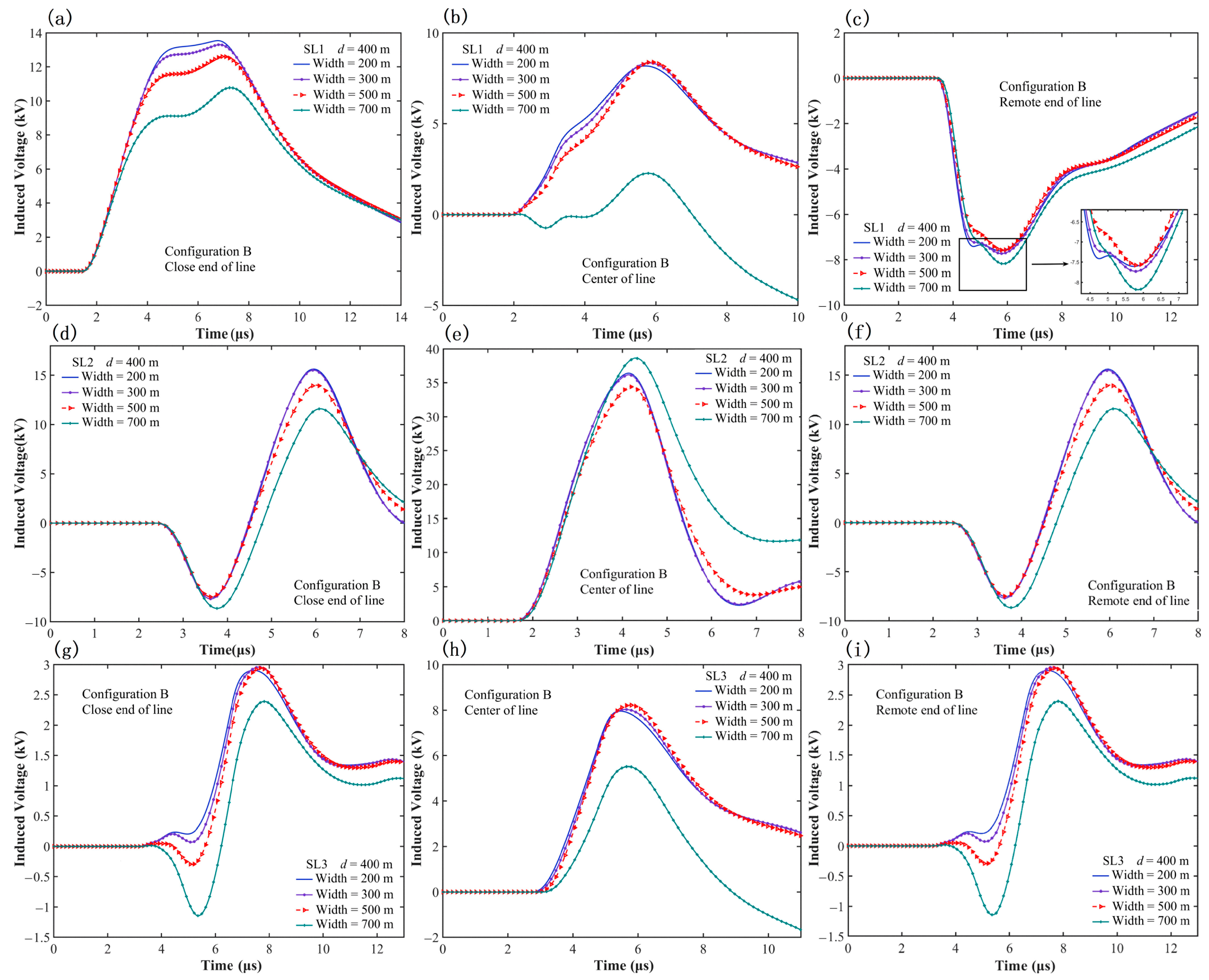
3.3. Impact of Gaussian-Shaped Mountain Width on LIVs

As analyzed in Section 3.2, we also compare the calculated LIVs for different Gaussian-shaped mountain widths. The mountain height is fixed to 250 m here, and the mountain widths are set to 200 m, 300 m, 500 m, and 700 m. Figure 9 presents the LIVs calculated along the distribution line, which is located 400 m horizontally from the mountain center, as shown in Figure 1.

For Configuration A, it can be seen from Figure 9a–c that the LIVs at the center and ends of the line decrease with increasing mountain width. For example, it can be found in

Table 5. Maximum LIVs of different mountain widths in Configuration A.

Strike Location	Width	Close End (kV)	Center (kV)	Remote End (kV)
SL1	200	14.21	6.13	16.07
	300	14.22	5.72	15.70
	500	13.46	4.39	13.92
	700	12.70	3.05	12.33
SL2	200	21.03	18.79	37.47
	300	20.79	19.15	37.79
	500	20.27	18.71	36.86
	700	22.44	18.62	35.33
SL3	200	14.03	8.66	16.94
	300	14.03	8.65	16.85
	500	13.92	8.49	16.26
	700	13.83	8.12	15.42

that the LIVs at the center of the line are reduced by approximately 6%, 27%, and 52% for 300 m, 500 m, and 700 m wide mountains than that of 200 m. Additionally, a larger mountain width leads to a longer peak arrival time. It can be explained that lightning EM waves propagate around the mountain due to terrain obstruction, which extends the propagation path for the case of SL1. In contrast to the case of SL1, as shown in Figure 9d–f for lightning strikes at SL2, the LIVs are significantly affected at the close end of the line only when the mountain width is relatively larger (500 m or 700 m). It is possible that the distance between the mountain base and the distribution line decreases as the mountain width increases. Observation points located closer to the mountain base are more sensitive to the reflection of lightning EM waves, whereas farther observation points are less affected, leading to less significant variation in LIVs at the remote end of the line, as shown in Figure 9e,f. However, the mountain’s shielding effect has a certain level of effect on LIVs when lightning strikes at SL3, as shown in Figure 9g–i, as the LIVs at both the line end and center decrease with increasing mountain width.

Figure 10 presents the results of LIVs along the distribution line for Configuration B and the maximum LIVs are presented in

Table 6. Maximum LIVs of different mountain widths in Configuration B.

Strike Location	Width	Close End (kV)	Center (kV)	Remote End (kV)
SL1	200	13.54	8.18	7.61
	300	13.31	8.34	7.73
	500	12.61	8.39	7.58
	700	10.78	2.27	8.18
SL2	200	15.68	36.39	15.68
	300	15.58	36.15	15.58
	500	14.07	34.3800	14.07
	700	11.71	38.62	11.71
SL3	200	2.95	7.96	2.95
	300	2.96	8.03	2.96
	500	2.99	8.22	2.99
	700	2.44	5.52	2.44

. Figure 10a–c shows the variations in LIVs when lightning strikes at SL1. It can be observed that as the mountain width increases to 500 m, the LIVs exhibit a significant attenuation, particularly at the close end and center of the line. This phenomenon is likely due to the close range between the mountain base and overhead distribution line for a larger mountain width, resulting in enhanced shielding of lightning EM fields by the mountain. For the case of SL2, Figure 10d,f exhibit identical results due to the symmetry of the terrain, it can be found that as mountain width increases to 500 m, it leads to an attenuation in LIVs at the ends of the line, whereas the induced voltage at center of the line increases when the mountain width reaches 700 m. For SL3, the calculated LIVs show that a significant decrease in the induced voltage at the center and ends of the line can be observed from Figure 10g–i when the mountain width reaches 700 m, this may be attributed to the attenuation effect introduced by the mountainous terrain [53]. Moreover, in the case of SL3 as shown in Figure 8g–i, taller mountains result in a delayed arrival time of the induced voltage peak. In contrast, variations in mountain width result in negligible differences in the peak arrival time. This can be explained by the propagation of the lightning EM waves, where the propagation path is primarily governed by the height of the mountain. As Hou et al. [54] discovered, the arrival time of EM waves is mainly dependent on the mountain height and is insensitive to the change in mountain width.

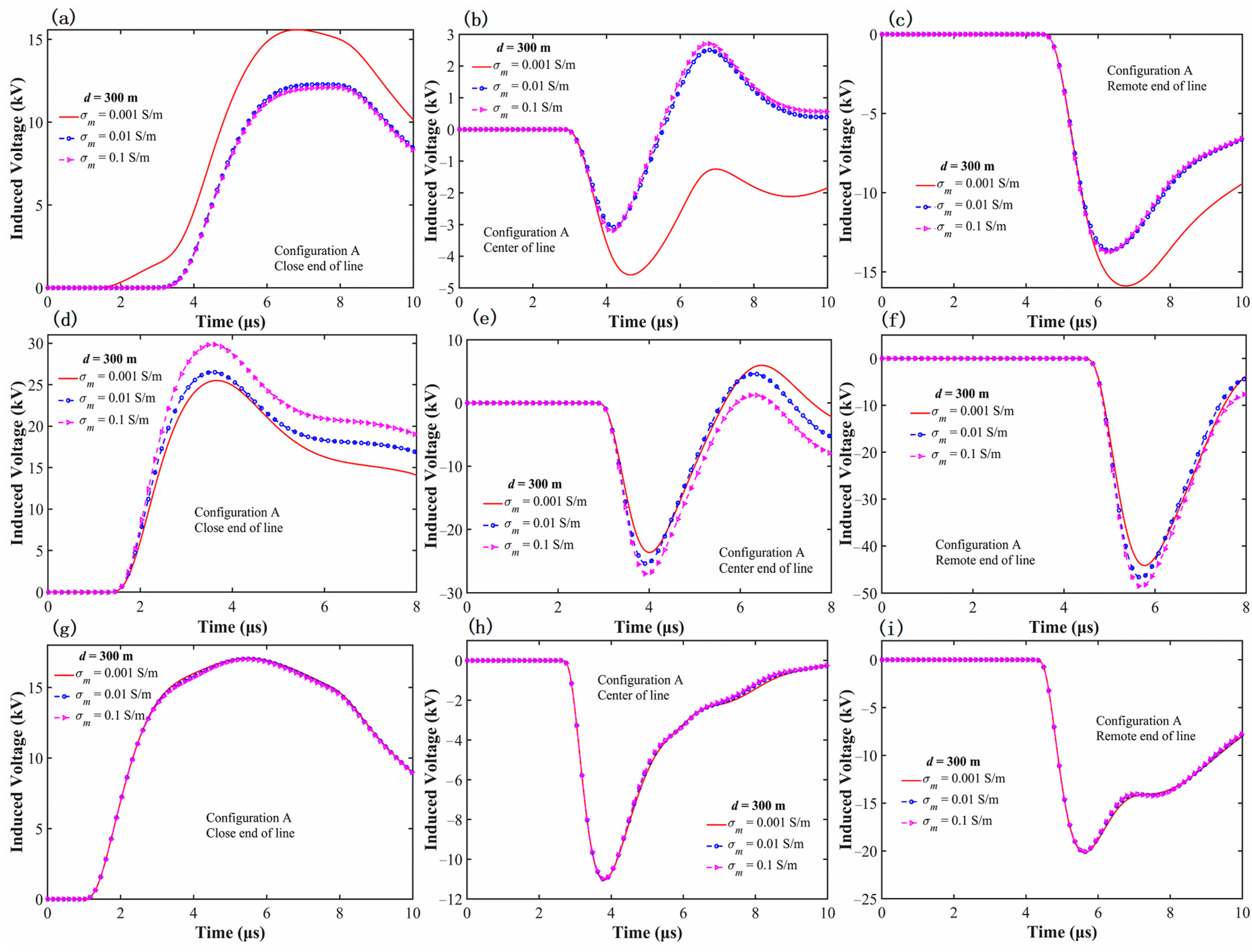
3.4. Impact of Mountain Conductivity on LIVs

The altitudinal variation in mountainous terrains results in distinct soil water content compared to flat ground, consequently changing the soil’s dielectric properties. In this section, we compare the calculated LIVs for different mountain conductivities σ_m ranging from 0.001 to 0.1 S/m considering different lightning strike locations. The mountain height and width are fixed to 250 m and 400 m here, and the ground soil conductivities σ_g are set to 0.001 S/m. Figure 11 and Figure 12 present the LIVs calculated along the distribution line, which is located 300 m horizontally from the mountain center, as shown in Figure 1.

Figure 11a–c shows the variations in LIVs along the distribution line when lightning strikes at SL1 in Configuration A. It can be found that a clear inverse correlation was observed between soil conductivity and LIVs. For example, at the close end of the line, the LIVs under 0.001 S/m soil conductivity exceeded those calculated at 0.01 S/m and 0.1 S/m by 32% and 33%, respectively. The observed nonlinear reduction in LIVs can be explained by enhanced attenuation of lightning-induced EM fields during propagation. Figure 11d–f show the variations in LIVs for lightning strikes at SL2, contrary to the results of SL1 where the LIVs increase with higher mountain conductivity. For SL3, as shown in Figure 11g–i, the effect of mountain conductivity is less pronounced. Figure 12 illustrates the LIVs along the distribution line in Configuration B. From Figure 12a–c, it can be observed that LIVs increase with lower mountain conductivity when lightning strikes at SL1. This effect is more significant on LIVs at the center of the distribution line, the LIV under 0.001 S/m mountain conductivity is increased by about 23% and 220%, compared to those with mountain conductivity of 0.01 S/m and 0.1 S/m. For lightning strikes at SL2, as demonstrated in Figure 12d–f, LIVs are more sensitive to variations in mountain conductivity at the center of the distribution line. As the results show in Figure 12e, the LIV under lower mountain conductivity of 0.001 S/m is increased by about 14% and 37% compared to those of 0.01 S/m and 0.1 S/m. The effect follows similar trends when lightning strikes at SL3, as shown in Figure 12g–i. However, LIVs exhibit a notable change at the center of the line only when mountain conductivity reaches up to 0.1 S/m.

4. Discussion

This study employs 3D-FDTD simulations to investigate LIV variations under lightning strikes at different locations on Gaussian-shaped mountains. Unlike previous numerical studies, the proposed Gaussian-shaped terrain better captures curved boundaries, which significantly influence lightning EM wave propagation. Previous studies [31] have confirmed that lightning striking a mountain can lead to an increase in LIVs on nearby distribution lines. In this study, the impact of mountains exhibits distinct patterns at different strike locations. The curved surface of the Gaussian-shaped mountain exhibits wave-focusing behavior, enhancing LIVs through stronger reflections when EM waves propagate along the surface while increasing shielding effects when waves propagate across the mountain. This effect is also influenced by the size of the mountain, as shown in the results, mountain height dominates LIVs more than width, with higher mountains amplifying both reflection and shielding effect. These results demonstrate that realistic mountain curvature must be considered in lightning protection design, as standard rectangular or cone-shaped models may underestimate LIV variations. Future work could extend this approach to complex terrain such as multi-peak terrains. From the results shown in Figure 11 and Figure 12, simulations reveal the necessity of distinguishing soil conductivity between mountain and ground due to their altitudinal positions and humidity. Future studies should pay more attention to the nonlinear correlation between soil conductivity and LIVs.

5. Conclusions

In this paper, LIVs along an overhead distribution line are calculated over a Gaussian-shaped mountain using the 3-D FDTD method. The height and width of the mountain, as well as the lightning strike locations, are considered to be the factors influencing the LIVs. The following conclusions are drawn from the results:

(1)

Comparative analysis reveals that the influence on LIVs for lightning strikes over complex mountainous terrain is pronounced. Different lightning strike locations correspond to different EM wave propagation paths. For lightning strikes at SL2, the presence of Gaussian-shaped mountainous terrain causes the enhancement in LIVs due to the reflection of EM waves between the mountain and the flat ground. However, the mountain obstructs the propagation of EM waves, which leads to attenuation in LIVs when lightning strikes at SL3.

(2)

For lightning strikes at SL1 and SL2, the presence of a Gaussian-shaped mountain leads to the enhancement of induced voltages, and this enhancement intensifies further as mountain height increases.

(3)

For lightning strikes at SL3, the Gaussian-shaped mountain is located between the lightning channel and the overhead distribution line. LIVs decrease compared to those of flat ground due to the shielding effect of the mountain, and this impact becomes more pronounced as the height increases.

(4)

In the case of a Gaussian-shaped mountain model, the influence of mountain width on the enhancement of LIVs is less significant than that of mountain height. Nonetheless, a sufficiently wide mountain can still result in a stronger EM shielding effect.

This paper investigates the impact of a single Gaussian-shaped mountain with finite soil conductivity on LIVs along a single overhead distribution line. The results demonstrate that the geometry of mountainous terrain significantly affects the LIVs for different lightning strike locations. However, in practical environments, distribution lines traverse multiple terrain features with varying electrical properties. Therefore, future work should extend the analysis to more complex terrain involving multiple mountains and varying soil dielectric properties. Additionally, two different placement configurations of single conductors are considered in this paper, as the coupling effects of multiple conductors also merit further investigation.

References

1. Rakov, V.A.; Rachidi, F. Overview of Recent Progress in Lightning Research and Lightning Protection. IEEE Trans. Electromagn. Compat. 2009, 51, 428–442. [Google Scholar] [CrossRef]
2. Ahmad, N.I.; Ab-Kadir, M.Z.A.; Izadi, M.; Azis, N.; Radzi, M.A.M.; Zaini, N.H.; Nasir, M.S.M. Lightning Protection on Photovoltaic Systems: A Review on Current and Recommended Practices. Renew. Sustain. Energy Rev. 2018, 82, 1611–1619. [Google Scholar] [CrossRef]
3. Chowdhuri, P. Parameters of Lightning Strokes and Their Effects on Power Systems. In Proceedings of the 2001 IEEE/PES Transmission and Distribution Conference and Exposition: Developing New Perspectives, Atlanta, GA, USA, 2 November 2001; pp. 1047–1051. [Google Scholar] [CrossRef]
4. Le Vine, D.M.; Meneghini, R. Electromagnetic Fields Radiated from a Lightning Return Stroke: Application of an Exact Solution to Maxwell’s Equations. J. Geophys. Res. Ocean. 1978, 83, 2377–2384. [Google Scholar] [CrossRef]
5. Bakar, A.; Abidin, A.Z.; Illias, H.; Mokhlis, H.; Halim, S.A.; Hassan, N.H.N.; Tan, C.K. Determination of the Striking Distance of a Lightning Rod Using Finite Element Analysis. Turk. J. Electr. Eng. Comput. Sci. 2016, 24, 4083–4097. [Google Scholar] [CrossRef]
6. Napolitano, F.; Borghetti, A.; Nucci, C.A.; Rachidi, F.; Paolone, M. Use of the Full-Wave Finite Element Method for the Numerical Electromagnetic Analysis of LEMP and Its Coupling to Overhead Lines. Electr. Power Syst. Res. 2013, 94, 24–29. [Google Scholar] [CrossRef]
7. Baba, Y.; Rakov, V.A. Applications of the FDTD Method to Lightning Electromagnetic Pulse and Surge Simulations. IEEE Trans. Electromagn. Compat. 2014, 56, 1506–1521. [Google Scholar] [CrossRef]
8. Li, D.; Zhang, Q.; Wang, Z.; Liu, T. Computation of Lightning Horizontal Field Over the Two-Dimensional Rough Ground by Using the Three-Dimensional FDTD. IEEE Trans. Electromagn. Compat. 2014, 56, 143–148. [Google Scholar] [CrossRef]
9. Hu, W.; Cummer, S.A. An FDTD Model for Low and High-Altitude Lightning-Generated EM Fields. IEEE Antennas Propag. Mag. 2006, 54, 1513–1522. [Google Scholar] [CrossRef]
10. Tatematsu, A.; Rachidi, F.; Rubinstein, M. Analysis of Electromagnetic Fields Inside a Reinforced Concrete Building with Layered Reinforcing Bar Due to Direct and Indirect Lightning Strikes Using the FDTD Method. IEEE Trans. Electromagn. Compat. 2015, 57, 405–417. [Google Scholar] [CrossRef]
11. La Fata, A.; Nicora, M.; Mestriner, D.; Aramini, R.; Procopio, R.; Brignone, M.; Delfino, F. Lightning Electromagnetic Fields Computation: A Review of the Available Approaches. Energies 2023, 16, 2436. [Google Scholar] [CrossRef]
12. Rachidi, F. A Review of Field-to-Transmission Line Coupling Models with Special Emphasis to Lightning-Induced Voltages on Overhead Lines. IEEE Trans. Electromagn. Compat. 2012, 54, 898–911. [Google Scholar] [CrossRef]
13. Taylor, C.D.; Satterwhite, R.S.; Harrison, C.W. The Response of Terminated Two-Wire Transmission Line Excited by Nonuniform Electromagnetic Field. IEEE Trans. Antennas Propag. 1965, 13, 987–989. [Google Scholar] [CrossRef]
14. Rachidi, F. Formulation of Field-to-Transmission Line Coupling Equations in Terms of Magnetic Excitation Field. IEEE Trans. Electromagn. Compat. 1993, 35, 404–407. [Google Scholar] [CrossRef]
15. Agrawal, A.K.; Price, H.J.; Gurbaxani, S.H. Transient Response of Multiconductor Transmission Lines Excited by a Nonuniform Electromagnetic Field. IEEE Trans. Electromagn. Compat. 1980, EMC-22, 119–129. [Google Scholar] [CrossRef]
16. Pokharel, R.K.; Ishii, M.; Baba, Y. Numerical Electromagnetic Analysis of Lightning-Induced Voltage over Ground of Finite Conductivity. IEEE Trans. Electromagn. Compat. 2003, 45, 651–656. [Google Scholar] [CrossRef]
17. Liu, Y.; Jiang, Y.; Gao, Q.; Li, X.; Yang, G.; Zhang, Q.; Tang, B. Influences of Soil Water Content and Porosity on Lightning Electromagnetic Fields and Lightning-Induced Voltages on Overhead Lines. Front. Environ. Sci. 2022, 10, 946551. [Google Scholar] [CrossRef]
18. Ishii, T.; Oguchi, S.; Sakamoto, Y.; Okabe, S. A Field Study of Lightning Overvoltages in Low-Voltage Distribution Lines. Electr. Eng. Jpn. 2013, 183, 12–21. [Google Scholar] [CrossRef]
19. Hossain, M.K.; Tasnim, L. Analysis of the Impact of Ground Conductivity, Source Current Speed, and Source Current Rise Time on Peak Induced Voltage on Overhead Conductors. Discov. Electron. 2025, 2, 3. [Google Scholar] [CrossRef]
20. Sun, Q.; Zhong, X.; Liu, J.; Wang, F.; Chen, S.; Zhong, L.; Bian, X. Three-Dimensional Modeling on Lightning Induced Overvoltage for Photovoltaic Arrays Installed on Mountain. J. Clean. Prod. 2021, 288, 125664. [Google Scholar] [CrossRef]
21. Nematollahi, A.F.; Vahidi, B.; Mousavi, E.S.A. The Indirect-Lightning Performance of Overhead Distribution Line Considering the Mixed Ocean–Land Propagation Path. IEEE Trans. Electromagn. Compat. 2023, 66, 1137–1145. [Google Scholar] [CrossRef]
22. Li, D.; Azadifar, M.; Rachidi, F.; Rubinstein, M.; Paolone, M. On Lightning Electromagnetic Field Propagation Along an Irregular Terrain. IEEE Trans. Electromagn. Compat. 2015, 58, 161–171. [Google Scholar] [CrossRef]
23. Mestriner, D.; Marchesoni, F.; Procopio, R.; Brignone, M. Attenuation of Lightning-Induced Effects on Overhead Distribution Systems in Urban Areas. Appl. Sci. 2022, 12, 7632. [Google Scholar] [CrossRef]
24. Nicora, M.; Mestriner, D.; Brignone, M.; Procopio, R.; Fiori, E.; Piantini, A.; Rachidi, F. Estimation of the Lightning Performance of Overhead Lines Accounting for Different Types of Strokes and Multiple Strike Points. IEEE Trans. Electromagn. Compat. 2021, 63, 2015–2023. [Google Scholar] [CrossRef]
25. Natsui, M.; Ametani, A.; Mahseredjian, J.; Sekioka, S.; Yamamoto, K. 3-D FDTD Analysis of Lightning-Induced Voltages in Distribution Lines Due to Inclined Lightning. IEEE Trans. Electromagn. Compat. 2020, 63, 189–197. [Google Scholar] [CrossRef]
26. Petrarca, C.; Balato, M.; Verolino, L.; Andreotti, A.; Assante, D. Computation of Electric and Magnetic Fields Generated by Cloud-to-Cloud Lightning Channels. Energies 2023, 16, 4524. [Google Scholar] [CrossRef]
27. Rizk, M.E.; Abulanwar, S.; Ghanem, A.; Lehtonen, M. Computation of Lightning-Induced Voltages Considering Ground Impedance of Multi-Conductor Line for Lossy Dispersive Soil. IEEE Trans. Power Del. 2021, 37, 2464–2473. [Google Scholar] [CrossRef]
28. Zhang, J.; Zhang, Q.; Hou, W.; Zhang, L.; Zhou, F.; Ma, Y.; Ma, Y. Evaluation of the Lightning-Induced Voltages of Multiconductor Lines for Striking Cone-Shaped Mountain. IEEE Trans. Electromagn. Compat. 2018, 61, 1534–1542. [Google Scholar] [CrossRef]
29. Soto, E.; Perez, E.; Herrera, J. Electromagnetic Field Due to Lightning Striking on Top of a Cone-Shaped Mountain Using the FDTD. IEEE Trans. Electromagn. Compat. 2014, 56, 1112–1120. [Google Scholar] [CrossRef]
30. Soto, E.; Pérez, E. Lightning-Induced Voltages on Overhead Lines over Irregular Terrains. Electr. Power Syst. Res. 2019, 176, 105941. [Google Scholar] [CrossRef]
31. Zhang, J.; Zhang, Q.; Zhou, F.; Ma, Y.; Pan, H.; Hou, W. Computation of Lightning-Induced Voltages for Striking Oblique Cone-Shaped Mountain by 3-D FDTD Method. IEEE Trans. Electromagn. Compat. 2019, 61, 1543–1551. [Google Scholar] [CrossRef]
32. Arzag, K.; Azzouz, Z.E.; Baba, Y.; Ghemri, B. 3-D FDTD Computation of Electromagnetic Fields Associated with Lightning Strikes to a Tower Climbed on a Trapezoidal Mountain. IEEE Trans. Electromagn. Compat. 2019, 61, 606–616. [Google Scholar] [CrossRef]
33. Zaini, N.H.; Ab Kadir, M.Z.A.; Mohd Radzi, M.A.; Izadi, M.; Azis, N.; Ahmad, N.I.; Nasir, M.S.M. Lightning Surge Analysis on a Large Scale Grid-Connected Solar Photovoltaic System. Energies 2017, 10, 2149. [Google Scholar] [CrossRef]
34. Ahmad, N.I.; Ali, Z.; Ab Kadir, M.Z.A.; Osman, M.; Zaini, N.H.; Roslan, M.H. Impacts of Lightning-Induced Overvoltage on a Hybrid Solar PV–Battery Energy Storage System. Appl. Sci. 2021, 11, 3633. [Google Scholar] [CrossRef]
35. Sun, Q.; Zhong, X.; Zhong, L.; Wang, F.; Liu, J.; Chen, S.; Yang, T. Investigation on Induced Voltage of Photovoltaic System on Complex Terrain. Electr. Power Syst. Res. 2021, 201, 107549. [Google Scholar] [CrossRef]
36. Willatzen, M. Electromagnetic-Wave Propagation along Curved Surfaces. Phys. Rev. A—At. Mol. Opt. Phys. 2009, 80, 043805. [Google Scholar] [CrossRef]
37. Donohue, J.D.; Kuttler, J.R. Propagation Modeling over Terrain Using the Parabolic Wave Equation. IEEE Trans. Antennas Propag. 2000, 48, 260–277. [Google Scholar] [CrossRef]
38. Yu, J.; Gu, S.; Liu, J.; Liu, H. Indirect lightning performance of 10-kV overhead distribution lines. Front. Energy Res. 2024, 12, 1367183. [Google Scholar] [CrossRef]
39. Teixeira, F.L.; Sarris, C.; Zhang, Y.; Na, D.Y.; Berenger, J.P.; Su, Y.; Okoniewski, M.; Chew, W.C.; Backman, V.; Simpson, J.J. Finite-Difference Time-Domain Methods. Nat. Rev. Methods Primers 2023, 3, 75. [Google Scholar] [CrossRef]
40. Mohamed, E.; Souli, A.; Beladel, A.; Khaleel, M. Simulation and Analysis of Lightning Strikes in Electrical Systems by MATLAB/SIMULINK and ATP/EMTP. ITEGAM-JETIA 2024, 10, 142–150. [Google Scholar] [CrossRef]
41. Yang, B.; Zhou, B.H.; Gao, C.; Shi, L.H.; Chen, B.; Chen, H.L. Using a two-step finite-difference time-domain method to analyze lightning-induced voltages on transmission lines. IEEE Trans. Electromagn. Compat. 2011, 53, 256–260. [Google Scholar] [CrossRef]
42. Mur, G. Absorbing Boundary Conditions for the Finite-Difference Approximation of the Time-Domain Electromagnetic-Field Equations. IEEE Trans. Electromagn. Compat. 1981, EMC-23, 377–382. [Google Scholar] [CrossRef]
43. Yu, W.; Mittra, R. A Conformal Finite Difference Time Domain Technique for Modeling Curved Dielectric Surfaces. IEEE Microw. Wirel. Compon. Lett. 2001, 11, 25–27. [Google Scholar] [CrossRef]
44. Yu, W.; Mittra, R. A Conformal FDTD Algorithm for Modeling Perfectly Conducting Objects with Curve-Shaped Surfaces and Edges. Microw. Opt. Technol. Lett. 2000, 27, 136–138. [Google Scholar] [CrossRef]
45. Heidler, F.; Cvetic, J.M.; Stanic, B.V. Calculation of Lightning Current Parameters. IEEE Trans. Power Deliv. 1999, 14, 399–404. [Google Scholar] [CrossRef]
46. Nucci, C.A.; Rachidi, F.; Ianoz, M.V.; Mazzetti, C. Lightning-Induced Voltages on Overhead Lines. IEEE Trans. Electromagn. Compat. 1993, 35, 75–86. [Google Scholar] [CrossRef]
47. Nucci, C.A.; Mazzetti, C.; Rachidi, F.; Ianoz, M.V. On Lightning Return Stroke Models for LEMP Calculations. In Proceedings of the 19th International Conference on Lightning Protection, Graz, Austria, 25–29 April 1988; pp. 463–469. [Google Scholar]
48. Baba, Y.; Rakov, V.A. On the Transmission Line Model for Lightning Return Stroke Representation. Geophys. Res. Lett. 2003, 30, 2294. [Google Scholar] [CrossRef]
49. Thottappillil, R.; Uman, M.A. Comparison of Lightning Return-Stroke Models. J. Geophys. Res. Atmos. 1993, 98, 22903–22914. [Google Scholar] [CrossRef]
50. Alves, A.F.S.; Araújo, M.A. Survey on Analytical and Numerical Methods for Lightning-Induced Voltages Calculations. Electr. Eng. 2024, 106, 905–916. [Google Scholar] [CrossRef]
51. Li, D.; Azadifar, M.; Rachidi, F.; Rubinstein, M.; Diendorfer, G.; Sheshyekani, K.; Zhang, Q.; Wang, Z. Analysis of Lightning Electromagnetic Field Propagation in Mountainous Terrain and Its Effects on ToA-Based Lightning Location Systems. J. Geophys. Res. Atmos. 2016, 121, 895–911. [Google Scholar] [CrossRef]
52. Hou, W.; Zhang, Q.; Wang, L.; Zhang, J. Effect of Striking a Cone-Shaped Mountain Top on the Far Lightning-Radiated Electromagnetic Field. IEEE Trans. Electromagn. Compat. 2019, 61, 1147–1156. [Google Scholar] [CrossRef]
53. Su, Z.; Lyu, W.; Chen, L.; Wu, S. Shielding Effect of Surrounding Buildings on the Lightning-Generated Vertical Electric Field at the Top of a Tall Building. IEEE Trans. Electromagn. Compat. 2018, 61, 174–182. [Google Scholar] [CrossRef]
54. Hou, W.; Azadifar, M.; Rubinstein, M.; Rachidi, F.; Zhang, Q. On the Propagation of Lightning-Radiated Electromagnetic Fields Across a Mountain. IEEE Trans. Electromagn. Compat. 2020, 62, 2137–2147. [Google Scholar] [CrossRef]
55. Peng, X.; Wang, L.; Zhang, J.; Chen, J.; Dai, B. The Field Shielding Effect of Mountain on the Lightning Electromagnetic Field. J. Electromagn. Anal. Appl. 2020, 12, 15–28. [Google Scholar] [CrossRef]
Figure 1. Geometry of Gaussian-shaped terrain developed in our 3-D FDTD model. Side view and top view for two different line configurations: (a) Configuration A and (b) Configuration B.
Applsci 15 06428 g001
Figure 2. 3-D illustration of the locally conformal FDTD technique is adopted to modify the dielectric parameters in a Yee cell.
Applsci 15 06428 g002
Figure 3. Channel-based current waveform of a sum of two Heidler in time domain.
Applsci 15 06428 g003
Figure 4. Comparison of results obtained from Zhang et al. [31] with that from our 3-D FDTD model adopted in this study for calculating the LIVs when lightning strikes a cone-shaped mountain with different inline angles.
Applsci 15 06428 g004
Figure 5. Comparison among the lightning-induced voltages for Configuration A over different terrains, including flat ground, Gaussian-shaped, and cone-shaped mountains. LIVs of line close end, center, and remote end when lightning strikes at (ac) SL1, (df) SL2, (gi) SL3, respectively.
Applsci 15 06428 g005
Figure 6. Comparison among the lightning-induced voltages for Configuration B over different terrains, including flat ground, Gaussian-shaped, and cone-shaped mountains. LIVs of line close end, center, and remote end when lightning strikes at (ac) SL1, (df) SL2, (gi) SL3, respectively.
Applsci 15 06428 g006
Figure 7. Comparison among the lightning-induced voltages for Configuration A over Gaussian-shaped mountain, considering different mountain heights ranging from 200 m to 400 m. LIVs of line close end, center, and remote end when lightning strikes at (ac) SL1, (df) SL2, (gi) SL3, respectively.
Applsci 15 06428 g007
Figure 8. Comparison among the lightning-induced voltages for Configuration B over Gaussian-shaped mountain, considering different mountain heights ranging from 200 m to 400 m. LIVs of line close end, center, and remote end when lightning strikes at (ac) SL1, (df) SL2, (gi) SL3, respectively.
Applsci 15 06428 g008
Figure 9. Comparison among the lightning-induced voltages for Configuration A over Gaussian-shaped mountain, considering different mountain widths ranging from 200 m to 700 m. LIVs of line close end, center, and remote end when lightning strikes at (ac) SL1, (df) SL2, (gi) SL3, respectively.
Applsci 15 06428 g009
Figure 10. Comparison among the lightning-induced voltages for Configuration B over Gaussian-shaped mountain, considering different mountain widths ranging from 200 m to 700 m. LIVs of line close end, center, and remote end when lightning strikes at (ac) SL1, (df) SL2, (gi) SL3, respectively.
Applsci 15 06428 g010
Figure 11. Comparison among the lightning-induced voltages for Configuration A over Gaussian-shaped mountain, considering different σm ranging from 0.001 to 0.1 S/m. LIVs of line close end, center, and remote end when lightning strikes at (ac) SL1, (df) SL2, (gi) SL3, respectively.
Applsci 15 06428 g011
Figure 12. Comparison among the lightning-induced voltages for Configuration B over Gaussian-shaped mountain, considering different σm ranging from 0.001 to 0.1 S/m. LIVs of line close end, center, and remote end when lightning strikes at (ac) SL1, (df) SL2, (gi) SL3, respectively.
Applsci 15 06428 g012