Article

A Machine Learning Approach for Predicting Particle Spatial, Velocity, and Temperature Distributions in Cold Spray Additive Manufacturing

Department of Mechanical and Industrial Engineering, University of Toronto, 5 King’s College Rd., Toronto, ON M5S 3G8, Canada
*
Author to whom correspondence should be addressed.
Appl. Sci. 2025, 15(12), 6418; https://doi.org/10.3390/app15126418
Submission received: 26 April 2025 / Revised: 1 June 2025 / Accepted: 3 June 2025 / Published: 7 June 2025

Abstract

Masked cold spray additive manufacturing (CSAM) is investigated for fabricating nickel-based electrodes with pyramidal pin-fins that enlarge the active area for the hydrogen-evolution reaction (HER). To bypass the high cost of purely CFD-driven optimization, we construct a two-stage machine learning (ML) framework trained on 48 high-fidelity CFD simulations. Stage 1 applies sampling and a K-nearest-neighbor kernel-density-estimation algorithm that predicts the spatial distribution of impacting particles and re-allocates weights in regions of under-estimation. Stage 2 combines sampling, interpolation and symbolic regression to extract key features, then uses a weighted random forest model to forecast particle velocity and temperature upon impact. The ML predictions closely match CFD outputs while reducing computation time by orders of magnitude, demonstrating that ML-CFD integration can accelerate CSAM process design. Although developed for a masked setup, the framework generalizes readily to unmasked cold spray configurations.

1. Introduction

Cold spray is an advanced additive manufacturing and repair process that utilizes high-pressure carrier gases, such as nitrogen or helium, to accelerate solid micron-sized particles to high velocities through a converging-diverging nozzle. This technique enables rapid material deposition without melting, relying solely on the particles’ kinetic energy for adhesion [1,2,3,4,5]. Upon impact with the substrate, the particles undergo severe plastic deformation, forming strong bonds with the surface. This low-temperature process avoids the thermal damage typically associated with high-temperature methods, preserving the original properties of both the feedstock and the substrate [3,6]. As a result, cold spray is particularly advantageous for industrial applications requiring high-quality, thermally sensitive material deposition.
In high-pressure cold spray systems, operating pressures range from 1 to 5 MPa, with gas temperatures reaching up to 1100 °C—remaining below the melting point of the particles [7]. Under these conditions, particles are accelerated to velocities typically between 500 and 1000 m/s. A crucial parameter in the deposition process is the standoff distance (SOD), which defines the gap between the nozzle exit and the substrate [2]. Along with SOD, factors such as nozzle geometry, operating conditions, particle type and size, and carrier gas properties play a significant role in determining particle velocity and temperature upon impact, deposition efficiency (DE), and coating quality [8]. The ability to finely control these parameters while minimizing thermal effects makes cold spray a vital technique in modern manufacturing and repair applications.
Recent studies demonstrate the potential of hydrogen evolution reactions (HER) for renewable energy. However, commercial-scale hydrogen production is still obscured by the challenges of producing stable and cost-effective electrocatalysts [9]. More specifically, while noble-metal-based catalysts demonstrate excellent catalytic performance, their high cost and limited availability hinder commercial applications [9]. Nickel, as a non-noble metal, provides a promising alternative, though its catalytic performance is inherently lower. To address this, increasing the electrode’s surface area through surface modification has been a key focus [10]. Aghasibeig et al. [11] demonstrated that cold-sprayed nickel samples achieved superior electrocatalytic activity compared to smooth nickel electrodes. This enhancement was attributed to increased active surface area and improved surface roughness, which enhanced the efficiency of the electrolysis process. The creation of fin geometries using a mask (or a wire mesh) positioned between the nozzle exit and the substrate further amplifies these effects. By guiding particle flow through its openings, the mask facilitates the formation of pyramidal pin fins on the substrate surface. These structures not only increase the active surface area considerably but also significantly enhance surface roughness, improving catalytic performance by providing more active sites for electrochemical reactions. Studies using masked High-Velocity Oxy-Fuel (HVOF) spraying [12], masked atmospheric plasma spraying, and masked suspension plasma spraying [10] confirmed that electrodes coated with a mask exhibited greater electrocatalytic activity, primarily due to the enhanced roughness levels achieved during deposition.
In our previous study [13], we employed Computational Fluid Dynamics (CFD) to investigate a three-dimensional high-pressure masked cold spray nozzle, using nickel powder as the injection feedstock. The simulations were based on the PCS 800 cold spray system (Plasma Giken, Yoriimachi, Japan). The parametric study examined four masks with varying wire thicknesses and opening sizes, positioned at 4 mm increments from the nozzle exit. Substrates were placed at SODs of 10 mm and 20 mm. To evaluate the effect of gas inlet conditions, simulations were performed under two nozzle inlet settings: 2 MPa and 400 °C, and 4 MPa and 800 °C. Particle behavior was effectively modeled using a two-way coupled Eulerian–Lagrangian approach. The findings revealed that nozzle inlet conditions had the greatest impact on particle velocity, temperature, and powder deposition. Under high-pressure conditions (4 MPa), DE exceeded 99.9% across all the test cases, ensuring nearly complete particle adherence to the substrate. In contrast, at medium pressure (2 MPa), DE increased linearly with mask SOD, attributed to the rise in particle velocity upon impact.
While CFD and modern experimental equipment effectively capture particle in-flight behavior, predicting particle velocity and temperature upon impact under various conditions requires numerous simulations and experiments due to the many parameters involved in the process. A comprehensive exploration of these parameters, both individually and collectively, is challenging owing to the high computational cost, long processing time of simulations, and the expense and extended duration of experimental measurements. To address these limitations, machine learning (ML) provides a promising alternative by leveraging data-driven approaches to identify relationships between parameters like inlet pressure, substrate SOD, mask SOD, mask properties, and deposition characteristics.
ML has been utilized to predict particle velocity in plasma and cold spray processes. Bobzin et al. [14] employed Residual Neural Network (ResNN) and Support Vector Regression (SVR) approaches, and used CFD simulations of the plasma spray process to generate training data. Despite the stochastic nature of the process, both models achieved high accuracy in predicting average particle velocity, with R2 values of 97% and 99%, though their Mean Absolute Percentage Error (MAPE) remained around 20% on unseen data. For cold spray, Canales et al. [15] applied ML classification algorithms to distinguish between deposited and not-deposited particles based on kinetic and thermal energies obtained from CFD simulations, achieving classification accuracies of 98–99% for aluminum and copper particles. Moreover, Eberle et al. [16] applied SVR and neural network (NN) to predict particle velocity distribution and deposition efficiency in the cold spraying of titanium using experimental data. While the models accurately predicted the average particle velocity, they struggled with single-particle velocity due to stochastic effects.
This study aims to develop a stacked ML model for the rapid and accurate prediction of particle spatial, velocity, and temperature distributions upon impact on a substrate in masked cold spray additive manufacturing. This ML framework comprises two primary models. The first model predicts the spatial distribution of particles on the substrate. The output of this model then serves as the basis for the second model, which forecasts the particle velocity and temperature distributions upon impact. Unlike classical cold spray deposition on a flat substrate, masked cold spray introduces additional complexity, requiring advanced modeling to capture the intricate interactions between particles, masks, and the substrate. This ML framework is trained on a dataset of 48 CFD simulations from our previous study [13], with multiple strategies employed to enhance its predictive capabilities. This approach significantly reduces computational costs and processing time while offering strong adaptability to dynamic boundary conditions, making it a scalable and efficient solution for optimizing the cold spray process [17] and enhancing the electrocatalytic performance of nickel-based electrodes. A detailed discussion of the methodology and training of the ML model is provided in the following section, while the results of the chosen ML models are presented in the results section.

2. Methodology

The dataset used in this study is derived from 3D CFD simulations of the masked cold spray process [13], where nickel powder serves as the injection feedstock. Due to the inherent flow and geometric symmetries of the process, a quarter-symmetric model was employed, as illustrated in Figure 1. As shown in Figure 1 and discussed in the introduction, our previous study conducted 48 simulations, systematically varying mask types, substrate SODs, mask SODs, and nozzle inlet conditions to assess their impact on particle spatial, velocity, and temperature distributions at the substrate [13]. Figure 1 also presents a representative CFD-simulated map of particle impact velocity on the substrate under medium-pressure inlet conditions [13].
The overall methodology consists of three key components: sampling, the first model, and the second model. The entire workflow is illustrated in Figure 2. Initially, the sampling phase selects representative data points that serve as the foundation for subsequent analysis. Next, the first model employs a KNN-based KDE prediction method (KNN and KDE stand for K-nearest neighbors and kernel density estimation, respectively) in conjunction with a projection algorithm to predict the spatial distribution of particles on the substrate. The input parameters for the first model include mask properties, substrate SODs, mask SODs, nozzle inlet conditions, and particle size distribution (ranging from 17 μm to 77 μm with a mean diameter of 48 μm—commonly used in cold spray processes—and modeled in CFD simulations using a Rosin–Rammler distribution). A summary of the input features for the first ML model is provided below.
Inputs1 = [particle diameter, mask properties (wire diameter, opening size, open area), mask SOD, substrate SOD, inlet condition (inlet pressure and inlet temperature)]
The outputs are the spatial positions of particles on the substrate, represented by the y- and z-coordinates. In other words, the y- and z-coordinates indicate the horizontal and vertical positions of the particles on the substrate surface (see Figure 1).
Outputs1 = [y-positions of particles, z-positions of particles]
Specifically, this model employs the KNN-KDE approach to generate preliminary predictions while incorporating physical priors to identify invalid cases (such as points within the dead zone—regions behind the wires where particle deposition is almost zero (e.g., around point (1,1) in the sample CFD result shown in Figure 1)) and under-estimated regions. Subsequently, weight assignment and local reallocation strategies are applied to remap these invalid predictions to physically plausible locations.
Finally, the second model predicts the particle velocity and temperature distributions upon impact on a substrate. The input parameters for the second ML model include mask properties, substrate SODs, mask SODs, nozzle inlet conditions, particle size distribution, and the spatial positions of particles on the substrate (the prediction of the first model (y- and z-coordinates)). A summary of the input features for the second ML model is provided below.
Inputs2 = [y-positions of particles, z-positions of particles, particle diameter, mask properties (wire diameter, opening size, open area), mask SOD, substrate SOD, inlet condition (inlet pressure and inlet temperature)]
The outputs are the velocity and temperature of each particle upon impact on the substrate. The output features are provided below
Outputs2 = [u, v, w, T]
where u, v, and w represent the particle velocity components upon impact along the x-, y-, and z-directions, respectively, and T denotes the particle temperature on the substrate.
The second model is composed of three sequential steps: interpolation is first used to fill gaps in the data; next, mathematical transformations are applied to refine the original features—for instance, by employing additive operations to generate new features that better capture the underlying data patterns; and finally, model optimization is performed via the fine-tuning of parameters to further enhance predictive accuracy. The following sections provide a detailed explanation of each step shown in Figure 2.

2.1. Sampling

Typically, each CFD simulation contains hundreds of thousands of data points. In our previous study [13], a single simulation included nearly a million data points representing particles trapped on the substrate, making it impractical to use the raw simulation results directly for machine learning due to high computational demands. To overcome this challenge, we propose a sampling method that combines feature stratification with greedy sampling to extract representative subsets from the large dataset. Importantly, the data obtained through this sampling approach is used in both models, ensuring that each model benefits from a consistent and representative dataset while significantly reducing computational resource consumption.
Firstly, the CFD results indicate that axial powder injection and higher gas velocity along the jet centerline cause most particles to remain near the centerline (see the particle distribution in Figure 1, where the point (y = 0, z = 0) represents the jet centerline), gaining significant thrust and momentum in this region. As a result, random sampling could disproportionately select points from the central region (i.e., near the jet centerline), leading to oversampling there and undersampling in other regions. To mitigate this, stratified sampling based on the particles’ y- and z-coordinates is adopted to ensure balanced representation across different regions. Specifically, particles are initially sorted in ascending order based on their y-coordinate values (feature y).
y 1 , y 2 , y 3 , y N y N 1 < y N
To ensure an even distribution of particles within each interval in terms of horizontal coordinate, a quantile-based partitioning method is employed.
q k = k b y k = 1 , 2 , , b y 1
where q k is the k-th quantile of y and b y is the number of intervals. Based on the quantiles, the particles sorted by their y-coordinates are divided into b y intervals. Each interval contains an approximately equal number of particles, ensuring uniform distribution within each y-coordinate range. This partitioning ensures that the stratified sampling captures the characteristics of the data across the entire y-coordinate spectrum without overrepresenting or underrepresenting any specific region.
a 0 , a 1 , a 1 , a 2 , [ a b y 1 , a b y ] a 0 = min y ,   a b y = m a x ( y )
For each k   = 1 , 2 , , b y 1 , a k serves as the boundary that separates adjacent bins for feature y. Then, the bin number for each particle is determined based on the interval in which its value falls (Equation (8)). By assigning a bin number corresponding to its respective y-coordinate interval, each particle is effectively categorized with respect to the y-coordinate.
b i n I n d e x y = 0 ,                   i f   y a 0 , a 1   1 ,                   i f   y a 0 , a 1                                    
Similarly, each particle can undergo the same process to obtain an index based on stratification by its z-coordinate. By combining the indices derived from both the y- and z-coordinates, a multidimensional stratification is achieved (Equation (9)). This approach ensures that particles within the same bin are located in similar positions, while particles from different bins occupy distinct positions. This multidimensional stratification enhances the representativeness of the sampled data by capturing variations across both coordinates.
s t r a t u m x = ( b i n I n d e x y , b i n I n d e x z )
After completing the stratification based on y- and z-coordinates, all the non-empty layer labels are extracted to form a layer set (Equation (10)). This layer set represents the combined stratification indices of particles across the y- and z-coordinate dimensions. Each label in the set corresponds to a unique bin containing particles.
L = { l 1 , l 2 , , l N }
where l i stands for a specific multidimensional feature combination region, and N is the total number of layers here. If the global target sample size is {SampleSize}, it is first distributed across all the layers as evenly as possible to ensure uniform allocation (Equation (11)).
b a s e l i = S a m p l e S i z e N
If {SampleSize} cannot be evenly divided by the total number of layers, the remaining samples will be randomly allocated to a subset of the layers.
Next, for each labeled layer l i , sampling is performed from the particles within that layer. If the number of particles in the current layer is less than or equal to the assigned sample size, all the particles in the layer are directly selected. However, if the number of particles exceeds the assigned sample size, a greedy algorithm is applied to determine the samples. A schematic of the stratified and greedy sampling process is shown in Figure 3.
The purpose of the greedy algorithm is to select data points from the layer that are as diverse or dispersed as possible within the feature space. The algorithm generally follows three steps: (1) randomly select a seed point and add it to the sample set; (2) standardize all features to eliminate scale differences; (3) iteratively choose the candidate point that maximizes its minimum Euclidean distance from the current sample set.
As mentioned, first, a point is randomly selected as the seed point x and added to the sample set C . Then, in each iteration, the algorithm evaluates all the unselected candidate points. Specifically, for each candidate, it computes its Euclidean distance from the current sample set C ; that is, it calculates the distances between the candidate and every point in the sample set and takes the minimum of these distances (i.e., the distance from the candidate to its nearest sample) (Equations (12) and (13)). This minimum value serves as the criterion to assess the candidate’s remoteness from the existing samples. The algorithm then selects the candidate with the largest “minimum distance” to be added to the sample set, ensuring that the newly added point is as far as possible from the current samples and thereby guaranteeing that all types of data have an opportunity to be sampled. All the features are standardized before the calculation to avoid errors caused by significant differences in scale between features (Equation (14)).
x next = a r g m a x x S l i \ C min c C x c
x c = i = 1 d x i c i 2
x i , S c a l e d = x i m e a n s t d
where S l i , C , x , and c in Equation (12) stand for candidate set, current sample set, a candidate, and a sample in the current sample set, respectively. In Equation (13), d , x i , and c i represent the number of dimensions (features) in the feature space, the i-th feature of a candidate (the value of the candidate in the i-th dimension of the feature space), and the i-th feature of a sample in the current sample set, respectively. In Equation (14). m e a n corresponds to the mean value of the i-th feature, and s t d stands for the standard deviation of the i-th feature.
Finally, the genetic algorithm (GA) is applied to optimize the number of stratified layers and the total sampling size. Each individual in the algorithm represents a combination of the optimized number of layers and the total sampling size. The average of the variance ratio and mean ratio of all 48 features, referred to as the Global Ratio (Equation (15)), is used as the evaluation criterion. To prevent division by zero, a small positive constant is added to the denominator. The stopping condition for the algorithm is met when the Global Ratio for all the features falls within the range of 0.85 to 1.15, indicating that the distribution of the sampled data is sufficiently similar to that of the total particles.
Var   Ratio f = Var sample f Var orig f + ε Mean   Ratio f = μ sample f μ orig f + ε Global   Var   Ratio = 1 N k = 1 N VarRatio f k Global   Mean   Ratio = 1 N k = 1 N MeanRatio f k
where Var f is the variance of the feature f , μ f is the mean of the feature f , Va r sample f is the variance of the sampled data for feature f , Va r orig f is the variance of the original data for feature f , N is the number of datasets, and ε is a small positive value to avoid division by zero.
The workflow of the GA is illustrated in Figure 4 and its corresponding hyperparameters are in Table 1. The optimized stratification resulted in dividing both the y- and z-coordinates into 70 intervals each, yielding a total of 4900 layers when combined. A total of 4902 samples were selected. The Global Ratio for each feature is presented in Table 2, demonstrating the effectiveness of the optimization process.
Overall, to ensure the representative coverage of both dense and sparse particle regions, we use a two-stage sampling process: stratified sampling followed by greedy diversity selection. The first stage partitions the particles based on their spatial (y, z) coordinates into L × L bins (strata), where L = 70. This grid-like stratification ensures that particles from both the high-density jet centerline and the low-density peripheral regions are included. Each non-empty bin receives an equal sampling quota, mitigating the centerline bias inherent in raw CFD data. If a bin contains fewer particles than the assigned quota, all the particles are retained. Otherwise, a greedy max-min diversity algorithm is applied to select a representative subset. The algorithm begins with a randomly chosen seed, and then iteratively adds the candidate particle farthest (in standardized feature space) from the current sample set, maximizing the coverage of the feature space. This combination of stratification and diversity-driven selection yields a compact subset of approximately 5000 particles per case—sufficient for machine learning while preserving key spatial, velocity, and temperature distributions.

2.2. The 1st ML Model to Predict the Spatial Distribution of Particles on the Substrate

In the first ML model, the overall methodology is divided into two submodules. The first submodule introduces a two-dimensional prediction framework that integrates local kernel density estimation (KDE) with nearest neighbor search. This framework achieves high-precision predictions of the particles’ y- and z-coordinates on the substrate by accurately modeling physical constraints in the wire region, including the dead zone (i.e., areas on the substrate without particle deposition due to the presence of a physical barrier (wires)). The second submodule, leveraging physical priors, refines the predictions from the first submodule through function fitting. Specifically, it first identifies unreasonable particle positions in the initial predictions—namely, instances where predictions fall into the dead zone. Subsequently, for these regions, appropriate weights are assigned via a fitting-based weighting approach, and the previously identified invalid prediction points are reallocated accordingly.

2.2.1. KNN-KDE-Based Prediction Module

Initially, for the first submodule, the inputs are normalized to obtain feature distributions with zero mean and unit variance. Based on the normalized input data, a KNN model is first trained. For a given test point, the K-nearest neighbors are identified using the Euclidean distance (Equation (16)). These neighbors are subsequently used to construct a KDE function. It should be noted that the features employed in calculating the Euclidean distance are solely derived from the input data. The objective of the proposed model is to predict the deposition positions of particles on the substrate based on their input characteristics. Since similar input attributes tend to result in closely clustered deposition locations, a KNN algorithm is employed to identify proximate points [18], thereby enabling the construction of a KDE function to characterize the spatial distribution.
neighbors X test = { x i i arg min i = 1 , , N k x i X test }
In the masked cold spray additive manufacturing process, the formation of a dead zone on the substrate due to mask blockage constitutes a physical constraint. To address this, a soft filtering strategy based on candidate point positions is introduced. In other words, during the preceding candidate point selection, some points that do not satisfy the physical constraints may have been chosen; therefore, before performing KDE, these points must be further filtered to reinforce the impact of the physical constraints. In this process, the first step is to determine whether a candidate point falls within the dead zone. Suppose that w d represents the wire diameter and w o represents the spacing between wires (i.e., the opening size). Then, the beginning and ending positions of the n-th wire on the mask are given by Equation (17), where the left-hand side indicates the starting position and the right-hand side indicates the ending position.
I n = [ w o 2 + ( n 1 ) ( w d + w o ) , w o 2 + ( n 1 ) ( w d + w o ) + w d ]
If a candidate point’s coordinate falls within any interval defined by Equation (17), it is deemed to be located within the dead zone.
A method based on computing relative coordinates is employed to determine whether a candidate point is located within the dead zone. Taking the y-direction as an example, let y denote the y-coordinate of a candidate point. From Equation (17), we see that the dead zones (i.e., the wire regions) repeat periodically with a period of ( w d + w o ) . To map the candidate point into this repeating cycle, we first subtract w o 2 from y. This step aligns the coordinate system so that the first dead zone starts at 0—since, according to Equation (17), the first wire (dead zone) begins at w o 2 . Next, by taking the remainder of this shifted coordinate modulo ( w d + w o ) , we effectively fold the entire coordinate axis into a single period. This operation defines the relative coordinate r y as
r y = ( y w o 2 ) m o d ( w d + w o )
In this relative coordinate system, r y represents the position of the candidate point within one cycle of the repeating pattern. If r y falls within the interval [0,wd), it indicates that the candidate point lies within the dead zone.
Subsequently, the weight in the y-direction is defined in Equation (19), with the left-hand expression corresponding to candidate points located within the dead zone, and the right-hand expression corresponding to candidate points outside of the dead zone. Similarly, the same procedure is applied to assign weights in the z-direction, as indicated in Equation (20).
weight y = 0 × 1 { r y < w d } + min 1 , r y w d δ × 1 { r y w d }
weight z = 0 × 1 { r z < w d } + min 1 , r z w d δ × 1 { r z w d }
where δ (=0.5) is a decay factor.
Finally, the overall weight for each candidate point is computed by combining the weights from the y- and z-directions, as expressed in
w e i g h t = w e i g h t y × w e i g h t z
In extreme cases, such as when all the neighbors are located within the dead zone or when the number of available samples is insufficient, several points situated at the edge of the dead zone are subsequently selected from the filtered-out candidates to ensure that these potential positions are not entirely lost.
After the filtering and weighting processes, KDE is used to model the local probability distribution.
P ^ ( ζ ) = 1 i w i i = 1 N w i K ζ ζ i h
where h is the bandwidth, K (⋅) is the kernel function (e.g., Gaussian kernel), N is the number of candidate points, w i corresponds to the weight of each candidate point, ζ is the test point, and ζ i refers to the training data. Subsequently, sampling is performed based on the KDE model to generate a batch of candidate points. The sampling is divided into two modes:
  • Random Sampling: With a predetermined probability prand, points are directly selected at random from the KDE output, focusing primarily on regions corresponding to the peaks of the probability density.
  • Farthest Sampling: For the remaining proportion (1-prand), within a batch of sampled points, the point that is farthest from the local mean (calculated as the mean of the neighbors obtained via KNN) is selected, simulating potential extreme deposition points.
To ensure that the prediction results are both sufficiently exploratory and consistent with physical priors (i.e., avoiding an excessively high probability for points within the dead zone), a target rejection rate r t is predefined. This parameter is further refined in the subsequent ChatGPT (OpenAI. ChatGPT [https://chatgpt.com/], accessed on 12 April 2025) optimization process through the dynamic adjustment of the search space. The formula for calculating the rejection rate r is presented as
r = N r e j e c t e d N b a t c h
where Nbatch is the total number of points sampled in the current batch and Nrejected is the number of points that fall within the dead zone. When the actual sampling rejection rate r deviates significantly from the target rejection rate r t , it becomes necessary to adjust the KDE bandwidth (h) to modify the distribution of sampled points. When r is excessively high, it indicates that the bandwidth h is too large, resulting in an overly dispersed sampling distribution that even captures a substantial number of points in regions that should be masked; hence, h must be reduced to achieve a denser distribution (see Figure 5) [19]. Conversely, if r is too low, the current bandwidth h is set too small, causing the generated sampling points to be overly concentrated, with most falling within the effective region and almost no points being rejected (as illustrated in Figure 6) [19]. This situation not only limits the predictions to a very narrow area, failing to fully reflect the local distribution characteristics of the training data, but also lacks the necessary randomness, making it difficult for the model to mimic the inherent stochastic deviations present in the cold spray process. Moreover, this can lead to reduced generalizability, as the predictions may not cover all the potential effective regions, thereby adversely affecting the model’s performance in practical applications.
Therefore, to ensure that the model both satisfies physical constraints and retains sufficient exploration and diversity when predicting new points, a dynamic adjustment of the bandwidth (h) is employed to control the rejection rate, r, ensuring that it remains close to the target r t . This approach balances the concentration and dispersion of the sampling (Equation (24)). The fine-tuning of the target rejection rate will be carried out in the hyperparameter optimization section.
h n e w = h × [ ( 1 η ) × ( r r t ) ] ,   if   r > r t h × [ ( 1 η ) × ( r t r ) ] ,   if   r < r t
where h is the current bandwidth, h n e w is the updated bandwidth, η is the learning rate, r is the current sampling rejection rate, and r t is the target rejection rate. When r is close to the target value r t , the current KDE model is considered to have achieved satisfactory predictive performance. This indicates that the candidate sample distribution generated after the bandwidth adjustment maintains sufficient exploratory diversity. Consequently, the model deems the KDE model reliable and selects a candidate point from this distribution based on the preset sampling branch probability prand (which determines whether random sampling or farthest sampling is used) as the final predicted value.

2.2.2. ChatGPT Assisted Optimization

During the hyperparameter optimization phase, the key hyperparameters of the model are defined, including the number of neighbors k used in the KNN model, the target rejection rate r t (which controls the extensibility of the sampling distribution), and the sampling branch selection probability prand (which balances the ratio between random sampling and farthest sampling to capture both the primary peak regions of the probability density and ensure that extreme candidate points receive appropriate attention). In the optimization process, the Kullback–Leibler (KL) [20] divergence is adopted as the metric to quantify the discrepancy between the predicted distribution and the true distribution; KL divergence measures the inconsistency between two probability distributions and reflects the amount of information lost when one distribution is used to approximate another. In other words, a smaller KL divergence indicates that the difference between the predicted distribution and the true distribution is minimal, demonstrating that the model accurately captures the characteristics of the data distribution [21]. The formulation is provided in Equation (25).
K L ( P Q ) = i : p i > 0 p i log p i q i + ϵ
where p i and q i are the probabilities in the i-th bin of the true and predicted distributions, respectively, and ϵ ia a small constant introduced to prevent division by zero.
It should be emphasized that the KL divergence is computed separately along the y- and z-axes. Accordingly, to comprehensively evaluate the performance of each hyperparameter configuration across both dimensions, the overall performance metric is defined as the arithmetic mean of the KL divergence values obtained for the y- and z-directions, as indicated in Equation (26).
K L E v a l u a t e = K L y + K L z 2
In each experiment, new predicted points are generated using the KNN+KDE framework based on the current hyperparameter configuration, and the corresponding KL divergence is computed as the performance metric for that configuration. After ten experiments, all the hyperparameter combinations along with their associated KL divergence values are consolidated into a JSON-formatted report and forwarded to ChatGPT. Drawing upon this aggregated information and its extensive optimization experience, ChatGPT provides recommendations for adjusting the hyperparameter search space—for example, suggesting modifications to the range of k, adjustments to the interval for the target rejection rate r t , or alterations to the distribution of prand. These recommendations are then used to guide the subsequent experiments toward reducing the KL divergence and enhancing predictive performance.
To ensure a smooth adjustment process, the suggested change values returned by ChatGPT are constrained so that they do not exceed 20% of the current search boundaries. Specifically, if the current search boundary is denoted by C u r r e n t B o u n d and the change value suggested by ChatGPT is denoted by Δ s u g g e s t e d , then the adjusted change value Δ a d j u s t e d is defined as
Δ a d j u s t e d = 0.2 × CurrentBound , Δ s u g g e s t e d > 0.2 × CurrentBound 0.2 × CurrentBound , Δ s u g g e s t e d < 0.2 × CurrentBound Δ s u g g e s t e d , otherwise
Subsequently, the new boundary formula is derived as presented in Equation (28).
N e w B o u n d = C u r r e n t B o u n d + Δ a d j u s t e d
During the training and optimization process, all the data from one mask (i.e., mask #3 in our previous work [13], with a wire diameter of 0.46 mm, an opening size of 1.14 mm, and an open area of 51%) is exclusively reserved as the test set and is not used for hyperparameter tuning. Data from two other masks (mask #1: 0.89 mm wire diameter, 1.22 mm opening size, 33% open area; mask #4: 0.46 mm wire diameter, 0.81 mm opening size, 41% open area [13]) is used for training, while data from mask #2 in our previous work [13] (0.89 mm wire diameter, 1.65 mm opening size, 42% open area) is allocated for validation during the optimization phase. Because the mask #2 dataset is organized into 12 groups, the average KL divergence computed across these 12 groups is used as the evaluation metric for the current hyperparameter configuration. Upon the completion of hyperparameter tuning, the validation data is merged with the training set to retrain the model, which is then evaluated on the reserved test set. Figure 7 illustrates the overall optimization workflow for the first submodule.
After a total of 200 trials, the model’s optimal hyperparameters were determined as follows: the optimal value for k (the number of neighbors used in the KNN model) is 17,765, the corresponding target rejection rate is 0.7435, and prand is 0.964945. The corresponding average KL divergence on the test set (mask #3 data) is 0.291784. To be more specific, the search began with k freely ranging from 1000 to 100,000 and both the target-rejection rate and prand ranging from 0 to 1; during the first 40 trials, the validation KL stayed between 2.5 and 3.5, and then from trial 41 to 120 each boundary was shrunk by no more than 20% per step, which pulled k into 10,000–30,000, the rejection rate into 0.70–0.78, and prand into 0.93–0.97, driving the average KL down to about 0.35. Over the final 80 trials, only fine adjustments within k (14,000–22,000), rejection rate (0.72–0.76), and prand (0.94–0.97) were permitted, stabilizing the average KL at roughly 0.29 and ultimately pinpointing the optimum reported above. The prediction results for a specific test sample—with an inlet pressure of 4 MPa, an inlet temperature of 800 °C, a substrate SOD of 20 mm, a mask SOD of 16 mm, a mask wire diameter of 0.46 mm, a mask opening size of 1.14 mm, and an open area of 51%—are presented in Figure 8.

2.2.3. Projection Algorithm

As depicted in Figure 8b, due to the inherent randomness of probability distributions—especially given that the sampling is conducted using a KDE-based probabilistic method—some predicted points may still fall within the dead zone. To ensure that the final predictions adhere to physical priors (i.e., particles cannot deposit in regions obstructed by the mask), the model employs a projection algorithm to rectify such physically infeasible predictions. This correction process principally involves constructing a two-dimensional number density map, applying morphological operations to delineate valid regions, fitting a target number density function based on local statistics and radial decay, and finally executing a local reallocation algorithm to remap invalid prediction points. The reallocated predictions are then merged with the valid predictions to form the final prediction set. By leveraging local, weight-based probabilistic sampling, this method effectively corrects the invalid points in the dead zone, ensuring that the final predictions maintain physical continuity while accurately reflecting the particle distribution observed in the training data. This comprehensive approach guarantees that the final prediction outcomes are consistent with the underlying physical constraints. The complete algorithmic workflow—including kernel choices, bandwidth heuristics, morphological structuring elements, density profile fitting, and reallocation logic—is presented in Appendix A for reproducibility and implementation reference.

2.3. The 2nd ML Model to Predict the Velocity and Temperature of Each Particle upon Impact on the Substrate

The second ML model is introduced as the second-stage predictive framework that builds on the first model’s spatial distribution results. It takes the particle positions predicted by the first model and, along with other input features (e.g., particle diameter, mask type, standoff distances, and inlet conditions), forecasts the dynamic impact characteristics of the particles—namely, their velocity components (u, v, and w) and temperature (T) upon impact. The second model is implemented through a multi-step process that begins with an interpolation step to enrich and refine the dataset along key parameter directions, followed by mathematical transformation using symbolic regression to extract more representative features, and finally culminates in a weighted random forest optimization that enhances the prediction accuracy.

2.3.1. Interpolation

A feature removal method was employed to evaluate the contribution of individual features to the model’s performance with 40 groups used as the training set and 8 groups as validation. The specific steps involved sequentially removing each input feature, retraining the model, and calculating the extent of performance degradation. The importance of each feature was quantified as a percentage relative to the baseline R2 value. To enhance the reliability of the evaluation, multiple regression models, such as decision trees, linear regression, and multilayer perceptrons, were used for the experiments. The average R2 value across these models was taken as the final measure. The results are presented in Figure 9.
The results indicate that two inlet condition features (gas temperature and pressure) negatively impacted the prediction performance. However, from a practical perspective, the inlet condition remains the most strongly correlated variable with particle impact characteristics at the substrate [22]. This suggests that the negative impact arises due to insufficient data, preventing the model from effectively learning the relationship between the inlet condition and particle impact characteristics [23]. More specifically, the dataset contains only two distinct inlet condition configurations [13], resulting in a severe lack of samples. This scarcity makes it difficult for the model to extract meaningful information, leading it to treat these features as noise. This also explains why removing these features improved the model’s performance.
To address this issue, an interpolation method is planned to expand the database along key parameter directions, enhancing the model’s ability to learn from features with limited variability and better capture their potential correlations. Specifically, the interpolation is applied to key parameters such as mask properties (i.e., wire diameter, opening size, and open area), standoff distances (e.g., distances from the nozzle exit to the substrate and from the nozzle exit to the mask), and inlet conditions (e.g., gas inlet pressure and temperature). This process will generate a richer set of data samples. One critical assumption is that while varying the feature under consideration, all the other features remain constant.
The detailed interpolation and augmentation workflow is documented in Appendix B. To facilitate comparison, an additional feature removal analysis was conducted after incorporating interpolated data into the training set. Previously, the dataset consisted of 40 groups for training and 8 groups for validation. After adding 86 interpolated data points, the training set expanded to 40 + 86 groups, while the validation set remained at 8 groups. This adjustment aimed to evaluate how the inclusion of approximated values influenced the model’s ability to capture feature dependencies and contribute to prediction accuracy.
With additional interpolated data, the model demonstrated an improved capacity to learn the relationships between the input features and the target variables, leading to an overall increase in feature importance for most variables. This means that the expanded dataset provided more context, enabling the model to establish more meaningful dependencies. However, substrate SOD remains an exception, showing only a 2.31% R2 increase, indicating that its impact on predictions is still minimal. This suggests that while interpolation has enhanced the relevance of other features, substrate SOD may require further investigation. The corresponding outcomes are presented in Figure 10.
Finally, based on the selected results, the data distribution used for training the model is presented in Figure 11. This partitioning ensures a balanced approach to model development, where the training set (86 samples) allows the model to learn underlying patterns, the validation set (40 samples) helps fine-tune hyperparameters and prevent overfitting, and the test set (8 samples) provides an unbiased evaluation of the model’s generalization performance. Therefore, for the following optimization process, the model training will follow this partitioning strategy.

2.3.2. Mathematical Transformation—Symbolic Regression

Traditional machine learning models often operate under inherent assumptions about the data structure [24]. For instance, linear regression assumes a linear relationship between features and the target variable. While its flexibility can be extended by introducing polynomial or interaction terms, selecting the appropriate transformations still requires manual prior knowledge. Similarly, decision trees, despite their ability to automatically partition the feature space, rely on a series of local decisions based on discrete split points [25]. As a result, when the underlying data follows a smooth nonlinear mapping, decision trees may require a large number of splits to approximate it effectively, which can lead to overfitting [25]. However, applying suitable mathematical transformations—such as polynomial features, logarithmic scaling, or kernel methods—before modeling can project the data into a more structured space, enabling the model to better capture the underlying patterns [26]. For instance, neural networks automatically learn optimal feature mappings through their layered structure [27]. Each layer applies nonlinear transformations to the input, progressively projecting the data into higher-dimensional feature spaces where complex patterns become more separable. This hierarchical feature extraction allows neural networks to capture intricate relationships that may not be evident in the raw data. However, this process typically requires large amounts of data because deep networks contain many parameters, and without sufficient training examples, they risk overfitting rather than learning meaningful transformations.
To address these challenges while drawing inspiration from neural networks, symbolic regression is employed to automatically identify the most effective mathematical transformations for the data. More specifically, symbolic regression explores a wide range of functional forms—such as logarithmic, exponential, or polynomial relationships—without assuming a predefined structure. By discovering optimal transformations, it projects the data into a space where decision boundaries become clearer, improving model expressiveness while reducing reliance on manual feature engineering. This adaptability makes symbolic regression particularly valuable for datasets with unknown or complex relationships.
In symbolic regression, a “symbolic tree” is a tree-structured representation of mathematical transformations. Each node in the tree corresponds to an operator or operand. For instance, unary operators (e.g., sin, cos, and log) take a single child node as input, while binary operators (e.g., +, , ×, and /) require two child nodes, typically left and right. Leaf nodes usually represent feature variables or constants. By combining these operators at different levels of the tree, each symbolic tree can be parsed into a corresponding mathematical transformation. An example of a symbolic tree is shown in Figure 12.
In the current multi-feature symbolic regression framework, each candidate solution in the population consists of multiple symbolic trees—one per input feature. Specifically, since the input comprises ten features, each candidate solution is represented by ten distinct symbolic trees, each encoding a unique mathematical transformation (e.g., using operators such as addition, subtraction, sine, logarithm, etc.). This design allows the algorithm to discover feature-specific expressions, ensuring that each feature is transformed independently by its own tree.
The complete workflow of the symbolic regression process is illustrated in Figure 13. During the population initialization phase, symbolic trees are randomly generated for each feature according to predefined constraints, such as maximum tree depth and the set of allowable operators. During fitness evaluation, each symbolic tree transforms its corresponding feature column in the training dataset, producing a new feature matrix. This transformed matrix is then fed into a decision tree regressor using default parameters to predict the target outputs. The overall performance of the symbolic trees is assessed based on the validation set MSE, which serves as the measure of their collective quality.
It is worth noting that a linearly decreasing dynamic population strategy is employed during population evolution. Initially, a large population size (starting at 500) is used for broad exploration. As the number of generations increases, the population size gradually decreases to a smaller value (50 by the final generation, Max Generation), allowing for a more focused optimization of high-quality individuals in later stages. Each generation involves selection (based on fitness ranking), crossover (randomly exchanging subtrees), and mutation (such as node replacement) operations to continuously restructure and explore the expression space. This iterative process ensures that combinations of symbolic trees that more effectively approximate the data are preserved and refined. After completing the evolutionary iterations, the algorithm converges to the optimal set of symbolic trees capable of high-quality mapping of the original features while enhancing regression performance.
The optimal transformation for each feature is presented in Table 3. After applying symbolic regression, the MSE for the training, validation, and test sets was nearly 0, 45.2876, and 34.9636, respectively. Additionally, the parameters used for multi-symbolic regression are displayed in Table 4.

2.3.3. Model Optimization—Weighted Random Forest

The significantly lower train MSE compared to the validation and test MSEs suggests that the decision tree model has overfit the training data. To mitigate this, a random forest model is adopted. Unlike decision trees, random forests are less prone to overfitting due to their ensemble approach. Specifically, individual decision trees are prone to being overly deep and structurally complex, which often leads to overfitting on the training set [25]. In contrast, random forests train multiple relatively shallow and independent decision trees, and their outputs are averaged (or combined through majority voting), thereby reducing the likelihood of overfitting and improving the model’s generalization ability.
In addition, a 10-fold cross-validated random search is employed to optimize the hyperparameters of the random forest model. Compared to a fixed validation set, 10-fold cross-validation provides a more robust evaluation of the model’s generalization performance. Since the current interpolated data has been carefully selected following an active learning strategy (see Appendix B), it aligns closely with the original data. Consequently, the previous 40 validation dataset samples are merged into the training set to enable cross-validation. The updated data distribution is illustrated in Figure 14. The optimized hyperparameters based on the grid search are shown in Table 5.
Even within a random forest, the learning performance of different trees can vary: some trees may fit the data pattern well, while others may still exhibit a certain degree of underfitting. To further improve accuracy, a weighted random forest strategy is employed. In this approach, each tree is assigned a weight based on its performance on the training set, with better-performing trees receiving higher weights. This ensures that the ensemble prioritizes the contributions of more effective trees.
During the training of the i-th random forest tree, the algorithm draws a bootstrap sample (of the same size as the training set) from the overall training data using sampling with replacement. This means that some samples may be selected multiple times, while others may not be selected at all; the latter become the out-of-bag (OOB) samples for the i-th tree. Since these samples are never used in training that tree (never appear in the i-th tree’s training set), they serve as a natural test set for assessing its performance. Hence, for each tree in the random forest, the MSE computed on its own OOB samples (Equation (29)) is used to determine the corresponding weight for that tree (Equation (30)). To enhance the weight differences among trees, an amplification factor ( α ) is applied (Equation (29)), where it serves as an exponent to adjust the weighting emphasis on trees with different error levels. Setting α = 1.1 results in inverse-error weighting (i.e., trees with lower OOB error receive proportionally higher weights), while larger values of α impose a stronger penalty on trees with higher errors. Additionally, an infinitesimal constant ( ε ) is introduced to prevent division by zero. After determining the weights, the final prediction y ^ for any new sample is computed by combining the weighted outputs of all the individual trees (Equation (31)), ensuring that trees with lower OOB error contribute more to the ensemble prediction.
M S E i O O B = 1 D i O O B x k , y k D i O O B y k i ^ y k 2
w i = ( 1 M S E i O O B + ε ) α j = 1 N ( 1 M S E i O O B + ε ) α
y ^ = i = 1 N w i h i
where D i O O B is the OBB sample set for the i-th tree, y k i ^ is the prediction of the i-th tree on the OBB sample x k , y k is the ground truth, D i O O B is the number of OBB samples for that tree, M S E i O O B is MSE for the i-th tree in the OBB sample set, α is the amplified factor, w i is the weight of the i-th tree, h i is the prediction of the i-th tree, and ε is an infinitesimal small number.
The entire optimization and weighting process is illustrated in Figure 15. The final model, trained on all 126 sets, achieved MSE values of 24.3951 on the test set and 32.5062 on the training set. The similarity between these values indicates strong generalization performance.

3. Results and Discussion

3.1. Results of the 1st Model (Evaluating the 1st Model Independently)

As shown in Figure 8, owing to the intrinsic stochasticity of the KNN-KDE probability model, a minor fraction of particles is inevitably assigned to geometrically occluded, physically inadmissible regions behind the mask wires. To rectify these artifacts, we implemented a dedicated projection algorithm (see Appendix A) that probabilistically maps each invalid sample to the nearest location compatible with the imposed geometric constraints. To address invalid predictions, each point is repositioned to a location more consistent with known physical behavior. These adjusted values are then combined with the original valid outputs to create a complete and coherent prediction set. Using a localized, probability-weighted sampling strategy, the approach effectively reconstructs missing or erroneous data in regions such as dead zones, ensuring both physical plausibility and alignment with the spatial particle patterns present in the training dataset. The reallocated results for the specific test sample (with an inlet pressure of 4 MPa, an inlet temperature of 800 °C, a substrate SOD of 20 mm, a mask SOD of 16 mm, a mask wire diameter of 0.46 mm, a mask opening size of 1.14 mm, and an open area of 51%) are illustrated in Figure 16.
Figure 16 shows that the projection–reallocation step successfully recovers a particle arrival pattern that matches the expected flow behavior in a masked cold spray process. The mask wires block the particles, creating clear empty regions—dead zones—where no particles reach. Outside these zones, the highest particle density appears along the jet centerline and gradually decreases outward as the plume spreads. Overall, the corrected distribution (Figure 8 vs. Figure 16) respects physical boundaries and accurately captures the spatial behavior of particles, rather than simply filtering out noise.

3.2. Results of the 2nd Model Using CFD Inputs (Evaluating the 2nd Model Independently)

In this section, we focus exclusively on the finalized second model’s results. Figure 17 presents the scatter plot of the second model’s predictions (with the ground truth particle distribution on the substrate) on the entire test set. Additionally, Figure 18 and Figure 19 show the ground truth and prediction results of a specific sample from the test set, respectively. This sample corresponds to the following configuration: an inlet pressure of 4 MPa, an inlet temperature of 800 °C, a substrate SOD of 20 mm, a mask SOD of 16 mm, a mask wire diameter of 0.46 mm, a mask opening size of 1.14 mm, and an open area of 51%.
A combined analysis of the scatter plots and the predicted velocity and temperature distributions demonstrates that the model effectively predicts key particle characteristics upon impact, particularly the normal impact velocity (u) and temperature (T) of each particle. The scatter plot of the x-direction velocity distribution (u) shows a strong correlation between the predicted and actual values, with most points closely following the ideal prediction line, indicating that the model successfully captures overall trends. Similarly, the scatter plot for particle temperature distribution exhibits a high degree of agreement between the predicted and actual values, further reinforcing the model’s accuracy in predicting temperature characteristics. For the y-direction velocity (v), while the scatter plot generally follows the ideal prediction line, there are more dispersed points, particularly in the low-velocity and negative-velocity regions, indicating limited model capability in capturing local details for this direction. The scatter plot for the z-direction velocity (w) shows a similar trend.
It is important to note that the normal velocity and temperature (u and T) of the particle are the primary parameters influencing its adhesion. Deposition and no-deposition states as well as deposition rate are typically estimated by comparing the normal impact velocity (u) with the critical velocity, which is a function of particle temperature (T) and diameter [28,29]. In contrast, the velocity components in the y- and z-directions (v and w) are generally below 20 m/s, while u ranges from 300 to 750 m/s, making the effects of v and w negligible on coating buildup. Although these components (v and w) are less significant, their prediction can still be refined for further accuracy.
Based on the distribution diagrams (Figure 18 and Figure 19), the model accurately predicts each particle’s x-direction velocity (u) and temperature (T), with local values, mean values across all the particles, and overall distribution trends closely aligning with the ground truth. While the predictions for the y- and z-direction velocities generally follow global trends, they exhibit limitations in capturing local variations and extreme values. Nevertheless, their mean values remain closely matched to the ground truth.

3.3. Results from the Integration of the 1st and 2nd Models

This section presents the prediction outcomes from the combined first and second ML models. Figure 20 illustrates the results for a specific test set. By comparing the ground truth (Figure 18) with the model predictions (Figure 20), it is evident that the model performs well in replicating particle spatial, velocity, and temperature distributions upon impact. The ground truth data shows that particles are primarily concentrated near the center of the substrate (y = 0 and z = 0), with particle number density gradually decreasing as the distance from the center increases. The ground truth particle velocity in the x-direction (u) ranges from 420 to 750 m/s, with an average of 587.89 m/s, while the model predicts a range of 400 to 700 m/s, averaging 585.68 m/s—demonstrating strong consistency in distribution characteristics. In the y-direction, the ground truth velocity (v) range is approximately −5 to 25 m/s with an average of 1.09 m/s, and the model predicts an average speed of 1.09 m/s. It should be pointed out that, although the velocity distribution (v) predicted by the model generally follows the same trend as the ground truth, it ranges from −2 to 12 m/s, which deviates from reality. In the z-direction, the ground truth speed range is about 0 to 50 m/s with an average of 1.10 m/s, whereas the model only exhibits a range of 0 to 25 m/s with an average of 1.13 m/s. Regarding particle temperature, both the ground truth and the model prediction fall within a range of 550 to 820 K, with average temperatures of 683.29 K and 688.74 K, respectively, showing excellent agreement in temperature distribution.
Overall, the model excels in predicting the spatial distribution of particles, as well as the normal impact velocity (u) and temperature of each particle upon impact in complex masked cold spray additive manufacturing. While particle velocities in the y- and z-directions are not critical in the cold spray applications, there is still room for improvement in capturing local fluctuations in these directions.

3.4. Discussion

Notably, reducing the runtime from several hours/days per CFD case to just 12 s using the above ML surrogate can transform design exploration into a truly high-throughput process. Previously, each change in the mask geometry required domain remeshing and a full CFD rerun, severely limiting the pace of innovation. Now, with the surrogate model, new geometries can be evaluated almost instantly, delivering immediate predictions of particle distribution, impact velocity, and temperature. This dramatic time savings significantly accelerate HER optimization by enabling the rapid screening of hundreds of masks or process variants in a single day. However, to fully assess and refine pin-fin architectures and roughness, this surrogate must ultimately be integrated with complementary models such as finite element analysis (FEA) and molecular dynamics (MD) [6,30], which capture mechanical, atomistic, and interfacial phenomena beyond the scope of CFD alone. To enable high-throughput predictions across these domains, dedicated ML models should also be developed for FEA and MD simulations and coupled with the CFD-based surrogate, enabling the rapid and comprehensive estimation of pin-fin build-up, final geometry, and surface roughness.
Beyond its computational efficiency, this ML-based surrogate model forms a critical component of a broader digital twin (DT) framework [31,32,33,34,35]. By continuously integrating real-time or simulated process data, the DT allows for predictive modeling, adaptive control, and automated optimization of cold spray additive manufacturing (CSAM) workflows [31,33,35]. In contrast to traditional CFD simulations—which are accurate but too slow for real-time use—the surrogate ML models bridge the gap between physical realism and computational speed. This synergy is especially vital for CSAM, where design decisions must adapt rapidly to ensure coating quality, geometric precision, and consistent performance.
Furthermore, the surrogate’s flexibility underscores its potential beyond the specific masked configurations studied here. With only minor parameter adjustments, the model also predicts particle distribution, impact velocity, and temperature for flat, unmasked substrates, making it broadly applicable across a range of cold spray scenarios. We anticipate that the framework can be readily extended to different powders, carrier gases, or nozzle geometries by applying the same workflow of generating CFD data followed by a two-stage machine learning training process. New CFD cases must be generated using the updated material properties or altered flow and operating conditions, after which the model can be retrained to accommodate the new parameter space.
This machine learning framework accurately captures detailed, location-specific distributions of particle positions, velocities, and temperatures in masked cold spray processes—offering a significant improvement over traditional models that primarily predict average values (e.g., [16]). However, the model should not be extrapolated far beyond its original training envelope. If the new geometry or operating condition deviates significantly—such as incorporating mask features an order of magnitude smaller—prediction errors are likely to increase. In such scenarios, additional CFD simulations and possibly new geometric or material descriptors must be included, followed by model retraining to preserve predictive accuracy and reliability.

4. Conclusions

This study successfully integrates machine learning (ML) with CFD simulations of the masked cold spray additive manufacturing process. It introduces an ML framework that surpasses conventional models by accurately predicting the localized distributions of particle spatial positions, velocities, and temperatures in masked cold spray processes. Unlike previous approaches that focused on average values, our model combines multiple algorithms to improve the precision of “local” particle behavior predictions. The approach employs a two-layer ML framework in which the first layer utilizes a KNN-KDE-based prediction module—enhanced with adaptive bandwidth adjustment, weight assignment based on physical priors, and a projection algorithm to reallocate predictions from dead zones—to accurately capture the spatial distribution of particles on the substrate. After 200 Chatgpt-based optimization trials, this module attains a mean KL divergence of 0.291784 on the test set while constraining local mass balance error, with zero particles erroneously assigned to dead zones. Building on these spatial predictions, the second layer employs a weighted random forest model that precisely predicts key dynamic parameters, notably the normal impact velocity (u) and temperature (T) of each particle upon impact. For a test set, the second model reproduced u and T with mean absolute errors of 2.21 m s−1 and 5.45 K, respectively, and the predicted ranges (400–700 m s−1 for u, 550–820 K for T) closely matched the CFD ground truth (420–750 m s−1, 550–820 K). Together, the combined framework effectively replicates both the deposition patterns and the thermal and kinetic characteristics observed in the CFD simulations, thereby significantly reducing computational costs while maintaining high predictive fidelity for both the spatial and dynamic aspects of the process. The ML model is effective in fabricating pin fin geometries on substrates and enhancing nickel-based electrodes for improved electrocatalytic performance in hydrogen evolution reactions. Furthermore, by accelerating the simulation process with acceptable errors, developing this model can be considered an important step toward creating real-time digital twins for cold spray systems. Notably, the model can be slightly modified and simplified to predict particle distribution, normal impact velocity, and temperature in scenarios where deposition occurs on a flat substrate without a mask. In other words, while the current study tackled a more complex scenario, the model can be adapted for applications without a mask.

Author Contributions

Methodology, L.W. and M.J.; validation, L.W.; investigation, L.W. and M.J.; conceptualization, M.J.; writing—original draft, L.W.; writing—review and editing, M.J.; supervision, A.D.; project administration, A.D. All authors have read and agreed to the published version of the manuscript.

Funding

This research received no external funding.

Institutional Review Board Statement

Not applicable.

Informed Consent Statement

Not applicable.

Data Availability Statement

The raw data supporting the conclusions of this article will be made available by the authors upon request.

Conflicts of Interest

The authors declare no conflicts of interest.

Nomenclature

Abbreviations
CFDComputational Fluid Dynamics
KDEkernel density estimation
KD-Treek-Dimensional Tree
KLKullback–Leibler Divergence
KNNk-Nearest Neighbors
MLMachine Learning
MSEMean Squared Error
OOBOut-of-bag
Variables
a k The boundary between the (k–1)-th and k-th bins for a feature
b y Number of intervals (bins) used for feature partitioning
c A sample point drawn
c i The i-th feature value of a sample in the current sample set
C The current set of selected (or accepted) samples
d The dimensionality of the feature space (i.e., number of features)
D i O O B The OBB sample set for the i-th tree
δ Gaussian random variable (zero-mean unless otherwise specified)
h Bandwidth parameter used in kernel density estimation (KDE)
h i The prediction of i-th tree
K (⋅)Kernel function
l i The region corresponding to the i-th multidimensional feature combination
M S E i O O B MSE for the i-th tree in the OBB sample set
μ f Mean of the feature f
N Total count; used to denote the number of layers, datasets, candidate points, or invalid points depending on the context
NbatchThe total number of points sampled in the current batch
NrejectedThe number of points that fall within the dead zone
q k k-th quantile of a feature distribution
r Current rejection rate during sampling
r t The target rejection rate
R The radial distance from the substrate center
R m a x The maximum radial distance
S l i Set of all candidate points under consideration
σ Standard deviation
σ 2 Variance
TParticle temperature on the substrate
θ i The coordinates of the i-th particle at the substrate
u, v, wParticle velocity components on the substrate
Var f Variance of the feature f
Var orig f Variance of the original data for feature f
Var sample f Variance of the sampled data for feature f
w d The wire diameter
w i Weight of i-th tree
x A candidate point
x i The i-th feature value of a candidate point (i.e., its coordinate in the i-th dimension of the feature space)
X i The input feature value at the interpolation point i
x ,y, zParticle coordinates on the substrate
Y i The interpolated output feature value at that point
Y i The interpolated data after adding noise
y k i ^ The prediction of the i-th tree on the OBB sample

Appendix A

Projection Algorithm for Physically Constrained Particle-Distribution Prediction
Initially, a detection algorithm is employed to identify all predicted points located within the dead zone (see Figure 8), which are then isolated and stored as a separate set for subsequent reallocation. The algorithm used in this step is identical to the soft filter algorithm applied in the preceding submodule.
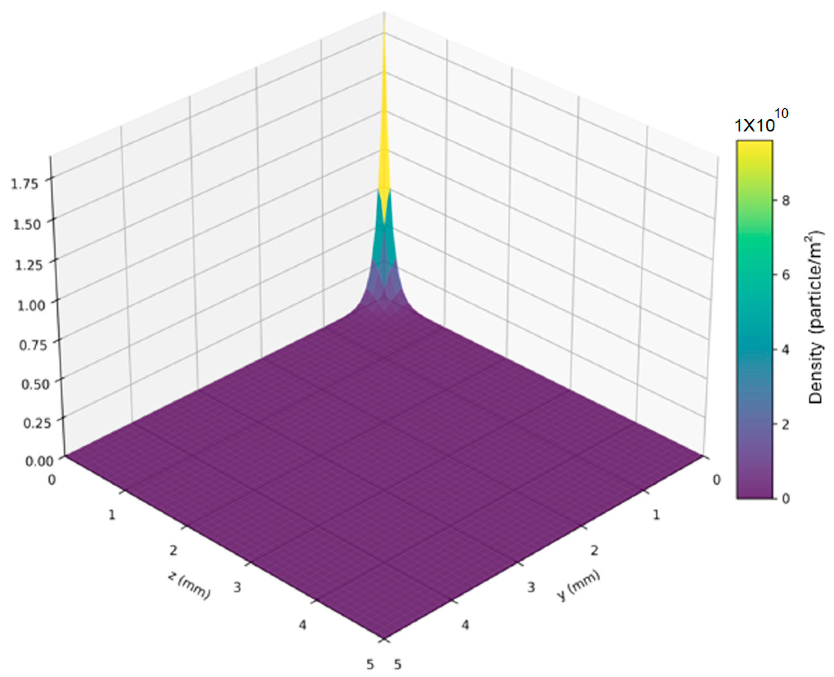
It is theoretically expected that, in the absence of mask interference, the deposited single-track profile or the number density of particles on the substrate should peak at the center (y = 0, z = 0) and decrease continuously outward [36]. If a sudden decline or an abrupt transition to zero in the track profile or the number density function is observed within the deposition region, the presence of an under-estimation issue can be inferred. To address this, the model utilizes a heatmap constructed from the number density of particles to precisely locate regions of abrupt decline, thereby delineating the under-estimated areas.
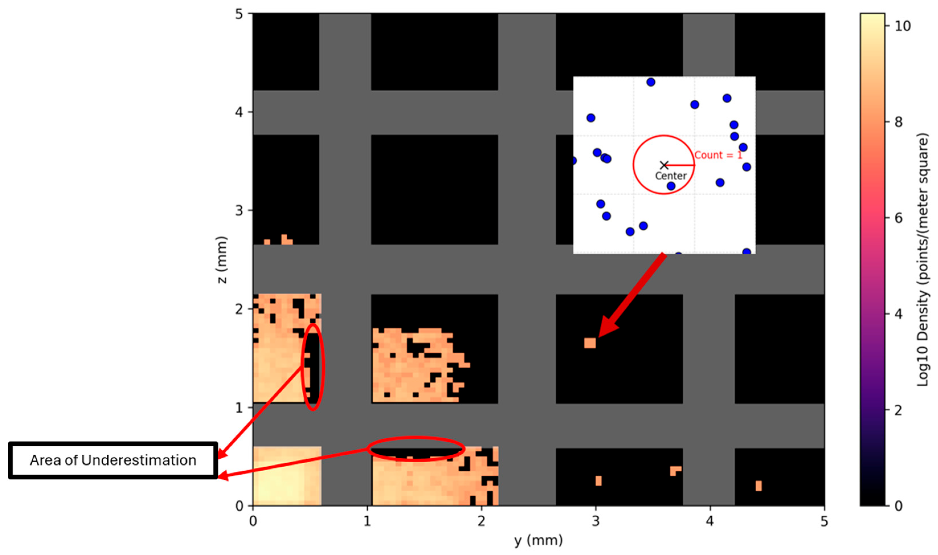
To generate the heatmap, first, the entire 5 mm × 5 mm region (a quarter of the substrate shown in Figure 1) is divided into a 2000 × 2000 grid. Next, each grid point is evaluated: if the point lies within the dead zone (as determined by physical priors), its number density is directly set to zero; otherwise, the local number density is computed by counting the number of predicted points (N) within a neighborhood of radius R c (Equation (A1)). To expedite the construction of the density map, a KD (k-dimensional) tree is employed for efficient neighborhood querying. Furthermore, to better accommodate the wide range of number density values, a smoothing transformation is applied to the data (Equation (A2)). The constant 1 in Equation (A2) is added to the number density values to prevent the logarithm from yielding negative infinity in regions where the number density is zero. Figure A1 presents the logarithmic density heatmap for a specific test sample (an inlet pressure of 4 MPa, an inlet temperature of 800 °C, a substrate SOD of 20 mm, a mask SOD of 16 mm, a mask wire diameter of 0.46 mm, a mask opening size of 1.14 mm, and an open area of 51%).
ρ c ( y , z ) = N π R c 2
ρ c , l o g = l o g 10 ρ c + 1
Figure A1. Logarithmic particle number density heatmap for the test sample (inlet pressure: 4 MPa, inlet temperature: 800 °C, substrate SOD: 20 mm, mask SOD: 16 mm, wire diameter: 0.46 mm, opening size: 1.14 mm, and open area: 51%).
Applsci 15 06418 g0a1
Subsequently, in regions outside the dead zone, effective areas are identified to correct the under-estimation issue, where regions expected to exhibit high number density are mistakenly predicted as low number density (see Figure A1). It is noteworthy that in Figure A1, the data have been subjected to a logarithmic transformation to promote overall smoothness; thus, any pronounced discontinuities observed in the log-density map can be reliably attributed to under-estimation.
To address this issue, first, the logarithmically transformed number density data are processed using the Otsu algorithm to automatically determine an optimal threshold [37]. The Otsu algorithm works by iteratively evaluating candidate thresholds: for each candidate, the data are divided into two groups (below and above the threshold), and the weight of each group is calculated as the proportion of data points in that group. The mean value for each group is computed, and then the between-class variance is calculated using
σ b 2 = w 0 w 1 μ 0 μ 1 2
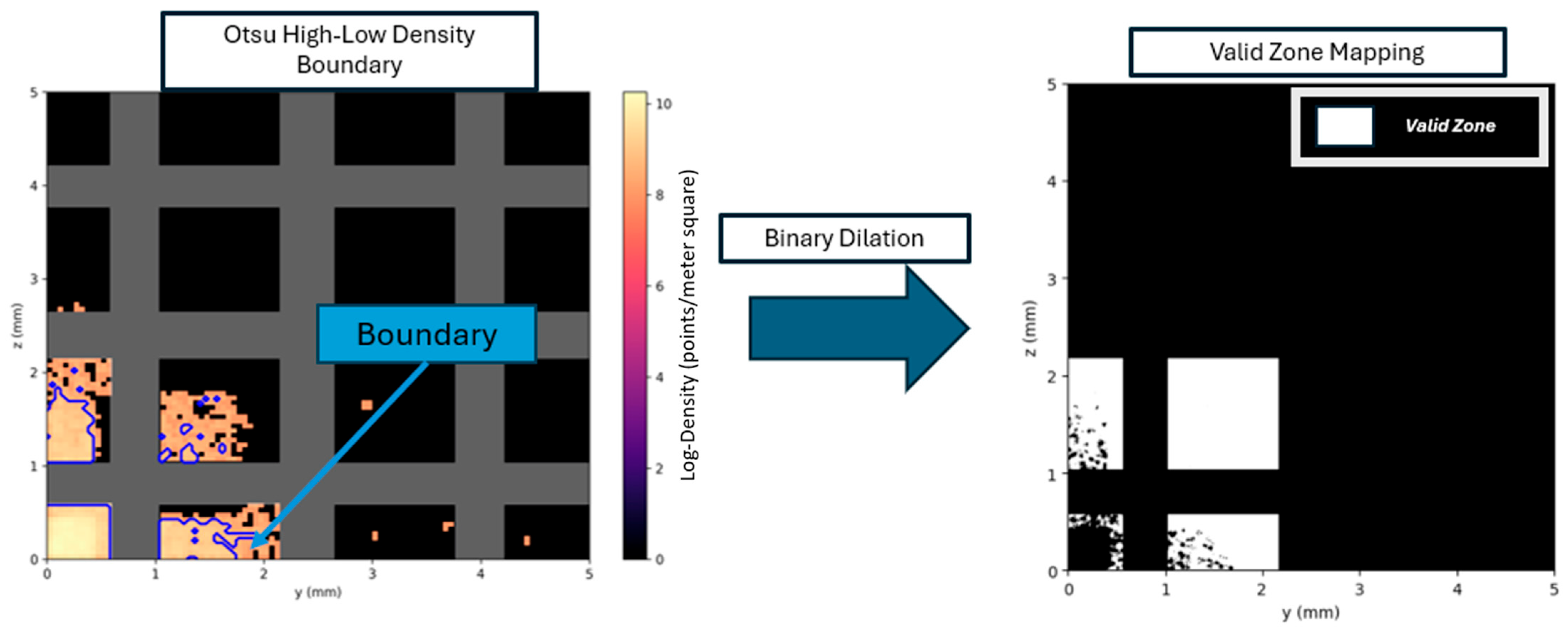
where w 0 and w 1 are the weights (proportions), and μ 0 and μ 1 are the means of the two groups, corresponding to low-number-density area and high-number-density area, respectively. The candidate threshold that maximizes the between-class variance is selected as the optimal threshold; moreover, a randomized search has been applied to further refine this selection. Regions with number density values exceeding this Otsu threshold are designated as high-number-density areas, while those with values falling below the threshold are labeled as low-number-density areas. In this context, only regions that are inherently characterized by low number density—namely, areas where an abrupt local drop in number density occurs adjacent to high-density regions, reflecting a dramatic local change—are considered to be under-estimated regions. Then, binary dilation is applied to the high-density areas until they extend to the dead zone boundaries. After this dilation, the low-density regions that fall within the expanded high-density areas are isolated by taking their intersection, which constitutes the valid region. This valid region, defined as the intersection of the expanded high-density area and the original low-density zone, represents the potential area for reallocating invalid prediction points that have erroneously fallen within the dead zone. Figure A2 illustrates this procedure: the left image highlights the initial identification of high-density regions, while the right image shows the result after expanding the high-density regions to the dead zone boundary and intersecting them with the low-density areas.
Figure A2. Morphological reconstruction of under-estimated regions for reallocation of invalid predictions.
Applsci 15 06418 g0a2
A key point to emphasize is that although the procedure described above effectively identifies regions of under-estimation, it does not inherently quantify the degree of under-estimation within each region. Thus, the subsequent phase provides a framework for assessing the relative severity of under-estimation across these regions, thereby determining which areas contain a greater or lesser number of invalid predictions that require reallocation.
As previously mentioned, in the absence of a mask, the deposited single-track profile or the probability density function of particle distribution on the substrate should exhibit a smooth, continuous decay [36]. The highest particle number density should be at the center, gradually decreasing with increasing radial distance. In other words, all the regions outside the dead zone are expected to follow this trend. This decay phenomenon is typically modeled by an exponential function, as such functions possess smooth, continuous, and monotonically decreasing properties that align well with the anticipated physical distribution. Based on this assumption, the data from the current valid prediction points are used to fit a target density function that characterizes the decay of particle number density as a function of the radial distance R ; that is, the density function is assumed to follow an exponential form. By applying a logarithmic transformation, this exponential relationship can be converted into a linear one, thereby facilitating parameter estimation and fitting. Subsequently, the fitted function is used to assign weights to each region within the valid zone identified in the earlier stage.
To be more specific, initially, radial statistics are computed for the predicted points within the deposition (effective) region. Specifically, the radial distance for each valid predicted point is calculated, as defined in
R i = y i 2 + z i 2
where R is the radial distance from the substrate center (y = 0 and z = 0), and y and z are the coordinates of the current point (location of each particle).
To quantify the number of particles in distinct radial intervals, the radial distance—from 0 to the maximum value—is partitioned into n intervals/bins:
b i n s = { 0 , R 1 , R 2 , , R m a x }
For each interval, the number of particles N is first computed, and the corresponding number density is then determined based on the annular area (Equation (A6)), yielding the number density ( ρ ) as defined in (Equation (A7)).
A r e a i = π ( R i + 1 2 R i 2 )
ρ i = N A r e a i
Subsequently, the logarithm of these number density values is calculated, and a linear regression is performed to establish the exponential relationship between radius and number density (Equation (A8)). Finally, the number density function ( ρ t a r g e t ) is constructed (Equation (A9)).
l n ρ = l n A B R
ρ t a r g e t ( R ) = A f i t e B R
Figure A3 illustrates the results for a specific test sample (with an inlet pressure of 4 MPa, an inlet temperature of 800 °C, a substrate SOD of 20 mm, a mask SOD of 16 mm, a mask wire diameter of 0.46 mm, a mask opening size of 1.14 mm, and an open area of 51%).
Figure A3. Radial number density heatmap and fitted exponential density function for the test sample (inlet pressure: 4 MPa, inlet temperature: 800 °C, substrate SOD: 20 mm, mask SOD: 16 mm, wire diameter: 0.46 mm, opening size: 1.14 mm, and open area: 51%).
Applsci 15 06418 g0a3
Although the target number density function—derived via the linear regression of the logarithmically transformed density against the radial distance—captures the general trend of decay from the center outward, noise and local prediction errors in the actual data may cause the fitted function to inadequately represent the maximum density expected in the central region. Consequently, to ensure that the candidate point selection strictly conforms to the physical prior (i.e., the central region should inherently exhibit a higher particle number density), an additional central bias factor, C , is introduced (Equation (A10)). This factor adjusts the weights of candidate points based on their radial distances, thereby amplifying the influence of those nearer to the center. In turn, during the local reallocation process, this central bias compensates for any discrepancies in the fitted function, ultimately yielding final predictions that more accurately reflect the true particle distribution.
C ( R i ) = ( R m a x R i R m a x ) γ
where R i is the radial distance of a candidate point, R m a x is the maximum radial distance, and γ (=2) is the exponent for the central bias factor.
Ultimately, the initial weight assigned to each candidate point in the under-estimated region is defined as the product of the target density function—obtained through fitting—and the central bias factor (Equation (A11)).
w i r a w = ρ t a r g e t ( R i ) × C ( R i )
Subsequently, the initial weight of each candidate point is normalized to yield the final weight
w i = w i r a w j = 1 N w j r a w
where N is the total number of invalid points. After computing and normalizing candidate point weights, a local reallocation strategy is applied to relocate invalid points from the dead zone into regions with under-estimated number density. For each invalid prediction within the dead zone, a KD-tree identifies a set of candidate locations in its local neighborhood, each assigned weights derived from the target density function and central bias. A probabilistic sampling approach then selects a candidate based on its normalized weight w i , conferring higher selection probability to points with larger weights. The chosen candidate’s coordinates replace the invalid prediction, thereby relocating the point from the dead zone to a physically plausible region.
This approach relocates each invalid point to a position more consistent with physical constraints. These corrected predictions are then combined with the valid ones to produce the final output set. By using a localized, weight-based probabilistic sampling strategy, the method effectively adjusts invalid points within the dead zone, preserving physical continuity and aligning the final predictions with the particle distribution seen in the training data.

Appendix B

Interpolation-Based Data-Augmentation Protocol for Expanding Sparse Process Parameters
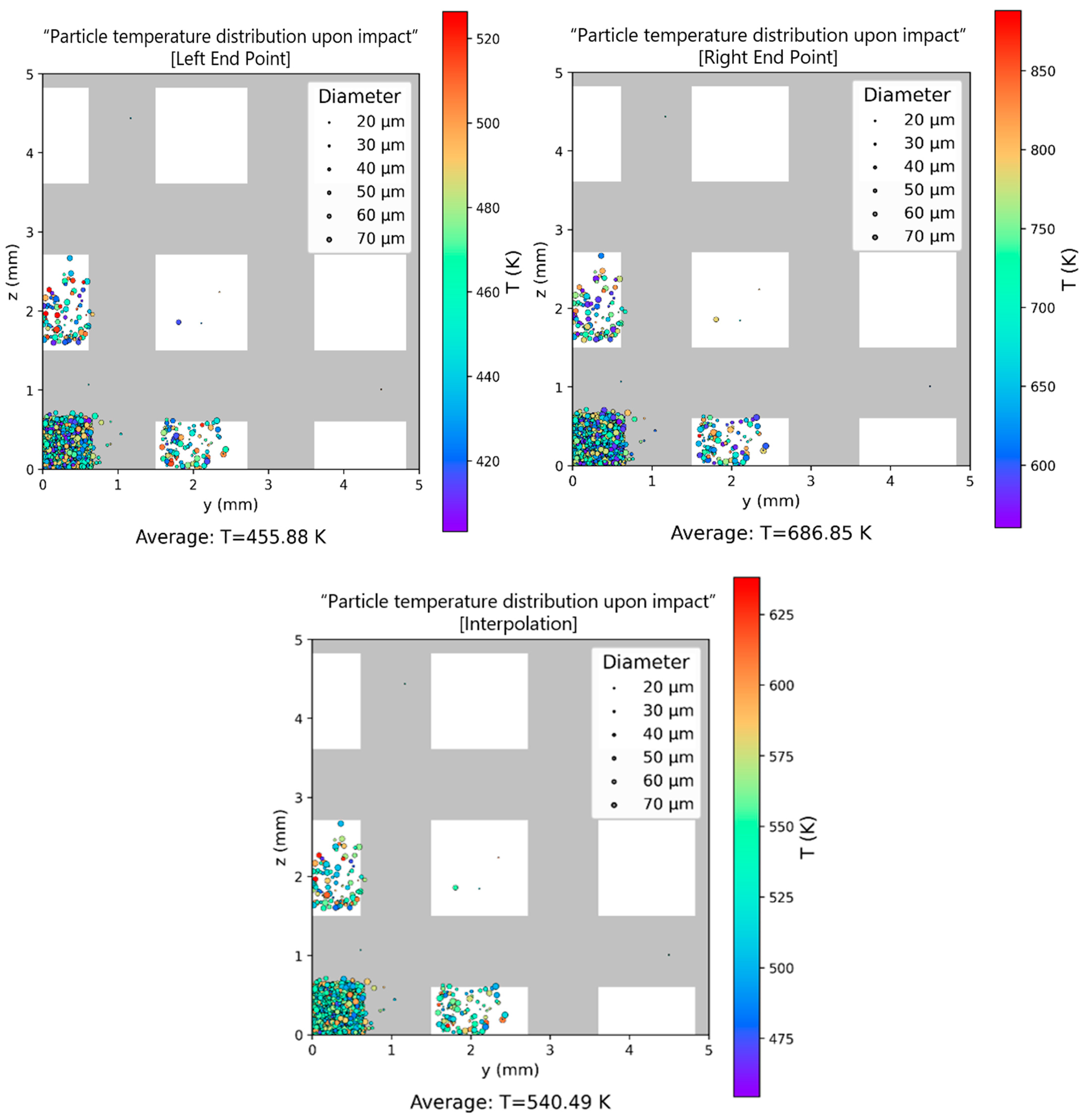
To perform interpolation, it is first necessary to select endpoint data from two or more sets of CFD simulations. However, particles in different simulations typically occupy different spatial positions or almost it is not possible to find two particles that share the same coordinates in two simulations. As a result, direct interpolation and matching are not feasible. To address this issue, stratified clustering is applied to each dataset based on the particles’ y-coordinates and sorted by z-coordinates within each y-based layer. This approach divides particles into multiple layers (strata) along the y- and z-axis.
Assume a CFD dataset contains N particles, where the coordinates of the i-th particle at the substrate are θ i = ( y i , z i ) , with y i and z i representing the y- and z-coordinates, respectively. To match particles within each layer, a relative difference distance based on the y-coordinate is defined to measure the similarity of particles in the horizontal direction (Equation (A13)). This ensures consistent stratification and enables effective interpolation within each corresponding layer.
Δ i , j = y i y j max y i , y j
where y i and y j are the y-coordinates of particles i and j . During the particle matching process, if the relative difference distance between two particles is less than or equal to 5%, they are considered to belong to the same group (Equation (A14)).
Δ i , j 0.05 G r o u p i = G r o u p j
After completing the matching process, the particle set for each layer is represented as S l (Equation (A15)). This set S l contains all the particles within a specific layer that have been grouped based on the matching criteria, ensuring that particles in the same layer share similar horizontal characteristics.
S l = { θ i y i y l m i n ,   y l m a x } ,   l = 1 ,   2 , , k
where [ y l m i n , y l m a x ) represents the range of y in the layer l , and k is the total number of layers. Furthermore, within each layer, particles are sorted by their z-coordinate to further divide the layer into y- and z-coordinate-based sublayers. Finally, particles from each dataset are matched based on these finalized sublayers, ensuring that each particle is spatially as close as possible to its counterpart in the other datasets.
The choice of interpolation method depends on the number of available data points and the dimensions that need to be considered. For different key parameters, different interpolation methods are applied. Since the total of 48 datasets includes only two distinct initial conditions (ICs), which involve two independent variables (gas temperature and pressure), linear interpolation (Equation (A16)) is the only feasible method. In this case, gas temperature and pressure are assumed to vary simultaneously with the same magnitude, collectively influencing the results. Additionally, among the 48 CFD datasets, there are only two sets of substrate standoff distances, so linear interpolation is also applied to this parameter. For the mask standoff distance, the interpolation method varies based on the available data. In the case of a 10 mm substrate, only two corresponding datasets (4 mm and 8 mm) exist [13], making linear interpolation appropriate. However, for the 20 mm substrate, there are four corresponding datasets for the masked SOD (4 mm, 8 mm, 12 mm, and 16 mm) [13]. In this scenario, spline interpolation (Equation (A17)), which offers greater precision than linear interpolation, is used.
Linear Interpolation
Y i X i = Y s t a r t + X i X e n d X e n d X s t a r t × Y e n d Y s t a r t
where X i is the input feature value at the interpolation point i and Y i is the interpolated output feature value at that point, X s t a r t and X e n d are the boundary input features, and Y s t a r t and Y e n d are the corresponding boundary output features.
4 Points Cubic Spline Interpolation
Y i X i = a 1 X i X 1 3 + b 1 X i X 1 2 + c 1 X i X 1 + d 1 , X X 1 , X 2 Y i X i = a 2 ( X i X 2 ) 3 + b 2 ( X i X 2 ) 2 + c 2 ( X i X 2 ) + d 2 , X X 2 , X 3 Y i ( X i ) = a 3 ( X i X 3 ) 3 + b 3 ( X i X 3 ) 2 + c 3 ( X i X 3 ) + d 3 , X [ X 3 , X 4 ]
where a n , b n , c n , and d n are cubic spline coefficients, and X 1 , X 2 , X 3 , and X 4 are the boundary points of the intervals.
Finally, for the mask type, each mask design includes multiple attributes, and the differences between masks are non-monotonic. Therefore, a weighted interpolation method (Equation (A18)) is applied, which considers multiple mask attributes and their irregular variations simultaneously, ensuring a more accurate representation of the data.
Inverse Distance Weighted (IDW)
Y i X i = k = 1 N w   Y   k = 1 N w k w k = 1 X i X k
where X i is the input feature value at the interpolation point i , X k is the coordinate vector (input feature values) of the k-th known point, Y k is the dependent/output variable value at the k-th known point, and Y i is the interpolated output feature value at the interpolation point.
It is worth mentioning that interpolation methods still have certain limitations and drawbacks. First, nearly all the interpolation techniques are highly sensitive to noise in the input data. Even small errors in the known data points can be amplified in the interpolation results [38]. Additionally, linear interpolation and cubic spline interpolation typically assume smooth transitions between data points, which may fail to capture abrupt changes or nonlinear behavior present in the actual data [39]. For IDW, unevenly distributed data can introduce bias, as distant points may have disproportionately high weights [40].
To mitigate these issues, an active learning strategy is implemented to filter and select interpolated data points with minimal noise for further processing. Before executing active learning, all the data is divided into a sample pool, validation set, and test set. The validation and test sets consist of the original 48 simulations (40 CFD simulation data for model validation and 8 CFD simulation data for final testing), while the sample pool is composed entirely of the interpolated data.
To ensure the interpolated data remains sufficiently distinct from the validation and test sets, two constraints are applied during the data generation. Firstly, the X (input feature) value for interpolation is determined based on a uniform step size, which is set such that each interpolated xm (the m-th element in the input feature) is at a 2% difference from the original boundary input feature values. This step size is used to sample all the X-values. Secondly, during the interpolation process, Gaussian noise is added to the corresponding y-values with a probability of 5% (Equation (A19)). These measures introduce meaningful variability into the interpolated data, thereby reducing the risk of overfitting and data leakage.
δ N 0 , σ 2 σ = Y e n d Y s t a r t × 5 % Y i = Y i + δ
where δ is a normally distributed random variable, σ is the standard deviation, σ 2 is the variance, Y i is the interpolated data before adding noise, and Y i is the interpolated data after adding noise. Based on these constraints, a total of 3040 interpolated datasets were generated. The predicted temperature distribution of particles on the substrate, considering a mask with a wire diameter of 0.89 mm, an opening size of 1.22 mm, and an open area of 33%, along with a substrate SOD of 10 mm and a mask SOD of 4 mm, under inlet conditions of 2.73 MPa and 619 °C, as well as the endpoints used for the interpolations, are presented in Figure A4.
Figure A4. Particle temperature distribution upon impact on the substrate, showing the left and right endpoints used for interpolation, along with the interpolation results.
Applsci 15 06418 g0a4
The process of refining and extracting interpolated data points with minimal noise through an active learning strategy involves several stages. The detailed workflow is illustrated in Figure A5. First, during the initialization phase, a validation set and an unlabeled data pool (candidate sample pool) are prepared. Then, a random subset of samples is selected from the sample pool to construct the initial labeled dataset for model training. To ensure randomness, the candidate sample pool is shuffled before selection. Next, the model is trained using the initialized labeled dataset, and the initial baseline error, measured as the Mean Squared Error (MSE), is calculated using the validation set. After the initialization phase, the process enters an iterative active learning stage. In each iteration, a small batch of candidate samples is temporarily added to the labeled dataset, and the model is retrained using this expanded set. The model’s performance is then re-evaluated on the validation set by computing the updated MSE. If the inclusion of the new batch results in a lower validation error compared to the previous baseline, the batch is permanently incorporated into the labeled dataset; otherwise, it is discarded. This cycle continues until all candidate samples have been assessed or a predefined performance threshold is achieved. Ultimately, the model with the lowest validation MSE is selected as the final model, and the corresponding refined labeled dataset is output for further use.
Figure A5. The detailed workflow for refining and extracting interpolated data points with minimal noise following an active learning strategy.
Applsci 15 06418 g0a5
In active learning, selecting the evaluation standard is crucial. An analysis of several models—decision tree, linear regression, and MLPRegressor—revealed differences in feature importance and model reliability. Notably, the decision tree model proved most robust; its performance deteriorated when nearly any feature was removed, indicating effective utilization of the entire feature set. In contrast, linear regression exhibited minimal change with most feature removals, suggesting reliance on only a few key features, while the MLPRegressor experienced negative R2 drops when certain features were omitted, implying suboptimal use of the full feature set. Consequently, the decision tree model is employed for active learning and further analysis due to its consistent and comprehensive performance.
The entire process is implemented using the decision tree model with default parameters from the scikit-learn library. A total of 86 datasets were ultimately selected, and the MSE of the decision tree model for the validation set and the test set were 53.6106 and 54.5309, respectively.

References

  1. Grujicic, M.; Zhao, C.L.; DeRosset, W.S.; Helfritch, D. Adiabatic Shear Instability Based Mechanism for Particles/Substrate Bonding in the Cold-Gas Dynamic-Spray Process. Mater. Des. 2004, 25, 681–688. [Google Scholar] [CrossRef]
  2. Yin, S.; Cavaliere, P.; Aldwell, B.; Jenkins, R.; Liao, H.; Li, W.; Lupoi, R. Cold Spray Additive Manufacturing and Repair: Fundamentals and Applications. Addit. Manuf. 2018, 21, 628–650. [Google Scholar] [CrossRef]
  3. Ashokkumar, M.; Thirumalaikumarasamy, D.; Sonar, T.; Deepak, S.; Vignesh, P.; Anbarasu, M. An Overview of Cold Spray Coating in Additive Manufacturing, Component Repairing and Other Engineering Applications. J. Mech. Behav. Mater. 2022, 31, 514–534. [Google Scholar] [CrossRef]
  4. Vo, P.; Martin, M. Layer-by-Layer Buildup Strategy for Cold Spray Additive Manufacturing. In Proceedings of the Proceedings of the International Thermal Spray Conference, Dusseldorf, Germany, 7–9 June 2017. [Google Scholar]
  5. Raoelison, R.N.; Verdy, C.; Liao, H. Cold Gas Dynamic Spray Additive Manufacturing Today: Deposit Possibilities, Technological Solutions and Viable Applications. Mater. Des. 2017, 133, 266–287. [Google Scholar] [CrossRef]
  6. Rahmati, S.; Jodoin, B. Physically Based Finite Element Modeling Method to Predict Metallic Bonding in Cold Spray. J. Therm. Spray Technol. 2020, 29, 611–629. [Google Scholar] [CrossRef]
  7. Smith, M.F. Introduction to Cold Spray. In High Pressure Cold Spray; Springer International Publishing: Cham, Switzerland, 2016; pp. 1–16. [Google Scholar]
  8. Papyrin, A.; Kosarev, V.; Klinkov, S.; Alkimov, A.; Fomin, V. Cold Spray Technology; Elsevier: Amsterdam, The Netherlands, 2007; ISBN 9780080451558. [Google Scholar]
  9. Wang, S.; Lu, A.; Zhong, C.-J. Hydrogen Production from Water Electrolysis: Role of Catalysts. Nano Converg. 2021, 8, 4. [Google Scholar] [CrossRef]
  10. Aghasibeig, M.; Dolatabadi, A.; Wuthrich, R.; Moreau, C. Three-Dimensional Electrode Coatings for Hydrogen Production Manufactured by Combined Atmospheric and Suspension Plasma Spray. Surf. Coat. Technol. 2016, 291, 348–355. [Google Scholar] [CrossRef]
  11. Aghasibeig, M.; Monajatizadeh, H.; Bocher, P.; Dolatabadi, A.; Wuthrich, R.; Moreau, C. Cold Spray as a Novel Method for Development of Nickel Electrode Coatings for Hydrogen Production. Int. J. Hydrogen Energy 2016, 41, 227–238. [Google Scholar] [CrossRef]
  12. Aghasibeig, M.; Moreau, C.; Dolatabadi, A.; Wuthrich, R. Engineered Three-Dimensional Electrodes by HVOF Process for Hydrogen Production. J. Therm. Spray Technol. 2016, 25, 1561–1569. [Google Scholar] [CrossRef]
  13. Nasire, N.; Jadidi, M.; Dolatabadi, A. Numerical Analysis of Cold Spray Process for Creation of Pin Fin Geometries. Appl. Sci. 2024, 14, 11147. [Google Scholar] [CrossRef]
  14. Bobzin, K.; Wietheger, W.; Heinemann, H.; Dokhanchi, S.R.; Rom, M.; Visconti, G. Prediction of Particle Properties in Plasma Spraying Based on Machine Learning. J. Therm. Spray Technol. 2021, 30, 1751–1764. [Google Scholar] [CrossRef]
  15. Canales, H.; Cano, I.G.; Dosta, S. Window of Deposition Description and Prediction of Deposition Efficiency via Machine Learning Techniques in Cold Spraying. Surf. Coat. Technol. 2020, 401, 126143. [Google Scholar] [CrossRef]
  16. Eberle, M.; Pinches, S.; Guzman, P.; King, H.; Zhou, H.; Ang, A. Application of Machine Learning for the Prediction of Particle Velocity Distribution and Deposition Efficiency for Cold Spraying Titanium Powder. Comput. Mater. Sci. 2024, 244, 113224. [Google Scholar] [CrossRef]
  17. Malamousi, K.; Delibasis, K.; Allcock, B.; Kamnis, S. Digital Transformation of Thermal and Cold Spray Processes with Emphasis on Machine Learning. Surf. Coat. Technol. 2022, 433, 128138. [Google Scholar] [CrossRef]
  18. Samareh, B.; Dolatabadi, A. A Three-Dimensional Analysis of the Cold Spray Process: The Effects of Substrate Location and Shape. J. Therm. Spray Technol. 2007, 16, 634–642. [Google Scholar] [CrossRef]
  19. Sheather, S.J.; Jones, M.C. A Reliable Data-Based Bandwidth Selection Method for Kernel Density Estimation. J. R. Stat. Soc. Ser. B Stat. Methodol. 1991, 53, 683–690. [Google Scholar] [CrossRef]
  20. Kullback, S.; Leibler, R.A. On Information and Sufficiency. Ann. Math. Stat. 1951, 22, 79–86. [Google Scholar] [CrossRef]
  21. Blei, D.M.; Kucukelbir, A.; McAuliffe, J.D. Variational Inference: A Review for Statisticians. J. Am. Stat. Assoc. 2017, 112, 859–877. [Google Scholar] [CrossRef]
  22. Alonso, L.; Garrido-Maneiro, M.A.; Poza, P. A Study of the Parameters Affecting the Particle Velocity in Cold-Spray: Theoretical Results and Comparison with Experimental Data. Addit. Manuf. 2023, 67, 103479. [Google Scholar] [CrossRef]
  23. Brunton, S.L.; Noack, B.R.; Koumoutsakos, P. Machine Learning for Fluid Mechanics. Annu. Rev. Fluid Mech. 2020, 52, 477–508. [Google Scholar] [CrossRef]
  24. Bengio, Y.; Courville, A.; Vincent, P. Representation Learning: A Review and New Perspectives. IEEE Trans. Pattern Anal. Mach. Intell. 2013, 35, 1798–1828. [Google Scholar] [CrossRef]
  25. Breiman, L.; Friedman, J.H.; Olshen, R.A.; Stone, C.J. Classification and Regression Trees; Routledge: New York, NY, USA, 2017; ISBN 9781315139470. [Google Scholar]
  26. Box, G.E.P.; Cox, D.R. An Analysis of Transformations. J. R. Stat. Soc. Ser. B Stat. Methodol. 1964, 26, 211–243. [Google Scholar] [CrossRef]
  27. Hinton, G.E.; Salakhutdinov, R.R. Reducing the Dimensionality of Data with Neural Networks. Science 2006, 313, 504–507. [Google Scholar] [CrossRef]
  28. Schmidt, T.; Gärtner, F.; Assadi, H.; Kreye, H. Development of a Generalized Parameter Window for Cold Spray Deposition. Acta Mater. 2006, 54, 729–742. [Google Scholar] [CrossRef]
  29. Garmeh, S.; Jadidi, M.; Lamarre, J.-M.; Dolatabadi, A. Cold Spray Gas Flow Dynamics for On and Off-Axis Nozzle/Substrate Hole Geometries. J. Therm. Spray Technol. 2023, 32, 208–225. [Google Scholar] [CrossRef]
  30. Rahmati, S.; Zúñiga, A.; Jodoin, B.; Veiga, R.G.A. Deformation of Copper Particles upon Impact: A Molecular Dynamics Study of Cold Spray. Comput. Mater. Sci. 2020, 171, 109219. [Google Scholar] [CrossRef]
  31. Zhang, L.; Chen, X.; Zhou, W.; Cheng, T.; Chen, L.; Guo, Z.; Han, B.; Lu, L. Digital Twins for Additive Manufacturing: A State-of-the-art Review. Appl. Sci. 2020, 10, 8350. [Google Scholar] [CrossRef]
  32. Bergs, T.; Gierlings, S.; Auerbach, T.; Klink, A.; Schraknepper, D.; Augspurger, T. The Concept of Digital Twin and Digital Shadow in Manufacturing. Procedia CIRP 2021, 101, 81–84. [Google Scholar] [CrossRef]
  33. Mukherjee, T.; DebRoy, T. A Digital Twin for Rapid Qualification of 3D Printed Metallic Components. Appl. Mater. Today 2019, 14, 59–65. [Google Scholar] [CrossRef]
  34. Tao, F.; Qi, Q.; Wang, L.; Nee, A.Y.C. Digital Twins and Cyber–Physical Systems toward Smart Manufacturing and Industry 4.0: Correlation and Comparison. Engineering 2019, 5, 653–661. [Google Scholar] [CrossRef]
  35. Petrovskiy, A.; Arifeen, M.; Petrovski, S. The Use of Machine Learning for Digital Shadowing in Thermal Spray Coating. In Proceedings of the Seventh International Scientific Conference “Intelligent Information Technologies for Industry” (IITI’23); Lecture Notes in Networks and Systems. Springer Science and Business Media Deutschland GmbH: Cham, Switzerland, 2023; Volume 776, pp. 343–352, ISBN 9783031437885. [Google Scholar]
  36. Ikeuchi, D.; Vargas-Uscategui, A.; Wu, X.; King, P.C. Neural Network Modelling of Track Profile in Cold Spray Additive Manufacturing. Materials 2019, 12, 2827. [Google Scholar] [CrossRef] [PubMed]
  37. Otsu, N. A Threshold Selection Method from Gray-Level Histograms. IEEE Trans. Syst. Man Cybern. 1979, 9, 62–66. [Google Scholar] [CrossRef]
  38. Ramani, S.; Thevenaz, P.; Unser, M. Regularized Interpolation For Noisy Data. In Proceedings of the 2007 4th IEEE International Symposium on Biomedical Imaging: From Nano to Macro, Arlington, VA, USA, 12–15 April 2007; pp. 612–615. [Google Scholar]
  39. Lehmann, T.M.; Gonner, C.; Spitzer, K. Survey: Interpolation Methods in Medical Image Processing. IEEE Trans. Med. Imaging 1999, 18, 1049–1075. [Google Scholar] [CrossRef] [PubMed]
  40. Achilleos, G. Errors within the Inverse Distance Weighted (IDW) Interpolation Procedure. Geocarto Int. 2008, 23, 429–449. [Google Scholar] [CrossRef]
Figure 1. Overview of the CFD simulations performed for a masked cold spray process under various operating conditions [13]. It illustrates the nozzle geometry, four different masks, and a sample CFD result depicting particle normal velocity upon impact on the substrate. These CFD data serve as the training dataset for the ML models.
Applsci 15 06418 g001
Figure 2. Workflow of the ML model training and development process.
Applsci 15 06418 g002
Figure 3. Schematic illustration of the stratified and greedy sampling process. The differently colored particles simply represent distinct individuals within the population.
Applsci 15 06418 g003
Figure 4. Flow diagram of genetic algorithm.
Applsci 15 06418 g004
Figure 5. Overly dispersed sampling distribution (excessive bandwidth).
Applsci 15 06418 g005
Figure 6. Overly concentrated sampling distribution (insufficient bandwidth).
Applsci 15 06418 g006
Figure 7. Overall optimization workflow for the first submodule.
Applsci 15 06418 g007
Figure 8. (a) KNN-KDE-based prediction vs. ground truth distribution along the y- and z-axes for the test sample (inlet pressure: 4 MPa, inlet temperature: 800 °C, substrate SOD: 20 mm, mask SOD: 16 mm, wire diameter: 0.46 mm, opening size: 1.14 mm, and open area: 51%). Where the bars overlap, they appear as a purple. This indicates where the predicted distribution closely matches the ground truth; (b) predicted particle spatial distribution by KNN+KDE for the same test sample.
Applsci 15 06418 g008
Figure 9. Feature importance analysis using the “dropping feature” method, where the decrease in R2 indicates the impact of removing each feature.
Applsci 15 06418 g009
Figure 10. Feature importance analysis using the “dropping feature” method after adding the interpolated data, where the decrease in R2 indicates the impact of removing each feature.
Applsci 15 06418 g010
Figure 11. Dataset partitioning for model training.
Applsci 15 06418 g011
Figure 12. An example of a symbolic regression.
Applsci 15 06418 g012
Figure 13. The workflow of the symbolic regression process.
Applsci 15 06418 g013
Figure 14. Dataset partitioning for model optimization.
Applsci 15 06418 g014
Figure 15. Optimization and weighting process for the weighted random forest model.
Applsci 15 06418 g015
Figure 16. (a) Distribution of reallocated predictions vs. ground truth (y and z) for the test sample (inlet pressure: 4 MPa, inlet temperature: 800 °C, substrate SOD: 20 mm, mask SOD: 16 mm, wire diameter: 0.46 mm, opening size: 1.14 mm, and open area: 51%). Where the bars overlap, they appear as a purple. This indicates where the predicted distribution closely matches the ground truth; (b) local reallocation of under-estimated predictions for the mentioned test sample.
Applsci 15 06418 g016
Figure 17. Scatter plot of the second model: predicted vs. actual values on the entire test set.
Applsci 15 06418 g017
Figure 18. Ground truth for the specific test sample: an inlet pressure of 4 MPa, an inlet temperature of 800 °C, a substrate SOD of 20 mm, a mask SOD of 16 mm, a mask wire diameter of 0.46 mm, a mask opening size of 1.14 mm, and an open area of 51%.
Applsci 15 06418 g018
Figure 19. Predictions of the 2nd model for the specific test sample: an inlet pressure of 4 MPa, an inlet temperature of 800 °C, a substrate SOD of 20 mm, a mask SOD of 16 mm, a mask wire diameter of 0.46 mm, a mask opening size of 1.14 mm, and an open area of 51%.
Applsci 15 06418 g019
Figure 20. Predictions from the integrated first and second models for the specific test sample: inlet pressure of 4 MPa, inlet temperature of 800 °C, substrate SOD of 20 mm, mask SOD of 16 mm, mask wire diameter of 0.46 mm, mask opening size of 1.14 mm, and an open area of 51%.
Applsci 15 06418 g020
Table 1. Genetic algorithm hyperparameters.
HyperparameterValue
Max generations20
Population size30
Mutation rate0.1
Table 2. Global Var/mean ratio (genetic algorithm).
Feature NameGlobal Var RatioGlobal Mean Ratio
y1.019941.00214
z1.02871.01776
Diameter0.985841.00052
u0.982060.99928
v1.138940.99796
w1.1490021.1052
T0.988381.0006
Table 3. Optimal transformations for each feature.
FeatureMath Transformation
Diameterx
y-Coordinate c o s x
z-Coordinatesqrt(cos(x))
Wire Diameter x
Opening Size 2 x
Open Area Percent x / x x
Pressure x 2 x
Temperature x
Substrate Standoff Distance x 2
Mask Standoff Distance x
Table 4. The parameters used for multi-symbolic regressions.
HyperparametersValues
Initial Population500
End Population50
Max Generation5
Cross over Rate0.7
Mutate Rate0.3
Max Depth4
Table 5. Optimized hyperparameters of the random forest model.
HyperparametersValues
N estimators200
Max depthNone (Unlimited)
Min samples split2
Min samples leaf1
Max featuresNone (Unlimited)
Disclaimer/Publisher’s Note: The statements, opinions and data contained in all publications are solely those of the individual author(s) and contributor(s) and not of MDPI and/or the editor(s). MDPI and/or the editor(s) disclaim responsibility for any injury to people or property resulting from any ideas, methods, instructions or products referred to in the content.