Abstract
Optimizing vehicle placement in unmarked parking areas is essential for maximizing space efficiency, particularly in irregular and high-demand urban environments. This study investigates the optimal allocation of additional vehicles in spaces left unoccupied around parked cars by comparing seven heuristic optimization algorithms: Particle Swarm Optimization, Artificial Bee Colony, Gray Wolf Optimizer, Harris Hawks Optimizer, Phasor Particle Swarm Optimization, Multi-Population Based Differential Evolution, and the Colony-Based Search Algorithm. The experiments were conducted in two different parking areas, one designed for parallel parking and the other for perpendicular parking, under three scenarios allowing different levels of cars’ rotational flexibility. The results indicate that MDE consistently outperforms other methods in both speed and robustness, achieving the highest vehicle capacity. These findings provide a foundation for smart parking systems, enabling real-time optimization, reduced congestion, and improved urban mobility.
1. Introduction
The increasing number of vehicles in modern cities has made parking demand and search times a critical issue. This situation leads to negative consequences such as fuel waste, traffic congestion, and environmental pollution, adversely affecting both individual drivers and urban transportation systems. Within the scope of smart city applications, the efficient utilization of parking areas has become an essential requirement for traffic management. An effective parking management system not only reduces the time drivers spend searching for parking spaces but also improves traffic flow while minimizing fuel consumption and environmental impact. In this context, accurately identifying available parking spaces and optimally positioning vehicles is a fundamental necessity for developing effective solutions.
Traditional parking management systems are effective in detecting occupancy status in designated, line-marked parking areas. However, they are inadequate for unmarked parking spaces, such as roadside parking, event venues, and temporary parking arrangements, where the number of vehicles that can fit and their potential positions are uncertain. Existing systems primarily focus on identifying parking occupancy without providing guidance to ensure the most efficient use of available spaces. Zhou et al. [1] examined parking areas in Lviv’s historic city center and highlighted that simple IoT (Internet of Things) solutions were insufficient for unmarked parking spaces, necessitating more advanced systems. Similarly, Plasencia-Lozano and Méndez-Manjón [2] compared the efficiency of marked and unmarked parking areas, demonstrating that unmarked spaces suffer from significant capacity losses due to randomly positioned vehicles.
Mathematical modeling and simulation studies have indicated that, while fixed-length constraints in marked parking areas can lead to inefficiencies, random parking behavior in unmarked spaces can reduce capacity utilization [3]. Ismael et al. [4] found that parking accessibility for different vehicle types directly affects traffic flow and environmental costs, with limited parking availability increasing search times and exacerbating congestion. Xu and Skiena [5] and Xu [6] suggested that unmarked parking areas offer more flexible solutions than fixed-size parking lines. However, they emphasized that without an appropriate optimization strategy, this advantage cannot be fully utilized. These findings indicate the need for novel approaches, particularly in cities like Kayseri, where a significant portion of roadside parking areas are unmarked.
Although the optimization problem addressed in this study is inherently nonconvex due to vehicle rotation, buffer zones, spatial overlap constraints, and irregular parking boundaries, it is conceptually valuable to acknowledge the role of convex optimization techniques under idealized conditions. For instance, equality-constrained quadratic programming has been successfully applied in structured spatial estimation problems [7]. While originally developed for direction-of-arrival estimation, its mathematical formulation illustrates how convex approaches can yield global optima in environments with well-defined and continuous constraints.
In the presented context, one can imagine hypothetical scenarios where all vehicles are identical, parking areas are rectangular and symmetric, and no rotation is permitted. In such simplified cases, multiple vehicle configurations (e.g., symmetric placements in mirrored subspaces) could produce equivalent or optimal results. If the objective were limited to minimizing maneuver time or maximizing vehicle count with continuous variables and smooth constraints, a convex relaxation might, in theory, offer a tractable formulation. However, real-world parking scenarios involve multiple vehicle types, variable rotation angles, and discontinuous feasibility conditions. These features result in a multimodal and fragmented solution space, which makes heuristic and swarm-based methods far more suitable in practice.
Optimization methods have been employed for various purposes in parking management. Advanced algorithms have been developed for dynamic parking allocation [8], and the integration of electric vehicle parking areas with power grids has been optimized [9,10]. Parking lot layouts and capacity have been improved by optimizing underground parking structures and corridor designs [11], and routing strategies have been developed [12]. Research on shared mobility has examined the optimal placement of shared vehicles and their impact on urban traffic [13,14,15], while algorithms have been proposed to reduce the time drivers spend searching for parking [16]. Studies comparing the efficiency of marked and unmarked parking areas have evaluated the impact of different parking designs on vehicle capacity [2]. Additionally, research on parking angle optimization has aimed to determine the most suitable angles for specific parking layouts, showing that optimizing angles can significantly increase capacity [17].
In order to inform users about available parking spaces, it is first necessary to detect whether a parking spot is occupied or vacant. To achieve this, either sensor-based systems or image processing techniques are commonly employed [18,19]. Examples of sensor-based approaches include magnetic sensors and smart cameras as used by [20], WSN (Wireless Sensor Network)-based sensors [21], optical and magnetic sensors [22], and LIDAR (Light Detection and Ranging) technology [23]. In image-based studies, various deep learning models have been utilized such as Deep Convolutional Neural Networks (DCNNs) [24], Faster Region-based Convolutional Neural Networks (Faster R-CNNs) [25], Residual Networks (ResNet50) [26], Mask Region-based Convolutional Neural Networks (Mask R-CNNs) [27], and YOLO (You Only Look Once) models [28,29,30]. For the optimization problem addressed in this study, a vision-based segmentation approach is necessary, similar to the study by Janowski et al. [31], which integrates YOLO and optimization techniques. This allows for the detection of vehicle boundaries, making it possible to perform optimization based on the remaining available space. Although many mobile applications, such as ISPARK [32] and IstPark [33], that show users available parking spots are becoming increasingly common in various cities, there are only a few examples that provide real-time solutions for unmarked areas. For unmarked parking areas, the SONAH [34] parking management system and the concept proposed by Janowski, Hüsrevoğlu, and Renigier-Bilozor [31] are rare examples.
Most existing studies have either focused on detecting parking occupancy or optimizing marked parking spaces. A comprehensive heuristic optimization comparison to maximize vehicle capacity in unmarked parking areas remains lacking. Janowski, Hüsrevoğlu, and Renigier-Bilozor [31] developed the SPARK (Smart Parking Assistance and Resource Knowledge) system, which integrates YOLO v9 image segmentation with the ABC (Artificial Bee Colony) optimization algorithm to optimize vehicle placement in unmarked parking areas. However, this study did not compare different heuristic methods or consider varying vehicle sizes.
This study aims to compare seven heuristic optimization algorithms—Particle Swarm Optimization (PSO), Phasor Particle Swarm Optimization (PPSO), ABC, Gray Wolf Optimizer (GWO), Harris Hawks Optimization (HHO), Multi-Population Based Differential Evolution (MDE), and the Colony-Based Search Algorithm (CSA)—to maximize the utilization of available spaces in unmarked parking areas. The performance of these algorithms will be evaluated in terms of speed and efficiency, and their impact on parking optimization for different vehicle types will be analyzed.
To achieve this, three different parking scenarios are considered: (1) parallel parking optimization, (2) parking at angles between 0° and 45°, and (3) free-angle parking between 0° and 180°. The algorithms’ performances are assessed based on computational time, space utilization, and maximum vehicle capacity. The study is conducted using vehicles of different sizes, including the Citroën Ami (Stellantis, Paris, France) and Volkswagen Crafter (Volkswagen AG, Wolfsburg, Germany), and is tested through computer simulations based on real-world parking scenarios in Kayseri.
The results reveal significant performance differences among the heuristic optimization methods for unmarked parking areas. The findings highlight that selecting the most suitable algorithm for vehicle placement optimization in unmarked parking areas is critical for urban sustainability and traffic management.
While most existing systems address parking space detection and vehicle positioning, fewer studies emphasize the role of parking management as part of broader public space governance. This dimension becomes especially important in light of fiscal and spatial planning perspectives.
As Grover and Walacik [35] underline, “the local public services (funded by property taxes) are highly visible with the population having a direct experience of them and their management”, which reinforces the relevance of systems like data-driven vehicle placement optimizers that dynamically reflect the real-time use of public urban space. Moreover, as highlighted by Chmielewska et al. [36], urban governance is a critical factor for the success of urban development, requiring transparency, inclusivity, and coherent policy frameworks. In this context, the proposed heuristic optimization framework for unmarked parking areas not only provides technical functionality but also contributes to the broader urban governance landscape by offering actionable spatial data that can inform equitable and sustainable city planning.
In the following sections of this paper, the performance analyses of the optimization algorithms will be presented, and the obtained findings will be discussed.
2. Materials and Methods
This section describes the study areas, vehicle dimensions, and theoretical background of the optimization methods used to optimally allocate additional vehicles in the remaining spaces of unmarked parking areas. To compare optimization performance, the PSO, PPSO, ABC, GWO, HHO, MDE, and CSA methods were evaluated.
2.1. Study Area and Data Acquisition
The study was conducted in two real-world parking areas located in the Alparslan neighborhood of Kayseri, Türkiye. These selected parking areas do not have predefined parking lines. The geometric properties of the parking areas, as well as the positions and dimensions of the vehicles within them, were prepared in shapefile format for analysis. A sample dataset was developed based on an initial vehicle arrangement, in which the vehicles were randomly placed, aiming to maximize the number of additional vehicles placed in the remaining empty spaces. This approach realistically reflects the complex spatial arrangement challenges commonly encountered in unmarked parking areas due to irregular geometries and varying vehicle sizes.
The selected parking areas and the occupied vehicle zones are illustrated in Figure 1.
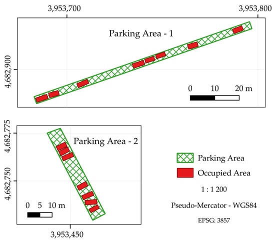
Figure 1.
Parking areas and occupied spaces (Source: author’s own elaboration).
The first parking area is a roadside section designated for parallel parking, measuring approximately 93.25 m in length and 3.00 m in width, with a total area of approximately 279.74 m2. The second parking area is a designated section within a parking lot intended for perpendicular parking. This area measures approximately 5.75 m in width and 39.70 m in length, with a total area of approximately 227.01 m2.
2.2. Vehicles and Size Constraints
To demonstrate the effectiveness of the proposed parking optimization, three different vehicle types were considered:
- Citroën Ami [37]—A small electric vehicle selected for its compact dimensions, which provide an advantage in narrow or irregular parking spaces.
- Volkswagen Crafter [38]—A large van chosen to illustrate the challenges associated with parking oversized vehicles.
- Standard Vehicle—A reference vehicle with typical width and length dimensions, used for comparison purposes.
In the optimization process, the most efficient parking arrangement was sought for each scenario, accommodating one Ami, one Crafter, and as many standard vehicles as possible.
In this study, the reference vehicle width was set at 2.05 m [39]. To ensure safe parking and prevent potential collisions, additional safety buffers were incorporated into each vehicle’s dimensions to account for real-world maneuvering clearances. A buffer of 0.30 m was added to each side of the vehicles (resulting in a total of 0.60 m when two vehicles are adjacent), and a 0.20 m buffer was added to the front (totaling 0.40 m when two vehicles are parked facing each other). In Türkiye, the minimum parking space width is generally specified as between 2.40 m and 2.50 m according to various regulations [40]. This range is considered suitable for studies where the objective is to accommodate as many vehicles as possible within a given area. These safety buffers were integrated into the optimization model, effectively expanding each vehicle’s occupied space and ensuring that the generated solutions are both feasible and safe for real-world implementation. The actual vehicle dimensions, along with the adjusted dimensions including the safety buffers, are presented in Table 1.

Table 1.
Vehicle dimensions.
2.3. Parking Scenarios
Three scenarios were defined to represent increasing levels of complexity in vehicle placement and rotation:
Scenario 1: Parallel Parking Without Rotation (Parking Area 1)
- Focuses on positioning vehicles in a strictly parallel manner, effectively treating each parking spot as having zero rotational freedom.
- Aims to assess how effectively the algorithms place vehicles when rotation is restricted to a single axis.
Scenario 2: Parallel Parking with Limited Rotation Up to 45° (Parking Area 1)
- Extends the first scenario by allowing limited rotation—up to 45° from the reference axis.
- Highlights how partial rotation flexibility can improve space utilization and influence algorithmic performance.
Scenario 3: Perpendicular Parking with Full Rotation (Parking Area 2)
- Introduces the highest level of complexity by permitting any rotation angle between 0° and 180°.
- Includes additional complexity due to the inability of a Volkswagen Crafter to fit perpendicularly into the parking space.
2.4. Outline of Computational Approach
The optimization process was designed to maximize the number of vehicles placed within the available parking space while ensuring an optimal arrangement. The optimization framework was derived from the study by Janowski, Hüsrevoğlu, and Renigier-Bilozor [31] and extended with new heuristic methods, additional vehicle types (the Citroën Ami and Volkswagen Crafter), and vertical parking configurations. These modifications allow for a more comprehensive evaluation of vehicle placement strategies, particularly in unmarked parking areas.
The optimization experiments were conducted using a laptop equipped with a 13th Gen Intel(R) Core(TM) i9-13900HX, 2.20 GHz processor, 64 GB DDR5 RAM, and the Windows 11 operating system, utilizing Python 3.12 as the primary programming language.
The fundamental principle of the optimization methods is to achieve the best solution by minimizing or maximizing a predefined objective (cost) function. In this study, the optimization process is based on the approach developed by Janowski, Hüsrevoğlu, and Renigier-Bilozor [31] for vehicle placement in unmarked parking areas. This approach consists of three key components:
Decision Variables: These define the position of potential parking spaces (, coordinates) and the rotation angle () of vehicles. The optimization process iteratively adjusts these variables to maximize vehicle capacity. The optimization algorithm determines the best configuration for parking spaces, forming a solution space of size [31].
Constraints: To ensure realistic parking arrangements, the following constraints from [31] are imposed:
- Vehicles must be positioned within the parking area boundaries.
- Newly placed vehicles must not overlap with existing occupied spaces.
- Overlapping between newly placed vehicles must be avoided.
These constraints are enforced through geometric analysis, in–out checks, and vector-based intersection calculations.
Cost Function (Objective Function): This function plays a critical role in evaluating the quality of the parking arrangement and penalizing improper placements. The cost function is adapted directly from Janowski, Hüsrevoğlu, and Renigier-Bilozor [31] and is defined as follows:
where [31]:
- M is the number of vehicles.
- Pout represents the penalty for vehicles positioned outside the parking area (penalty cost = 5000).
- Iout,i is an indicator function that equals 1 if the i-th vehicle is outside the parking area, and 0 otherwise.
- Poccupied is the penalty per percentage of overlap with an already occupied space (penalty cost = 300).
- OPoccupied,i is the percentage overlap of the i-th vehicle with an occupied area.
- Pnew is the penalty per percentage of overlap with another new vehicle (penalty cost = 300).
- OPnew,ij is the percentage overlap between the i-th and j-th vehicles [31].
In the optimization process, each solution is represented as a row vector. These row vectors are constructed based on the number of vehicles and the number of decision variables computed for each vehicle. Each solution vector is expressed as a row vector of length , where for Scenario 1 (with only the and coordinates computed) and for the other scenarios (with the and coordinates as well as the rotation angle computed); that is,
The solution set formed by vertically stacking these row vectors is expressed as
At each iteration, these solution vectors are updated according to the internal dynamics of the optimization method until the predefined stopping criteria are met. Throughout the process, the best solution encountered is retained as the global best solution.
The optimization workflow for searching for the optimal and maximum number of parked vehicles for each method and scenario is illustrated in Figure 2.
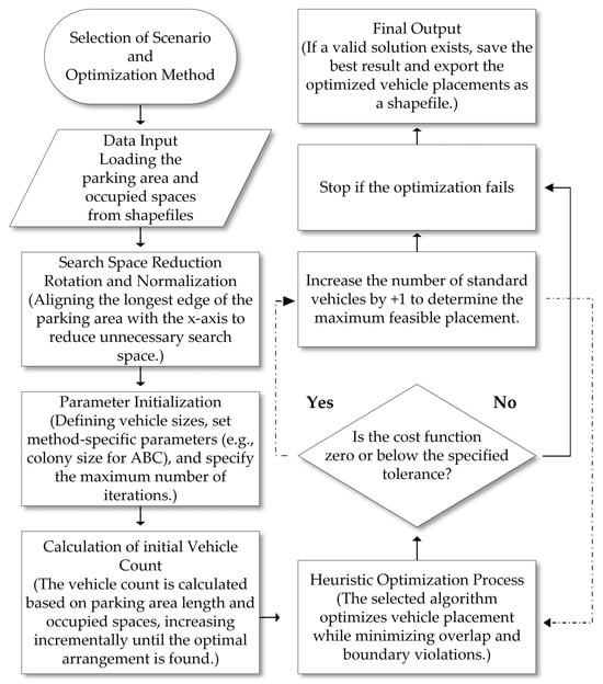
Figure 2.
Workflow of the optimization process (Source: author’s own elaboration).
As illustrated in Figure 2, following each successful optimization run, the number of vehicles is incremented by one (+1). This incremental approach is preferred over larger steps (e.g., +5) to minimize total computation time. Starting with a smaller number of vehicles allows the algorithm to quickly solve easier instances and avoid unnecessary time-consuming attempts for overly complex or infeasible configurations. This stepwise strategy ensures a more efficient search for the maximum feasible number of vehicles.
2.5. Heuristic Algorithms
Seven state-of-the-art heuristic algorithms were selected for comparative assessment:
- Particle Swarm Optimization (PSO);
- Phasor Particle Swarm Optimization (PPSO);
- Artificial Bee Colony (ABC);
- Gray Wolf Optimizer (GWO);
- Harris Hawks Optimization (HHO);
- Multi-Population Based Differential Evolution (MDE);
- Colony-Based Search Algorithm (CSA).
Their brief conceptual backgrounds, primary equations, and parameters are provided in the following subsections.
2.5.1. Particle Swarm Optimization (PSO)
PSO is a widely recognized optimization algorithm inspired by the collective behavior of natural systems, such as the synchronized movement of bird flocks and fish schools. First proposed by Kennedy and Eberhart [41], PSO has become a popular and effective method for solving complex optimization problems. As a stochastic, population-based optimization technique, it is particularly well-suited for addressing continuous optimization challenges.
The algorithm works by simulating a group of particles, each representing a potential solution within the problem space. These particles move through the solution space, interacting with one another to identify the best possible solution. Each particle updates its position and velocity based on two primary factors—its own best-known position (known as the cognitive component) and the best-known position of the entire swarm (referred to as the social component). The cognitive component guides the particle toward its personal best solution, while the social component encourages it to move toward the swarm’s global best solution. By combining these two influences, particles effectively balance individual exploration and collective knowledge, enabling them to converge toward optimal solutions [41].
At its core, PSO relies on an iterative process where particles continuously refine their positions and velocities based on their own experiences and the swarm’s collective performance. This process repeats until a predefined stopping condition, such as reaching a maximum number of iterations or achieving a satisfactory solution, is met. Thanks to its simplicity, efficiency, and adaptability, PSO has been successfully applied in various fields, including engineering, machine learning, and finance. However, the algorithm’s performance is highly sensitive to parameter settings, such as inertia weight and acceleration coefficients, which may need to be adjusted depending on the specific problem being solved [41].
The mathematical expressions of the PSO algorithm, including Equations (4)–(8), were adapted from [41]. The function to be optimized is denoted as , where represents the candidate solution vector, signifies the dimensionality of the vector, and stands for the iteration index. Each entity corresponds to a particular position within the search space. This relationship is expressed in Equation (4) [41].
The velocity and position of each entity are modified following the expressions given in Equations (5) and (6).
In these expressions, represents the inertia weight factor, and are the individual and collective learning coefficients, and are randomly generated values within the range , denotes the best-known position of entity , and represents the th component of the optimal position within the group [41].
To monitor the individual performance of each entity and determine the optimal solution within the group, the individual best position and the global best position are iteratively updated according to Equations (7) and (8) [41].
The optimization process in the PSO method can conclude when all entities converge to a common location, a predefined objective function threshold is met, or a specified number of iterations is completed.
2.5.2. Phasor Particle Swarm Optimization (PPSO)
PPSO, introduced by Ghasemi et al. [42], is a novel variant of the PSO algorithm designed to enhance performance, particularly for high-dimensional optimization problems. Inspired by phasor theory in mathematics, PPSO models the control parameters using a single phase angle, , for each particle, transforming the algorithm into a self-adaptive, trigonometric, balanced, and nonparametric meta-heuristic approach.
The mathematical expressions of the PPSO algorithm, including Equations (9) and (10), were adapted from [42]. In standard PSO, the velocity update relies on control parameters such as the inertia weight and acceleration coefficients and , which require careful tuning to balance exploration and exploitation. PPSO eliminates this need by incorporating these controls into periodic trigonometric functions, specifically and , where is the phase angle of particle at iteration. The phase angle is initialized randomly in the range and evolves over iterations, enabling adaptive search behaviors without explicit parameter adjustments [42].
The velocity update in PPSO is defined for each dimension as Equation (9) [42]:
Here, the functions and replace the traditional acceleration coefficients and , respectively. The inertia weight is set to zero in the basic PPSO formulation, simplifying the velocity update and emphasizing the influence of the personal best () and global best () positions. The position update remains consistent with standard PSO as Equation (10) [42]:
The phase angle is updated in each iteration to dynamically modulate the influence of the cognitive and social components. This adaptive mechanism effectively balances global exploration and local exploitation, reducing the risk of premature convergence to local optima, a common issue in standard PSO, especially in high-dimensional spaces. The optimization process iterates by updating particle positions and velocities based on the phase angle dynamics until a predefined stopping criterion is met, such as reaching a maximum number of iterations or achieving a sufficient fitness value for [42].
2.5.3. Artificial Bee Colony (ABC) Algorithm
The ABC algorithm, created by Karaboga [43], was designed to address numerical optimization issues by emulating the foraging behavior of honeybees. The perfect collaboration and systematic arrangement of bee colonies create the essential foundation for this algorithm. The ABC algorithm functions by simulating the actions of three categories of bees—employed bees, onlooker bees, and scout bees. Worker bees concentrate on particular food sources and communicate details about them, whereas observer bees choose food sources according to this communicated information. In contrast, scout bees are tasked with finding new sources of food. To streamline the process, half of the bees in the colony are regarded as employed bees, while the other half are observed bees. When a food supply is depleted, worker bees shift to the role of scout bees [43,44].
The ABC algorithm is recognized as a powerful technique for optimizing functions with multiple parameters. The way bees move according to the availability of food supplies allows the algorithm to provide an effective search method for solving problems. This method, which replicates the coordinated operation of natural bee colonies, offers a successful and novel solution for addressing intricate optimization challenges. The ABC algorithm involves three essential steps during each iteration: (1) deploying employed and onlooker bees to assess the quality of food sources, (2) deciding if scout bees will be released, and (3) guiding scout bees to new potential food sources if they emerge. In the model, the locations of the food sources signify possible solutions to the problem at hand, while the quantity of food at each source indicates the quality of these solutions. An increased quantity of food, signifying a superior solution, raises the likelihood of onlooker bees being drawn to that source. The quantity of scout bees is controlled by a “limit parameter”; if a food source does not show improvement after a specified number of attempts, the employed bee gives it up and turns into a scout bee. Throughout the solution development stage, a counter is utilized for each solution to monitor the number of unsuccessful attempts that indicate a lack of improvement [45,46].
The mathematical expressions of the ABC algorithm, including Equations (11)–(15), were adapted from [43,45,46]. In the initial phase, the algorithm generates a randomly distributed population of solutions using Equation (11).
Here, represents a candidate solution in the population. The index denotes the population size (), while represents the number of optimization parameters (). For each parameter, defines the lower boundary, whereas specifies the upper boundary. Candidate solutions are generated within these limits using randomly assigned values [45].
In the algorithm, the number of food sources is equal to the number of employed bees. Each employed bee stores the position of the source, its nectar amount, and the newly discovered sources in its memory. The bee identifies a new food source in its neighborhood using Equation (12), evaluates its quality, and if the new source is better, it forgets the previous one and memorizes the new location [45].
Each solution represents a food source, and is generated by modifying a single parameter of . This modification is based on a randomly selected neighbor , where the difference between their th parameters is weighted by a random factor in the range and added to . The parameter regulates the exploration around the current food source, ensuring diversity in solution search. If the generated exceeds the predefined parameter boundaries, it is adjusted to either the lower or upper limit using Equation (13), maintaining feasibility within the search space [45].
The new solutions generated by employed bees represent potential food sources. The quality of these sources is evaluated, and their fitness values are assigned using Equation (14).
Here represents the cost value of the solution . Employed bees perform a greedy selection between their current solutions and potential solutions based on fitness values. If is better, the bee replaces in its memory and resets the failure counter. Otherwise, it keeps and increases its failure counter by one. This process ensures efficient exploration and refinement of solutions [45].
When employed bees return to the hive, they share food source information through dances, which onlooker bees observe to assess nectar quality. Onlooker bees then select food sources based on probabilities calculated using Equation (15), where selection is proportional to nectar amount [45].
Here, represents the nectar amount (fitness) of the th source, and denotes the total number of food sources. After selecting a source, onlooker bees generate a candidate food source using Equation (12), similar to the employed bees search process. The new candidate is then compared with the existing solution . If the nectar amount of is greater than or equal to that of , the new source replaces the old one in memory; otherwise, the previous source is retained [45].
In the ABC algorithm, at the end of each cycle, both employed, and onlooker bees increment the failure counter for solutions that could not be improved. If an improvement occurs, the counter is reset to zero. Each solution has an associated failure counter, which increases if neither the employed nor the onlooker bee enhances it. When this counter exceeds a predefined threshold (limit parameter), the solution is considered depleted, and the employed bee abandons it. The bee then becomes a scout, generating a new random food source using Equation (11) to replace the exhausted one [45].
2.5.4. Harris Hawks Optimization (HHO)
Harris Hawks Optimization (HHO) is a population-based optimization algorithm inspired by the cooperative hunting behavior of Harris Hawks. Proposed by Heidari et al. [47], the method aims to achieve optimal solutions by emulating the natural hunting strategies of these hawks. HHO consists of two primary phases—the exploration phase, where hawks randomly search for prey or track the position of the best solution (the most optimal solution), and the exploitation phase, which refines the solution through various hunting strategies, including soft besiege, hard besiege, soft besiege with rapid dives, and hard besiege with rapid dives. Each hawk represents a solution in the search space, and the algorithm iteratively updates these solutions to converge toward the global optimum, striving to balance individual and collective behaviors to attain the optimal solution [47].
The mathematical expressions of the ABC algorithm, including Equations (16)–(27), were adapted from [47]. In HHO, the function to be optimized is defined, where represents the candidate solution vector, denotes the vector dimension, and is the iteration index. Equation (16) expresses the equality condition, where represents a solution at iteration , and the condition holds if the solution is feasible [47]:
During the exploration phase of the HHO algorithm, hawks randomly search for prey or orient themselves toward the position of the leader hawk (the best solution). The position update is governed by Equation (17) [47]:
Here, is a randomly selected hawk position, and are random numbers in the range , is a random parameter controlling the transition between the exploration and exploitation phases, is the average position of the population, and is a random scaling factor in the range [47].
In the exploitation phase, HHO employs various strategies based on the prey’s energy () and a random parameter . The prey’s energy, representing the movement capability of the prey, is calculated using Equation (18) [47]:
Here, is the randomly determined initial energy at each iteration, and is the maximum number of iterations. When , the exploration phase continues; when , the exploitation phase is employed. Four strategies are utilized in the exploitation phase: soft besiege, hard besiege, soft besiege with rapid dives, and hard besiege with rapid dives.
When the prey’s energy is high () and , the hawks softly encircle the prey in the soft besiege strategy. The position update is expressed by Equation (19) [47]:
Here, and , where is a random number representing the random jump strength of the prey.
Soft Besiege with Rapid Dives: When the prey’s energy is sufficiently high () and , the hawks adjust their positions based on the current strategy, utilizing the following formulations, as expressed by Equations (20) and (21) [47]:
If then ; otherwise, . Here, is a random vector, and , calculated using Equation (22), represents the Lévy flight vector [47]:
where , and are random numbers in the range , is the gamma function, and is a scaling factor.
Hard Besiege: When the prey’s energy is sufficiently low () and , the hawks encircle the prey more closely. This strategy is modeled using Equation (23) [47]:
Hard Besiege with Rapid Dives: When the prey’s energy is sufficiently low () and , the hawks adjust the population’s average position iteratively. This strategy is expressed by Equations (24) and (25) [47]:
If , then ; otherwise, .
The positions are updated iteratively using the best and global positions, as defined by Equations (26) and (27) [47]:
The HHO algorithm continues until the hawks reach a predefined threshold or the maximum iteration number () is achieved. The algorithm’s performance depends on the appropriate tuning of parameters , , and the Lévy flight parameters [47].
2.5.5. Gray Wolf Optimizer (GWO)
GWO is a metaheuristic algorithm based on population, drawing inspiration from the social organization and collaborative hunting practices of gray wolves (Canis lupus). Proposed by Mirjalili et al. [48], GWO has proven to be effective in addressing various intricate optimization issues in both continuous and discrete fields. The algorithm simulates the hierarchical structure of gray wolf packs, assigning individuals to four roles—alpha (), beta (), delta (), and omega (). The alpha wolves signify the most effective solutions discovered to date and direct the search operation, steering the remainder of the pack toward promising areas in the solution space. Beta and delta wolves enhance the optimization process by improving the search direction, whereas omega wolves concentrate on discovering different solutions. This organized framework maintains a productive equilibrium between exploration (looking for novel solutions) and exploitation (improving current solutions), boosting the algorithm’s effectiveness in finding optimal solutions [48,49].
At the heart of the GWO algorithm lies an iterative search mechanism, in which wolves adjust their locations continually by following the direction of the alpha, beta, and delta wolves. The surrounding mechanism enables wolves to modify their locations in relation to the optimal solutions recognized at every iteration, whereas the adaptive control parameter () manages the balance between exploration and exploitation. Through the integration of these mechanisms, GWO effectively explores the solution space, moving toward optimal solutions while reducing the likelihood of premature convergence [48].
Assuming that the total number of wolves is and the search domain has dimensions, the position of the th wolf can be represented as: . To mathematically model the hierarchical structure of the wolves, the most optimal solution is identified as the alpha () wolf. Consequently, the second and third most optimal solutions are classified as the beta () and delta () wolves, respectively. All remaining candidate solutions are considered as omega () wolves. Within the algorithm, the alpha wolf’s location corresponds to the estimated prey’s position [48].
The mathematical expressions of the GWO algorithm, including Equations (28)–(39), were adapted from [48]. The encircling behavior of gray wolves can be mathematically formulated as shown in Equations (28) and (29) [48].
Here, the set represents the current iteration, denotes the position vector of the prey, and corresponds to the position vector of a gray wolf. The set acts as a control coefficient, which is determined by the following Equation (30) [48].
Here, the set is a randomly generated variable within the range .The set represents the convergence factor, which is computed using the following Equations (31) and (32) [48]:
Here, the set is a randomly generated variable within the range . The set serves as a control coefficient, which linearly decreases from 2 to 0 over the course of iterations, as stated in Faris, Aljarah, Al-Betar, and Mirjalili [49], where and .
When gray wolves hunt their prey, the wolf initially guides the rest of the pack in encircling the prey. Subsequently, the wolf directs the and wolves to execute the capture. In the hierarchy of gray wolves, the , and wolves remain the closest to the prey; therefore, the estimated prey’s position is determined based on their locations. The corresponding mathematical model is formulated in Equations (33)–(39) as follows [48]:
The distance between and the , , and wolves is determined using Equations (33)–(39). Subsequently, the wolves adjust their positions to move towards the prey, as formulated in Equation (39).
The entire iterative process of GWO cycles through the steps of encircling, updating positions, and refining solutions until a predefined stopping criterion such as reaching a maximum number of iterations or achieving a satisfactory fitness value is met, thereby ensuring convergence toward the global optimum [48].
2.5.6. Multi-Population Based Differential Evolution (MDE) Algorithm
MDE, developed by Karkinli [50], is an iterative, population-based stochastic global optimization algorithm designed for both unimodal and multimodal problems. Unlike recursive methods, MDE is nonrecursive, enabling independent and parallel evolution of solution vectors. It does not require a parameter tuning phase and is capable of operating in both constrained and unconstrained search spaces.
MDE employs a unique mutation operator composed of elitist, random, and noise components. The elitist component enhances optimization performance in unimodal problems, while the random component maintains solution diversity in multimodal problems. Meanwhile, the noise component prevents premature convergence by preserving numerical diversity within the population [50].
The working mechanism of MDE can be conceptually compared to individuals temporarily leaving an imaginary sub-swarm to forage for better resources. These individuals, denoted as , explore more efficient food sources and then return to , sharing the discovered information with the rest of the population. During each iteration, the best vector is recalculated to reflect the newly acquired knowledge. The differences in foraging behavior among individuals are simulated using a crossover control matrix () and a scaling factor (), ensuring effective adaptation and exploration [50].
The mathematical expressions of the MDE algorithm, including Equations (40)–(53), were adapted from [50,51]. The population matrix of MDE, represented by , is defined based on the elements of , as formulated in Equation (40). Here, and denote the lower and upper search space boundaries for the th variable of the optimization problem . The objective function values for the vectors are computed using Equation (41). Here, represents all valid values (e.g., from 1 to 3 N) instead of a single , generalizing the notation to indicate that the algorithm processes all rows of the population matrix. Subsequently, the best global solution vector, denoted as , along with its corresponding objective function value, is determined using Equation (42) [50].
At the beginning of MDE’s iterative computation process, the vectors are randomly selected from the set using Equation (43). Here, is defined according to Equation (44). The permute function randomly shuffles the elements of the set according to the Discrete Uniform Distribution and returns the first elements of the reordered set as the output [50].
The general system equation of MDE is given in Equation (45). In this equation, , , , and represent the trial vectors, crossover control matrix, temporary vectors, and noise values, respectively. The noise component prevents numerical entropy degradation in the trial vectors. The map matrix, which governs the crossover operation, is generated using Equation (46). The vector, representing the th variable of the th temporary vector, is calculated using Equation (47). Finally, the scaling variable is obtained using Equation (48) [50].
The scaling strategy of MDE can generate exponential values, enabling the algorithm to escape local optima and produce trial vectors () that guide the search towards more effective solutions. The noise vectors are computed as shown in Equation (49) where is Hadamard multiplication operator [50].
MDE evolves the trial vectors using the vectors. Equation (50) ensures that the parameters remain within the search boundaries. Equation (51) is used to update the matrix and values based on the fitness of the trial vectors [50].
At the end of each iteration, MDE updates the population and the global best solution. This process is described in Equations (52) and (53) [50].
2.5.7. The Colony-Based Search Algorithm (CSA)
The CSA is a novel evolutionary computation method developed by Civicioglu and Besdok [52] in 2024 to solve numerical optimization problems. This algorithm aims to provide a more effective search process by utilizing different mutation and crossover strategies. In evolutionary algorithms, the ability to maintain diversity within the population is a decisive factor in overall performance. CSA addresses this issue by employing a specialized mechanism that can preserve the numerical diversity of the population over extended periods. The algorithm creates a Clan Matrix containing pattern vectors randomly selected from the Colony Matrix in each iteration, thereby ensuring the preservation of numerical differences among solutions [52].
One of the most notable features of CSA is its use of a multi-component mutation strategy. This method generates new solutions through the random combination of three distinct components with different characteristics. Additionally, the algorithm employs an efficient approach for scaling the guidance vector, optimizing the direction of numerical evolution. Unlike common methods, such as standard differential evolution (DE) and particle swarm optimization (PSO), CSA updates the guidance vectors based on a bijective evolutionary search direction. As a result, each pattern vector evolves toward another pattern vector, enabling the algorithm to explore a broader search space [52].
The mathematical expressions of the CSA, including Equations (54)–(63), were adapted from [52]. The main population of the CSA is referred to as the Colony Matrix (), which comprises a randomly initialized solution vector of size , corresponding to times the size of the Clan Matrix (). The initial Colony Matrix () and the objective function values of the colony patterns () are generated using the procedure described in Equation (54). Here, denotes the dimension of the problem, represents the objective function, while define the lower and upper boundaries of the search space, respectively [52].
The generation process of the swarm clan, and the objective function values of the patterns in are expressed Equation (55). Here, represents a random permutation function that selects elements from the initial colony.
The scale factor () used in the CSA to regulate the amplitude of the direction vector is computed using Equation (56). Here , follows a Lévy distribution, and denotes the scaling vector and Hadamard division operator, respectively. The function in Equation (57) generates a new real number from a uniform distribution at each call. Therefore, the two calls in the expression are independent of each other [52].
Lévy flights introduce the necessary exploration capability to escape local optima and discover diverse, high-quality solutions within complex search spaces. By enabling occasional long jumps, Lévy flights improve global search efficiency, increasing robustness and preventing the algorithm from becoming trapped. The Lévy distribution is a probability distribution characterized by heavy tails, which means it has a higher likelihood of generating extreme values compared to a normal distribution [52]. The probability density function (PDF) of the Lévy distribution is defined in Equation (58). Here, is the random variable, represents the location parameter, and denotes the scale parameter of the distribution.
The binary-valued mutation control matrix () in CSA is generated using the procedure outlined in Equation (59). Here, “” represents the piecewise power operator used in the mutation mechanism to introduce randomness and preserve diversity in the population. The function generates a new random integer-valued matrix with rows and 1 column at each call. The generated values are uniformly distributed over the interval [52].
The CSA utilizes Equation (60) to generate the evolutionary direction (), which is responsible for guiding the search process in the solution space. Here, are randomly selected indices using the randperm function, ensuring diverse exploration by introducing different solution perturbations [52].
The morphogenesis matrix, which governs the offspring patterns in the CSA, is generated using Equation (61). This equation integrates directional evolution (), scaling factors (), and morphological adjustments (), ensuring structured yet diverse exploration in the search space [52].
In the final phase of each iteration, the CSA updates the colony patterns by incorporating the patterns from the clan, as formulated in Equation (62).
At the end of the current iteration, the numerical value of the best solution is updated using Equation (63), ensuring that the algorithm retains the optimal solution discovered so far [52].
3. Results and Discussion
In this section, the performance of the ABC, CSA, GWO, HHO, MDE, PSO, and PPSO algorithms is evaluated across three different parking optimization scenarios. These scenarios represent increasing levels of complexity based on the rotational freedom of vehicles within the parking area. The evaluation criteria include the maximum number of parked vehicles, computation time, and solution consistency.
The findings are based on simulation results conducted using real-world parking areas in Kayseri. Each method and scenario was executed 30 times, and the results illustrate performance across repeated trials.
The performance outcomes of the implementations are presented in Table 2, Table 3, Table 4 and Table 5. Additionally, a graphical comparison of the results for each method is provided in Figure 3. Table 2 presents the number of runs (out of 30) in which each algorithm achieved its maximum number of successfully placed vehicles. The optimization process for each algorithm begins with a low vehicle count and incrementally increases the number until no valid solution can be found. As such, the values in the table indicate how often an algorithm terminated at a specific vehicle count as its best result. Since some algorithms failed to find feasible solutions in certain runs, the total number of successful results is less than 30. For example, ABC, GWO, HHO, and PPSO achieved valid placements in only a limited number of runs due to the complexity of the scenarios.
Table 2.
Frequency table for the maximum number of successfully placed vehicles over 30 runs for each algorithm (source: author’s own elaboration).
Table 3.
Maximum number of successfully placed vehicles, mean solution time, and cumulative maximization time (source: author’s own elaboration).
Table 4.
Mean computation time (in seconds) per trial for each vehicle count in placement optimization (source: author’s own elaboration).
Table 5.
Success rate distribution over 30 runs (source: author’s own elaboration).
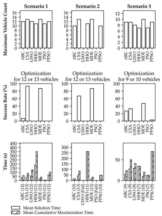
Figure 3.
Performance comparison of optimization methods (source: author’s own elaboration).
In Table 3 and Table 4, the mean solution time refers to the average computation time required by each algorithm to successfully place a specific number of vehicles over 30 independent runs. The mean cumulative maximization time represents the average total time taken by the algorithm throughout the incremental optimization process, in which the number of vehicles is gradually increased until no feasible solution can be found. This metric provides insight into the overall computational cost of reaching the optimal placement result.
3.1. Results of Scenario 1: Parallel Parking Without Rotation on Parking Area 1
In this scenario, vehicles were parked in a parallel manner without any rotational freedom. According to the data in Table 1 and Table 2, MDE and the CSA achieved the best results from the perspective of the adopted objective function by placing a maximum of 13 vehicles. ABC, GWO, and PPSO managed to place up to 12 vehicles, while HHO and PSO reached a maximum of 11.
According to Table 3, the MDE algorithm provided the fastest solution, placing 13 vehicles in an average of 19.21 s. In contrast, the CSA achieved the same result in approximately 36.68 s, making it nearly twice as slow as MDE. Notably, MDE demonstrated high consistency, reaching maximum capacity in approximately 50% of the trials, making it the most reliable algorithm in this scenario.
In cumulative trials for achieving maximum capacity, MDE required 40.68 s, while the CSA took 86.06 s. Since placing 13 vehicles is more challenging than 12 vehicles, the success rates presented in Table 4 are crucial. The CSA achieved a 93.3% success rate in placing 12 or 13 vehicles, while MDE had a 90% success rate. However, MDE successfully placed 13 vehicles in 50% of trials, whereas the CSA achieved this only 20% of the time. Therefore, MDE was identified as the best optimization method for Scenario 1.
In conclusion, MDE and CSA were the most robust and consistent methods for this type of application. The other algorithms exhibited lower performance in comparison. Additionally, ABC outperformed GWO, HHO, PSO, and PPSO, demonstrating better optimization capabilities. PPSO also yielded better results than GWO, HHO, and PSO in terms of both vehicle placement and success rates, although it remained less competitive than ABC, the CSA, and MDE.
3.2. Results of Scenario 2: Parking with Rotation Optimization up to 45 Degrees on Parking Area 1
In this scenario, vehicle rotations were optimized, allowing a maximum rotation of up to 45 degrees. According to Table 1 and Table 2, MDE and the CSA achieved the best results, successfully placing a maximum of 13 vehicles. ABC and PPSO placed up to 10 vehicles, while PSO and GWO failed to produce valid solutions. HHO was able to place a maximum of 11 vehicles.
As shown in Table 3, the MDE algorithm provided the fastest solution, placing 13 vehicles in an average of 13.05 s. Meanwhile, the CSA took 42.21, and HHO required 260.72 s to place 11 vehicles, indicating a significant performance gap. The cumulative maximization time for MDE was 29.82 s, whereas the CSA required 85.63 s. PPSO’s total time for placing 10 vehicles was 46.18 s.
Compared to Scenario 1, this scenario introduced additional complexity due to the inclusion of angle optimization, increasing the number of parameters to be optimized. This increased complexity resulted in longer computation times and reduced success rates for most algorithms except MDE. Surprisingly, MDE performed even better in this scenario, demonstrating how different optimization methods can yield varying results under different conditions.
According to Table 5, MDE achieved an 87% success rate in placing 12 or 13 vehicles, making it the most reliable algorithm. The CSA followed with 67%. MDE successfully placed 13 vehicles in 43% of trials, compared to 10% for the CSA. Other methods, including PPSO and HHO, performed better than GWO and PSO but remained notably less competitive than MDE and the CSA.
These results indicate that MDE is the most effective algorithm in terms of both speed and success rate. While the CSA demonstrated competitive performance under certain conditions, MDE was selected as the best optimization method for Scenario 2 due to its superior placement efficiency and stability.
Overall, allowing rotation up to 45 degrees enabled a higher number of vehicles to be placed in the parking area. However, this optimization also posed challenges for some algorithms, with ABC, GWO, HHO, PSO, and PPSO performing worse compared to MDE and CSA.
3.3. Results of Scenario 3: Parking with Full Rotation Optimization (0–180 Degrees) on Parking Area 2
In this scenario, vehicle rotations were fully optimized, allowing rotation between 0 and 180 degrees. Providing full angular flexibility in a perpendicular parking area increased the complexity of the problem and posed additional optimization challenges. According to Table 1 and Table 2, the MDE algorithm achieved the best performance, successfully placing a maximum of 10 vehicles, while the CSA, ABC, and PPSO placed up to 9 vehicles. GWO managed to place 8 vehicles, while PSO and HHO exhibited the lowest performance in this scenario.
According to Table 3, the MDE algorithm provided the fastest solution, placing 10 vehicles in an average of 9.65 s. The ABC (14.91 s), CSA (27.88 s), and PPSO (69.63 s) algorithms required significantly more time, while GWO (29.15 s), HHO (34.22 s), and PSO (12.66 s) exhibited lower efficiency. In terms of cumulative maximization time, MDE achieved the best efficiency with a total computation time of 19.92 s, while CSA and ABC required 50.10 and 23.55 s, respectively.
The inclusion of full angular optimization significantly increased the number of parameters to be optimized, making the problem more complex. This complexity negatively affected the performance of some algorithms, leading to longer computation times and reduced success rates. However, MDE successfully reached maximum capacity in the shortest time despite these challenges. Notably, ABC performed better in this scenario compared to previous ones, suggesting that it is more effective when angular flexibility is introduced. This improvement may be attributed to ABC’s strong exploration capability and ability to efficiently navigate a larger search space. Similarly, PPSO outperformed GWO, PSO, and HHO in terms of vehicle count, suggesting its relative effectiveness under high-complexity conditions. These findings highlight the varying performance of different optimization methods when applied to complex problems.
As shown in Table 5, MDE achieved a 47% success rate in placing 9 or 10 vehicles, making it the most reliable algorithm. CSA and ABC followed with success rates of 33% and 27%, respectively. However, MDE managed to place 10 vehicles in only 3% of the trials, while CSA and ABC failed to achieve this in any trial. Based on these results, MDE was identified as the best optimization method for Scenario 3.
Overall, allowing full angular optimization enabled higher vehicle placement capacity, but the added flexibility also made the problem significantly more challenging. CSA, ABC, and PPSO produced relatively successful results under specific conditions, but MDE once again demonstrated the best performance. GWO, HHO, and PSO exhibited lower success rates and longer computation times compared to the other methods.
3.4. Evaluation of Different Vehicle Types and Parking Areas
Figure 4 presents the best vehicle placement configurations achieved by each method across different scenarios. In Scenario 1, the ABC method utilized the small remaining space at the end of the parking area by placing a Citroën AMI, while the CSA method attempted to fit a standard vehicle within this space by pushing the cost function tolerance limits. Since ABC, GWO, HHO, PSO, and PPSO placed fewer vehicles, they resulted in a more flexible parking arrangement. In contrast, MDE successfully accommodated 13 vehicles. If the small remaining space at the end of the parking area had been used, a second AMI could have increased the total vehicle count to 14. However, to ensure a standard comparison across all methods, only one AMI and one Crafter were included in each scenario. Scenario 1 demonstrated that the Volkswagen Crafter did not pose significant challenges, while Figure 4 highlights the importance of developing flexible solutions for unmarked parking areas.
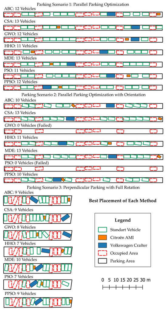
Figure 4.
Best parking arrangements achieved by each optimization method (source: author’s own elaboration).
According to Figure 4, in Scenario 2, only ABC, CSA, MDE, HHO, and PPSO produced optimal parking arrangements. GWO and PSO failed to generate any feasible solutions within the maximum iteration limit. HHO managed to place 11 vehicles, performing better than ABC and PPSO in terms of capacity, though its layout was more constrained. ABC and PPSO placed two fewer vehicles compared to the CSA and MDE, resulting in a more flexible layout. The CSA, despite maximizing the number of parked vehicles, utilized the tolerance limits, leading to two adjacent vehicles touching each other. Meanwhile, MDE placed the vehicles in a more balanced manner than the CSA. Additionally, both MDE and the CSA positioned the Citroën AMI in the remaining space at the end of the parking area due to its compact dimensions.
For Scenario 3, Figure 4 indicates that the Volkswagen Crafter was the most challenging vehicle to park. As its length exceeded the perpendicular width of the parking area, it had to be rotated, making it a more complex optimization problem. In this scenario, MDE achieved the highest vehicle placement count with 10 vehicles, but the Crafter’s placement remained highly challenging. ABC, the CSA, and PPSO placed up to 9 vehicles, while GWO, PSO, and HHO placed fewer. Although GWO, the CSA, and ABC placed fewer vehicles, they provided relatively more feasible parking arrangements for the Volkswagen Crafter. As seen in Figure 4, while MDE managed to fit 10 vehicles, it resulted in a more constrained parking scenario for the Crafter. PSO and HHO placed only 7 vehicles but still failed to provide a more spacious arrangement. When comparing different methods, ABC, the CSA, and GWO produced more accessible parking layouts, which facilitated easier entry and exit. Although MDE achieved the highest vehicle capacity, it did so by minimizing the space between Citroën AMI and Volkswagen Crafter, utilizing the cost function’s tolerance limits. It is suggested that MDE’s performance could be further improved by reducing the tolerance threshold, allowing for a more precise solution. Alternatively, MDE could be adjusted to place fewer vehicles, avoiding excessive space constraints.
Unmarked parking areas are not limited to roadside parking; they are also commonly used in temporary market areas, concert venues, and large open spaces. The proposed optimization framework can be applied to such large parking areas. In these cases, the parking area can be divided into predefined blocks, enabling the framework presented in this study to be executed simultaneously or separately for each block. Figure 5 provides a conceptual representation of the block-based approach for large parking areas.
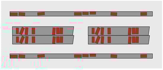
Figure 5.
Example of block division for optimization in large parking areas (source: author’s own elaboration).
3.5. Discussion
The methods and scenarios examined in this study reveal how optimization performance varies under different conditions. While the study by Janowski, Hüsrevoğlu, and Renigier-Bilozor [31] used only the ABC algorithm, which provided satisfactory results for the given problem, the CSA and MDE methods achieved significantly better outcomes as the complexity of the problem increased. Across all three scenarios, MDE consistently delivered the best performance both in terms of maximum vehicle placement and computational speed. The CSA followed MDE as the second most successful method overall, demonstrating strong and stable performance, particularly in Scenarios 1 and 2. PPSO also performed better than PSO in all tested scenarios, indicating the advantage of this modern variant. ABC demonstrated stable performance in simpler scenarios and outperformed GWO, HHO, PSO, and PPSO in terms of vehicle placement frequency and success rates. However, HHO was able to surpass ABC in Scenario 2 in terms of maximum vehicle count, despite its longer computation time.
The MDE algorithm demonstrated clear superiority over other methods in terms of both computation time and robustness across all scenarios, positioning it as a strong candidate for future research on similar problems. Additionally, MDE and the CSA, which yielded successful results in this study, require minimal parameter tuning, apart from setting the population size and iteration count. One of the key findings of this study is that such complex optimization problems can be solved efficiently and that the choice of method plays a crucial role in both solution time and accuracy, as supported by previous research on machine learning model calibration [53].
Apart from their effectiveness and ease of implementation, the underlying structures of MDE and the CSA also offer practical advantages in terms of computational efficiency. PSO and GWO are semi-parallel algorithms in which individual particle or wolf updates can be computed concurrently, though the update of the leader information requires synchronization. In contrast, MDE’s multi-population structure is inherently more suitable for parallel computation, and the CSA offers similar advantages. Considering that MDE achieves superior performance in a short period, its efficiency could be further optimized through advanced parallel programming techniques.
Furthermore, the improved performance of PPSO compared to PSO suggests that algorithmic refinements can significantly enhance optimization capabilities. PPSO’s phase-based dynamics enabled better convergence behavior, particularly in scenarios where precise spatial coordination was required. These findings underscore the value of employing enhanced or hybrid versions of established methods in similar applications.
This research makes a significant contribution to the literature by addressing how to maximize the utilization of available space in unmarked parking areas. By utilizing the Janowski, Hüsrevoğlu, and Renigier-Bilozor [31] framework, a comparative analysis of different vehicle types, parking area types, and optimization methods was conducted. As one of the few studies focused on this problem, this work provides a new perspective on vehicle placement optimization.
In addition to maximizing capacity, several other factors should be considered to enhance the applicability and reliability of the system. For instance, in sloped environments, placing vehicles perpendicular to the direction of the incline may lead to safety concerns, reduced stability, or maneuvering difficulties. Assigning preferred or constrained rotation angles based on local terrain slope could improve both safety and spatial feasibility. This information could be derived automatically from external geospatial sources such as digital elevation models or three-dimensional point clouds or entered manually if unavailable.
Building on this, future research could benefit from adopting a multi-objective optimization approach that reflects the complex trade-offs encountered in realistic parking scenarios. Beyond maximizing vehicle count, relevant objectives may include minimizing entrance and exit conflicts, reducing computation time, aligning vehicle orientation with slope or signage, minimizing the distance to zone entry points, and avoiding overlaps in maneuvering paths. These competing goals may be handled using various optimization strategies, such as scalarization techniques with weighted preferences [54], indicator-based evolutionary algorithms that prioritize solution quality metrics, or decomposition-based frameworks like the MOEA/D (the Multi-Objective Evolutionary Algorithm Based on Decomposition) [55]. Incorporating these methods could significantly improve the flexibility, robustness, and user-centered applicability of the proposed system.
For future studies, implementing the proposed framework in real-world applications requires segmenting vehicles within the parking area and transmitting their geometric data to the optimization algorithm via a server, as in the study by Janowski, Hüsrevoğlu, and Renigier-Bilozor [31]. In real-world scenarios, when a vehicle exits or a new vehicle enters the parking area, it is crucial to rapidly determine new optimal placements.
When analyzing the solution times of the MDE algorithm, the results indicate that in Scenario 1 (parallel parking), the placement of 10 to 13 vehicles required between 3.65 and 19.21 s. In Scenario 2 (limited angular freedom), the optimization process was completed within 3 to 13.05 s, while in Scenario 3 (full angular freedom), the computation time ranged from 1.94 to 9.65 s. Notably, the maximum computation times in Scenario 2 (13.05 sec) and Scenario 3 (9.65 sec) suggest that these methods could be feasible for real-time applications. These durations reflect full-capacity optimization, representing the time required to place between 10 and 13 vehicles. In typical real-time scenarios involving smaller changes, such as the arrival or departure of 1 to 5 vehicles, the computation time may be significantly shorter. In practical cases with fewer available parking spaces, the solution space would be smaller, leading to even faster computation times. Additionally, by narrowing the solution space, such as limiting rotation angles or adjusting algorithm parameters, the problem can be simplified for less complex settings, further accelerating the process. However, further reductions in computation time would be beneficial for future implementations.
Since the literature includes numerous optimization methods, it is recommended that alternative approaches be investigated for this purpose. As illustrated in Figure 5, even though vehicles were optimally placed according to predefined constraints, additional restrictions may be required to enhance entry and exit convenience. In this regard, future studies should focus on both reducing optimization time and improving vehicle maneuverability, potentially through advanced constraint handling and additional optimization strategies. Future studies may also consider incorporating additional objectives such as reducing the carbon footprint, shortening parking duration, and facilitating easier entry and exit.
4. Conclusions
In modern urban life, the efficient utilization of unmarked parking areas is as crucial as the solutions developed for marked parking spaces. This study has demonstrated optimization approaches that maximize vehicle capacity by effectively utilizing the available space in unmarked parking areas. The analyses conducted using different vehicle types and parking scenarios have clearly highlighted the performance differences among various optimization methods.
The findings of this study lay the foundation for a system that could be integrated into future smart city applications. In such a system, users would be able to view available parking spaces suitable for their vehicle dimensions in real-time through a spatial application and be guided to the most optimal parking locations. For instance, large vehicles such as the Volkswagen Crafter, a long panel van, could be directed to wider spaces or areas where they can park at specific angles, while the Citroën AMI or standard-sized vehicles could be guided to narrower and more optimized spaces. By offering parking solutions tailored to different vehicle types, the available space could be utilized with maximum efficiency.
This approach not only enhances individual convenience but also reduces traffic congestion caused by parking searches, lowers unnecessary fuel consumption, and significantly contributes to environmental sustainability. Moreover, it can prevent large vehicles from parking in inappropriate locations, making space utilization more efficient and enabling the development of smart parking management systems that save drivers time.
Furthermore, unmarked parking areas in temporary market zones or fairgrounds could particularly benefit from the proposed block-based optimization framework. Future studies may explore the applicability of this method in dynamic and irregular settings such as open-air bazaars, where rapid and flexible space optimization is essential due to temporal and spatial constraints. This study makes a significant contribution to the literature on the optimization of unmarked parking areas while also opening new avenues for future research. Advanced smart systems could further accelerate optimization processes, providing real-time solutions and integrating them into urban transportation planning. As a result, beyond individual benefits, this approach could support the development of smarter and more sustainable parking management strategies at the city-wide level, contributing to urban planning and mobility solutions.
Author Contributions
Conceptualization, M.H., A.J. and A.E.K.; methodology, M.H., A.J. and A.E.K.; software, M.H., A.J. and A.E.K.; validation, M.H., A.J. and A.E.K.; formal analysis, M.H., A.J. and A.E.K.; investigation, M.H., A.J. and A.E.K.; resources, M.H., A.J. and A.E.K.; data curation, M.H., A.J. and A.E.K.; writing—original draft preparation, M.H., A.J. and A.E.K.; writing—review and editing, M.H., A.J. and A.E.K.; visualization, M.H., A.J. and A.E.K.; supervision, M.H., A.J. and A.E.K.; project administration, M.H., A.J. and A.E.K.; funding acquisition, M.H., A.J. and A.E.K. All authors have read and agreed to the published version of the manuscript.
Funding
This research received no external funding.
Institutional Review Board Statement
Not applicable.
Informed Consent Statement
Not applicable.
Data Availability Statement
Publicly available datasets were analyzed in this study. This data can be found here: https://github.com/Aekarkinli/Metaheuristic-Optimizing-Vehicle-Placement (accessed on 29 May 2025).
Conflicts of Interest
The authors declare no conflicts of interest.
References
- Zhou, C.; Petryshyn, H.; Liubytskyi, R.; Kochan, O. Optimization of on-street parking in the historical heritage part of Lviv (Ukraine) as a prerequisite for designing the IoT smart parking system. Buildings 2022, 12, 865. [Google Scholar] [CrossRef]
- Plasencia-Lozano, P.; Méndez-Manjón, I. Optimisation of urban space based on geometric analysis of parallel parking lots. Transp. Res. Procedia 2023, 71, 307–314. [Google Scholar] [CrossRef]
- Dey, S.S.; Dance, C.R.; Darst, M.; Dock, S.; Silander, T.; Pochowski, A. To demarcate or not to demarcate: Analysis of marked versus unmarked on-street parking efficiency. Transp. Res. Rec. 2016, 2562, 18–27. [Google Scholar] [CrossRef]
- Ismael, A.; Holguín-Veras, J. Optimal parking allocation for heterogeneous vehicle types. Transp. Res. Part A Policy Pract. 2025, 192, 104357. [Google Scholar] [CrossRef]
- Xu, C.; Skiena, S. Marking streets to improve parking density. arXiv 2015, arXiv:1503.09057. [Google Scholar]
- Xu, T. Simulation study of the efficiency of unmarked on-street parking and vehicle downsizing. Transp. Res. Rec. 2019, 2673, 367–376. [Google Scholar] [CrossRef]
- Bazzi, A.; Slock, D.T.; Meilhac, L. Online angle of arrival estimation in the presence of mutual coupling. In Proceedings of the 2016 IEEE Statistical Signal Processing Workshop (SSP), Palma de Mallorca, Spain, 26–29 June 2016; pp. 1–4. [Google Scholar]
- Chen, Y.; Wang, T.; Yan, X.; Wang, C. An ensemble optimization strategy for dynamic parking-space allocation. IEEE Intell. Transp. Syst. Mag. 2022, 15, 347–362. [Google Scholar] [CrossRef]
- Bai, Y.; Qian, Q. Optimal placement of parking of electric vehicles in smart grids, considering their active capacity. Electr. Power Syst. Res. 2023, 220, 109238. [Google Scholar] [CrossRef]
- Duan, F.; Eslami, M.; Khajehzadeh, M.; Alkhayer, A.G.; Palani, S. An improved meta-heuristic method for optimal optimization of electric parking lots in distribution network. Sci. Rep. 2024, 14, 20363. [Google Scholar] [CrossRef]
- Jamaludin, M.H.B.; Zhou, Y.; Yeoh, J.K. Automated basement car park design: Impact of design factors on static capacity. J. Archit. Eng. 2024, 30, 04024013. [Google Scholar] [CrossRef]
- Dong, N.; Fang, X.; Wu, A.-g. A novel chaotic particle swarm optimization algorithm for parking space guidance. Math. Probl. Eng. 2016, 2016, 5126808. [Google Scholar] [CrossRef]
- Carrese, S.; d’Andreagiovanni, F.; Giacchetti, T.; Nardin, A.; Zamberlan, L. An optimization model for renting public parking slots to carsharing services. Transp. Res. Procedia 2020, 45, 499–506. [Google Scholar] [CrossRef]
- Carrese, S.; d’Andreagiovanni, F.; Giacchetti, T.; Nardin, A.; Zamberlan, L. An optimization model and genetic-based matheuristic for parking slot rent optimization to carsharing. Res. Transp. Econ. 2021, 85, 100962. [Google Scholar] [CrossRef]
- Sayarshad, H. Designing intelligent public parking locations for autonomous vehicles. Expert Syst. Appl. 2023, 222, 119810. [Google Scholar] [CrossRef]
- Singh, R.; Dutta, C.; Singhal, N.; Choudhury, T. An improved vehicle parking mechanism to reduce parking space searching time using firefly algorithm and feed forward back propagation method. Procedia Comput. Sci. 2020, 167, 952–961. [Google Scholar] [CrossRef]
- Çakıcı, Z.; Şensoy, A.T. Determining the optimum parking angles for various rectangular-shaped parking areas: A particle swarm optimization-based model. Konya J. Eng. Sci. 2023, 11, 1016–1034. [Google Scholar] [CrossRef]
- Channamallu, S.S.; Kermanshachi, S.; Rosenberger, J.M.; Pamidimukkala, A. Smart parking systems: A comprehensive review of digitalization of parking services. Green Energy Intell. Transp. 2025, 100293. [Google Scholar] [CrossRef]
- Singh, T.; Khan, S.S.; Chadokar, S. A Review on Automatic Parking Space Occupancy Detection. In Proceedings of the International Conference on Advanced Computation and Telecommunication (ICACAT), Bhopal, India, 28–29 December 2018; pp. 1–5. [Google Scholar]
- Alam, M.; Moroni, D.; Pieri, G.; Tampucci, M.; Gomes, M.; Fonseca, J.; Ferreira, J.; Leone, G.R. Real-time smart parking systems integration in distributed its for smart cities. J. Adv. Transp. 2018, 2018, 1485652. [Google Scholar] [CrossRef]
- Chen, M.; Chang, T. A Parking Guidance and Information System Based on Wireless Sensor Network. In Proceedings of the IEEE international conference on information and automation, Shanghai, China, 10–12 June 2011; pp. 601–605. [Google Scholar]
- Sifuentes, E.; Casas, O.; Pallas-Areny, R. Wireless magnetic sensor node for vehicle detection with optical wake-up. IEEE Sens. J. 2011, 11, 1669–1676. [Google Scholar] [CrossRef]
- Gong, J.; Raut, A.; Pelzer, M.; Huening, F. Marking-based perpendicular parking slot detection algorithm using LiDAR sensors. Vehicles 2024, 6, 1717–1729. [Google Scholar] [CrossRef]
- Li, W.; Cao, L.; Yan, L.; Li, C.; Feng, X.; Zhao, P. Vacant parking slot detection in the around view image based on deep learning. Sensors 2020, 20, 2138. [Google Scholar] [CrossRef]
- Zinelli, A.; Musto, L.; Pizzati, F. A Deep-Learning Approach for Parking Slot Detection on Surround-View Images. In Proceedings of the IEEE Intelligent Vehicles Symposium (IV), Paris, France, 9–12 June 2019; pp. 683–688. [Google Scholar]
- Thakur, N.; Bhattacharjee, E.; Jain, R.; Acharya, B.; Hu, Y.-C. Deep Learning-Based Parking Occupancy Detection Framework Using ResNet and VGG-16. Multimed. Tools Appl. 2024, 83, 1941–1964. [Google Scholar] [CrossRef]
- Sairam, B.; Agrawal, A.; Krishna, G.; Sahu, S.P. Automated Vehicle Parking Slot Detection System Using Deep Learning. In Proceedings of the Fourth International Conference on Computing Methodologies And Communication (ICCMC), Erode, India, 11–13 March 2020; pp. 750–755. [Google Scholar]
- Grbić, R.; Koch, B. Automatic vision-based parking slot detection and occupancy classification. Expert Syst. Appl. 2023, 225, 120147. [Google Scholar] [CrossRef]
- Matsuda, A.; Matsui, T.; Matsuda, Y.; Suwa, H.; Yasumoto, K. A method for detecting street parking using dashboard camera videos. Sens. Mater. 2021, 33, 17. [Google Scholar] [CrossRef]
- Rafique, S.; Gul, S.; Jan, K.; Khan, G.M. Optimized real-time parking management framework using deep learning. Expert Syst. Appl. 2023, 220, 119686. [Google Scholar] [CrossRef]
- Janowski, A.; Hüsrevoğlu, M.; Renigier-Bilozor, M. Sustainable parking space management using machine learning and swarm theory—The SPARK system. Appl. Sci. 2024, 14, 12076. [Google Scholar] [CrossRef]
- ISPARK. Istanbul Metropolitan Municipality ISPARK. Available online: https://ispark.istanbul/ (accessed on 10 March 2025).
- Deniz, M.E. IstPark. Available online: https://apps.apple.com/tr/app/i-stpark/id1667266907?l (accessed on 10 March 2025).
- SONAH. Your Parking Management Solution. Available online: https://www.sonah.tech/parking-management (accessed on 7 March 2025).
- Grover, R.; Walacik, M. Property valuation and taxation for fiscal sustainability–lessons for Poland. Real Estate Manag. Valuat. 2019, 27, 35–48. [Google Scholar] [CrossRef]
- Chmielewska, A.; Walacik, M.; Grover, R. Property valuation principles—How policy changes can be detrimental to urban development. Land Use Policy 2025, 150, 107474. [Google Scholar] [CrossRef]
- Citroën. Citroën AMI Onboard Documentation. Available online: https://www.citroen.co.uk/content/dam/citroen/uk/b2c/tools/brochure/pdf/accesories/AMI_brochure.pdf (accessed on 7 March 2025).
- Volkswagen Commercial Vehicles. The Crafter Panel van Brochure. Available online: https://www.volkswagen-vans.co.uk/idhub/content/dam/onehub_nfz/importers/gb/downloads/brochures/crafter/crafter_panel_van-brochure.pdf (accessed on 7 March 2025).
- The Institution of Structural Engineers. Design Recommendations for Multi-Storey and Underground Car Parks, 4th ed.; The Institution of Structural Engineers: London, UK, 2011; pp. 1–98. [Google Scholar]
- Istanbul Metropolitan Municipality. İstanbul Büyükşehir Belediyesi Otopark Yönetmeliği (Istanbul Metropolitan Municipality Parking Regulation); Istanbul Metropolitan Municipality: Istanbul, Türkiye, 2006.
- Kennedy, J.; Eberhart, R. Particle Swarm Optimization. In Proceedings of the ICNN’95-International Conference On Neural Networks, Perth, WA, Australia, 27 November–1 December 1995; pp. 1942–1948. [Google Scholar]
- Ghasemi, M.; Akbari, E.; Rahimnejad, A.; Razavi, S.E.; Ghavidel, S.; Li, L. Phasor particle swarm optimization: A simple and efficient variant of PSO. Soft Comput. 2019, 23, 9701–9718. [Google Scholar] [CrossRef]
- Karaboga, D. An Idea Based on Honey Bee Swarm for Numerical Optimization: Technical Report-Tr06; Erciyes University, Engineering Faculty, Computer Engineering Department: Kayseri, Turkey, 2005; pp. 1–10. [Google Scholar]
- Karaboga, D.; Akay, B. A comparative study of artificial bee colony algorithm. Appl. Math. Comput. 2009, 214, 108–132. [Google Scholar] [CrossRef]
- Karaboga, D. Yapay Zekâ Optimizasyon Algoritmaları, 6th ed.; Nobel Akademi Yayınları: Ankara, Türkiye, 2018. [Google Scholar]
- Karaboga, D.; Basturk, B. A powerful and efficient algorithm for numerical function optimization: Artificial bee colony (ABC) algorithm. J. Glob. Optim. 2007, 39, 459–471. [Google Scholar] [CrossRef]
- Heidari, A.A.; Mirjalili, S.; Faris, H.; Aljarah, I.; Mafarja, M.; Chen, H. Harris hawks optimization: Algorithm and applications. Future Gener. Comput. Syst. 2019, 97, 849–872. [Google Scholar] [CrossRef]
- Mirjalili, S.; Mirjalili, S.M.; Lewis, A. Grey wolf optimizer. Adv. Eng. Softw. 2014, 69, 46–61. [Google Scholar] [CrossRef]
- Faris, H.; Aljarah, I.; Al-Betar, M.A.; Mirjalili, S. Grey wolf optimizer: A review of recent variants and applications. Neural Comput. Appl. 2018, 30, 413–435. [Google Scholar] [CrossRef]
- Karkinli, A.E. Detection of object boundary from point cloud by using multi-population based differential evolution algorithm. Neural Comput. Appl. 2023, 35, 5193–5206. [Google Scholar] [CrossRef]
- Bozdağ, A.; Ünal, Z.; Karkınlı, A.E.; Soomro, A.B.; Mir, M.S.; Gulzar, Y. An Integrated Approach for Groundwater Potential Prediction Using Multi-Criteria and Heuristic Methods. Water 2025, 17, 1212. [Google Scholar] [CrossRef]
- Civicioglu, P.; Besdok, E. Colony-based search algorithm for numerical optimization. Appl. Soft Comput. 2024, 151, 111162. [Google Scholar] [CrossRef]
- Ziolkowski, P. Influence of Optimization Algorithms and Computational Complexity on Concrete Compressive Strength Prediction Machine Learning Models for Concrete Mix Design. Materials 2025, 18, 1386. [Google Scholar] [CrossRef]
- Tyni, T.; Ylinen, J. Evolutionary Bi-objective Controlled Elevator Group Regulates Passenger Service Level and Minimises Energy Consumption. In Parallel Problem Solving from Nature—PPSN VIII; Springer: Berlin/Heidelberg, Germany, 2004; pp. 822–831. [Google Scholar]
- Zhang, Q.; Li, H. MOEA/D: A Multiobjective Evolutionary Algorithm Based on Decomposition. IEEE Trans. Evol. Comput. 2007, 11, 712–731. [Google Scholar] [CrossRef]
Disclaimer/Publisher’s Note: The statements, opinions and data contained in all publications are solely those of the individual author(s) and contributor(s) and not of MDPI and/or the editor(s). MDPI and/or the editor(s) disclaim responsibility for any injury to people or property resulting from any ideas, methods, instructions or products referred to in the content. |
© 2025 by the authors. Licensee MDPI, Basel, Switzerland. This article is an open access article distributed under the terms and conditions of the Creative Commons Attribution (CC BY) license (https://creativecommons.org/licenses/by/4.0/).