Abstract
This article proposes a multiscale classification framework for detecting voltage disturbances in electrical distribution systems using artificial neural networks (ANNs) combined with the Hilbert–Huang transform (HHT). The framework targets four core power quality (PQ) events defined in the IEEE 1159-2019 standard: normal operation and voltage sag, swell, and interruption. Unlike traditional methods that operate on a fixed disturbance duration, our approach incorporates multiple time scales (0.2 s, 0.4 s, and 0.8 s) to improve detection robustness across varied event lengths, a critical factor in real-world scenarios where disturbance durations are unpredictable. Features are extracted using empirical mode decomposition (EMD) and Hilbert spectral analysis, enabling accurate representation of the signals’ non-stationary and nonlinear characteristics. The ANN is trained using statistical descriptors derived from the first two intrinsic mode functions (IMFs), capturing both amplitude and frequency content. The method was validated in MATLAB on the IEEE 33-bus radial distribution test system using simulated disturbances. The proposed model achieved a classification accuracy of 94.09% and demonstrated consistent performance across all time windows, supporting its suitability for real-time monitoring in smart distribution networks. This study contributes a scalable and adaptable solution for automated PQ event classification under variable conditions.
1. Introduction
The stability of electrical distribution networks is one of the most important parts of maintenance engineering structures and requires the implementation of proper monitoring strategies. As emphasized in the existing literature, a sustainable and stable supply of electrical energy is of crucial importance for modern society [1].
At the same time, the existence of backup systems does not absolve distribution networks from being subjected to a wide range of possible threats that may compromise their performance. These problems, which can be subdivided into internal and external categories, include lightning, storms, operational failures, generator start or stop cycles, and even simple load switching. All these processes constitute a considerable challenge in regard to the operation and dependability of the electrical system [2,3].
Specifically, electrical disturbances comprise the class of phenomena that disrupt the energy equilibrium of a certain system, with perturbations of voltage being the most common manifestation of this category. More specifically, these are voltage sags and swells and complete loss of power [3].
Such processes may result from pulse transients, changes in frequency, equipment, or out-of-order devices and may affect system performance from increased wear of electric parts to irreversible and prolonged suspension of intended system operations [4].
There exists a problem in the effective monitoring structures in the context of interdependent electrical grids due to their intricate nature and the intelligent technologies associated with them. In other cases, more advanced devices such as artificial neural networks are employed for detecting and analyzing power system disturbances [4].
Neural networks have been proven to aid in problem solving due to their ability to complexly identify patterns and modify themselves according to continuously changing settings [5].
This paper proposes a methodological approach in the form of disturbance detection and classification at the level of the artificial neural network application paired with Hilbert–Huang transform-based power signal processing according to IEEE 1159 [5,6,7].
This methodology in the IEEE 1159 standard allows for monitoring the power supply and identifying phenomena that can impact the quality of electrical power supplied, hence categorizing them into electrical events. The proposed methodology allows for unrivaled depth analysis and classification in addition to disturbance detection, which further strengthens the existing electrical frameworks [5,6,7].
In this case, neural networks enhance detection capabilities and provide great value through effective data collection and analysis throughout large datasets. The Hilbert–Huang transform is capable of detailed spectral analysis of non-stationary signals decomposition enabling identifying characteristic patterns of disturbances [6,7].
This proposal stands out as it attempts to solve one of the almost perennial problems lingering in modern electrical systems: the early detection and accurate classification of disturbances. Precise detection allows for remedial action to be taken well ahead of the disturbances degrading grid performance, thereby minimizing the impact to users [6,7].
Accurate event classification enhances understanding of the phenomenon which can help in designing specific mitigation strategies. This proposal aims to provide groundwork for subsequent advanced research which integrates highly sophisticated techniques for dynamic and flexible monitoring of electrical systems. In this regard, the integration of neural networks with the Hilbert–Huang transform contributes significantly to the development of electrical networks which are more robust and effective [6,7,8].
1.1. Literature Review
The challenges of fault detection in active distribution networks (ADNs) have increased significantly due to the growing integration of inverter-based distributed generation (IBDG) [9], especially from solar and wind sources. Conventional protections designed for systems with unidirectional power flows and synchronous generators are insufficient in this new operating context. It is estimated that approximately 70% of faults in distribution networks are single-phase ground faults, which are often difficult to detect using traditional protection devices due to their low current amplitudes [10].
Three key gaps have been identified in the literature: the absence of clear guidelines for protection in ADNs, the omission of Fault Ride Through (FRT) requirements, and the limited consideration of the dynamic response of inverters. Faced with this problem, modern techniques such as machine learning and wavelet transform have been explored, highlighting the need for adaptive protection schemes that adjust to the dynamic conditions of the networks. Finally, future trends that point to the development of faster, more accurate, and intelligent protection systems for evolving electrical grids are presented.
On the other hand, protecting active distribution networks that integrate microgrids with distributed generation also faces significant limitations when applying traditional schemes [11]. Adaptive protection techniques have been proposed that improve both selectivity and response speed to faults. The results obtained through simulations on realistic grid models demonstrate that these methods allow for more effective protection in highly dynamic configurations. The study emphasizes the need for flexible protection algorithms and highlights the importance of coordination between microgrids and the central system. Validations were carried out in simulation environments using MATLAB/Simulink R2024a.
Another study investigated the penetration limits of solar photovoltaic generation in low-voltage networks, emphasizing the voltage variations induced by such integration [12]. A methodology was developed to calculate the technical penetration limit considering load profiles, solar irradiance, and grid topology. The results show that photovoltaic plants’ location and size significantly influence voltage stability. Based on these findings, safe operational limits were proposed to avoid swell events. The study, implemented through simulations in DIgSILENT PowerFactory, also suggests incorporating energy storage systems to mitigate adverse effects. This research represents a key contribution to planning smart grids with high penetration of renewable generation.
Protection schemes in distribution power grids with high penetration of distributed generation from renewable sources have received increasing attention in the technical literature. In [13], the main challenges associated with these types of networks are identified, and current solutions are classified into three categories: artificial intelligence-based approaches, conventional techniques, and hybrid methods. The study results confirm that traditional protection schemes are unsuitable for environments with high renewable penetration due to the variability and unpredictability of these sources. Consequently, a modern, flexible protection architecture is proposed, capable of adapting to the dynamic conditions of the system. In addition, several international case studies are discussed and regulatory and interoperability considerations are addressed, concluding with key recommendations for future research and technological developments.
In the context of microgrids, one of the most significant challenges is ensuring adequate protection in interconnected and islanded operation modes. The study presented in [14] analyzes various protection strategies and evaluates their performance under both operating conditions. It is demonstrated that adaptive schemes with active communication offer more excellent reliability and responsiveness to internal faults. The article provides detailed models and experimental validations performed in real microgrids, highlighting the fundamental role of power control and the coordination between different protection levels. The analysis is based on experiences gathered in European systems, emphasizing the need to establish specific standards for designing and operating protections in microgrids.
For its part, the work by [15] offers a comprehensive review of fault detection techniques and protection schemes applicable to networks with distributed generation, addressing technical challenges such as the bi-directionality of power flow and the high variability of renewable sources. A classification of existing methods is proposed based on accuracy, computational complexity, and scalability criteria. The results reveal that artificial intelligence-based techniques, combined with phasor synchronization systems (PMU), offer superior performance in speed and reliability. Based on the analysis of 20 case studies, a methodological framework is proposed for the comparative evaluation of protection schemes, also integrating considerations for their interoperability with SCADA platforms. The study concludes with suggestions for improving the robustness and reliability of these solutions in real-world environments.
Finally, the classic study by [16] addresses protection problems in distribution networks with dispersed generation, highlighting how the presence of distributed sources significantly alters the coordination of protection devices. Fault currents are modified by the effect of DG units, which can reduce the effectiveness of conventional schemes. Proposed solutions include directional protection, dynamic parameter adjustment systems, and adaptive protection strategies. The analysis was based on simulations of real medium-voltage networks, where recurring conflicts in relay coordination were also identified. This work has served as the basis for subsequent investigations focused on protecting microgrids and hybrid systems.
Several recent studies have explored advanced artificial intelligence techniques for classifying power quality events. In [17], a review focuses on machine learning and deep learning algorithms applied to electrical signals. Approaches based on convolutional neural networks (CNNs), support vector machines (SVMs), and hybrid methods are highlighted, demonstrating accuracies above 95% in identifying events such as interruptions, transients, and harmonic distortions. The study used real databases and synthetic datasets generated for training and validation. The robustness of the models to noise and data variability was also analyzed, identifying the need for large volumes of labeled data as the main challenge. Strategies such as federated learning and knowledge transfer (transfer learning) are proposed as a future projection to mitigate these limitations.
In an innovative line of work, the work in [18] employs topological tools, specifically simplicial complexes and visibility graphs, for fault classification in distribution systems. These techniques were applied to multivariate time series under noisy conditions, achieving an accuracy of 98.7% in classifying symmetric and asymmetric faults. The model proved highly robust to nonlinear distortions and was validated with simulated data and real records. Due to its low computational requirements, its application in real-time automated protection systems is suggested.
On the other hand, ref. [19] proposes a method for early prediction of faults in electric motor bearings (CMOR) based on variational modal decomposition (VMD) combined with the autocorrelation function. This technique was optimized to improve extracting relevant signal features from critical systems. The methodology demonstrated high accuracy in predicting imminent faults, surpassing the performance of classical techniques such as the fast Fourier transform (FFT) and wavelet. Its non-invasive nature and compatibility with industrial monitoring platforms make it an effective solution for predictive maintenance schemes. Its applicability to the diagnosis of other rotating machines is also discussed.
In the study by [20], a high-impedance fault detection method is developed using a combination of the Hilbert and Fourier transforms. These types of faults, difficult to detect using conventional techniques due to their low fault currents, were addressed through time-frequency domain characteristic analysis. The proposed model achieved detection rates above 90% in simulations of typical distribution networks. Its high sensitivity to minor signal variations makes it a viable option for real-time applications, especially in urban environments. Furthermore, the study suggests its integration with intelligent sensors to improve electrical safety.
Finally, the work of [21] presents a fault diagnosis system in electric drives based on a Deep Echo State Network (DESN)-type neural network with scaled activation functions. The approach was validated with a database that includes multiple types of faults, such as insulation faults, phase imbalance, and rotor bar breakage. The model achieved an accuracy of 98.5% with an inference time of less than 15 ms, standing out for its speed and efficiency compared to traditional models such as RNN and LSTM. Furthermore, it demonstrated robustness against noise and uncertainty and is considered highly efficient for implementation in embedded monitoring and protection systems.
An innovative approach to fault detection in transmission lines is presented in [22], which uses 2D convolutional neural networks (2D-CNNs) applied to scalogram images generated using the continuous wavelet transform. The study considered five types of faults, including LG, LL, and LLG, and generated 3600 images for training and testing. The four-layer CNN model achieved a classification accuracy of 99.46%, identifying the location and type of fault in less than 0.1 s. The system demonstrated viability for real-time applications integrated with SCADA platforms. It maintained its performance under conditions with a signal-to-noise ratio of 20 dB, demonstrating robustness in noisy environments.
In [23], the detection of intermittent ground faults in compensated and isolated medium-voltage networks is addressed using data-driven models. Unlike conventional methods that rely on zero-sequence current, this approach combines voltage and current signals with machine learning algorithms, specifically Random Forest and XGBoost. Tests conducted with real event records yielded detection rates above 96% for faults lasting less than 200 ms. The model’s adaptability to smart grids positions it as a promising alternative for improving operational reliability.
An extensive review of fault diagnosis techniques in distribution networks is presented in [24], which analyzes more than 110 recent publications on artificial intelligence and signal processing. The study ranges from classical methods such as SVM, ANN, and CNN to advanced transforms such as Hilbert–Huang and wavelet. Average accuracy of 97% in controlled environments and the effective use of differential current signals and spectral analysis are highlighted. In addition, hybrid approaches are recommended to improve multiple fault detection, and significant gaps in the availability of labeled data are identified, especially for non-conventional faults.
In [11], an adaptive protection technique is proposed for active distribution networks with microgrids integrating multiple distributed generation (DER) technologies. Using PSCAD simulations, the system’s performance was evaluated against internal and external faults. The results reveal significant improvements in selectivity and detection speed, reducing the response time to less than 20 ms compared to the 60 ms observed in conventional schemes. The methodology is based on adaptive logic for microgrid status, complemented by continuous current and voltage monitoring, making it especially suitable for urban hybrid networks.
Regarding fault diagnosis in electrical machines, ref. [25] presents a technique for analyzing parasitic flux in three-phase induction motor stators combined with machine learning algorithms. Decision trees, Random Forests, and k-nearest neighbors (kNN) were used on signals captured by flow sensors. The Random Forest model achieved the highest accuracy, with 99.06%, demonstrating high robustness across different load levels and fault severities, making it an effective tool for industrial applications.
Likewise, in [26], a differential protection scheme for microgrids was developed using a hybrid SVM-CNN architecture. The method was tested on lumped systems with different load and generation configurations, achieving 99.4% accuracy in fault classification, with a mean response time of 25 ms. The approach demonstrated high adaptability to topological changes and transient conditions, making it especially useful for dynamic environments.
Finally, the study by [27] proposes an electrical fault detection system based on a comparison of algorithms such as SVM, kNN, and artificial neural networks. Preprocessed from a simulated network, current and voltage signals enabled the SVM model to achieve 98.3% accuracy in classifying three-phase, two-phase, and single-phase faults. This system’s ability to effectively differentiate between various fault types makes it a competitive solution for advanced protection systems.
In [28], the Hilbert–Huang transform (HHT) is used for fault identification and classification in alternating current transmission lines. The study used simulated data and real records, applying an artificial neural network for processing. The system was able to identify faults with 98.5% accuracy in times under 0.1 s, demonstrating high sensitivity to high-impedance faults and events located near network nodes.
A more advanced strategy is presented in [29], which combines variational mode decomposition (VMD), the HHT, and convolutional neural networks (CNNs) for autonomous fault diagnosis in permanent magnet synchronous motors. Using current signals, the system identified faults in the rotor and stator with high accuracy. The CNN model achieved 99.7% accuracy on the test set, demonstrating real-time detection capabilities even under noisy and variable load conditions.
Meanwhile, [30] presents an approach to fault detection and classification in photovoltaic networks, combining an optimized HHT with ensemble learning algorithms such as Random Forest and Boosting. The system achieved 99.2% accuracy in detecting faults such as arcing, short circuits, and disconnections. The model was validated using MATLAB simulations and experimental data, including scenarios with varying solar irradiance, demonstrating its applicability in real-world environments.
The review in [31] performs analysis using the HHT in fault diagnosis in mechatronic devices, including motors, sensors, and nonlinear actuators. It is concluded that combining HHT with machine learning techniques improves diagnostic accuracy and early fault detection. According to the collected studies, the average accuracy exceeds 97%, and its future implementation in embedded systems with autonomous diagnostic capabilities is recommended.
The work by [32] proposes an early fault detection system for BLDC motor controllers using current signals processed with the HHT. The system can identify subtle variations associated with incipient faults with an accuracy of 98.9%, maintaining its performance even under variable load and dynamic speed conditions. Tests were conducted in a laboratory environment, demonstrating the approach’s effectiveness for experimental applications and its potential in industrial settings.
In [33], an HHT-based approach is developed to diagnose dynamic eccentricity faults in dual-rotor axial flux generators. Signals acquired under different load and speed conditions were used, and an accuracy of 98.1% was achieved using an artificial neural network. The methodology was validated by simulation and on a physical test bench, demonstrating its feasibility for real-world operating environments.
Finally, ref. [34] proposes a method for detecting inter-turn short circuits in DFIG generators using external leakage flux sensors and combined VMD-HHT analysis. Multiple load scenarios and fault levels were simulated, achieving efficient decomposition of non-stationary signals and identifying characteristic spectral patterns of faults. The detection rate exceeded 96%, even in signals with low signal-to-noise ratios. The study also evaluated different sensor locations, thus optimizing the system sensitivity. Experimental validation confirmed the applicability of the approach in real power systems.
1.2. Organization
Section 1 highlights the goals of this paper and presents a review of the literature relevant to the theme of this research.
Section 2 outlines the theoretical foundation of electrical disturbances in distribution systems and the Hilbert–Huang transform (HHT) application as a signal processing technique for analyzing nonlinear, non-stationary data. This section also describes the methodology implemented in this study, which involves simulating a 33-bus IEEE distribution system and controlling the injection of voltage sag, swell, and interruption events at specific nodes, with predefined durations of 0.2 s, 0.4 s, and 0.8 s.
Section 3 discusses the development of an artificial neural network model using MATLAB, where features from voltage signals were processed with the HHT, and the proposed algorithm was able to detect and classify electric disturbances in multiple test cases executed in the simulated distribution network.
Section 4 summarizes the key contributions of this work, highlighting the effectiveness of the proposed methodology for event detection and classification, its robustness under simulated conditions, and its potential applicability in stability analysis and monitoring of modern power distribution systems.
2. Methodology
Before developing and addressing the problem posed, it is essential to review certain key concepts related to power systems, the most common electrical disturbances, algorithms based on artificial neural networks, and the application of the Hilbert–Huang transform (HHT), an effective tool for the decomposition and analysis of nonlinear and non-stationary signals. This section briefly presents the essential theoretical principles underlying the approach used in this work.
The study is based on the IEEE 33-bus distribution system simulation, a standard network widely used for power system analysis in academic and technical settings. In this model, sag, swell, and interruption disturbances were introduced in a controlled manner at various system nodes to evaluate the performance of the proposed algorithm under different operating scenarios. To this end, three specific disturbance duration intervals were established, 0.2 s, 0.4 s, and 0.8 s, which allows for the analysis of the dynamic behavior of the signal as a function of the disturbance time.
The proposed methodology is based on artificial neural networks trained in MATLAB/Simulink R2024a, developed by MathWorks Inc. (Natick, MA, USA). These networks process voltage signals previously processed using the Hilbert–Huang transform. This processing facilitates extracting relevant features that allow for accurate event classification. The model was trained using the disturbances generated in the simulation, evaluating its ability to correctly identify and classify the type of event present in the distribution system.
The following sections detail the methodological procedure developed, which includes data preparation, the configuration of the neural network used, and the implementation of the disturbances, along with their respective evaluation metrics. Finally, the results are presented, and the performance of the proposed system under different operating scenarios is analyzed.
2.1. Electrical Power Systems
According to IEEE standards, the topology of electric systems is divided into three main processes, generation, transmission, and distribution, with the aim of providing a reliable electricity supply that is capable of meeting energy demand 24/7 and operates efficiently [1].
Power flow is one of the fundamental factors in the functioning of these systems and it enables the study of the movement of electricity through the system. This defines the performance of the grid and highlights critical issues such as the possibility of overloads on power transmission lines, voltage drop forecasting, and optimal generation distribution, and then all of this is needed in order to improve the functions of the electric system [2]. In addition, properly managed power flow ensures the seamless incorporation of renewables, such as solar and wind, and allows the system to curb the changing energy demands of electric grids that are modern and sustainable.
The electric system comprises a set of elements and subsystems that operate in collaboration for the purpose of generating, transmitting, and distributing electrical energy in a safe and efficient manner [35].
The initial step in the electrical system is Electric Power Generation. It is strategically important to optimally utilize the available resources at the generation units. In addition, this step takes care of frequency and voltage control, which, like other parameters, is also critical for electric grid operation [36,37,38].
From the generation center, electric power needs to be delivered, or more accurately, transmitted over long distances to regions of consumption. With regards to this step, the system should be able to provide enough energy at precise voltage levels. IEEE sets standards concerning the insulation values, load capacity, and maximum and minimum distances between lines to obviate interference and overloads. Along with the materials used in construction and their scheduled maintenance, these factors are important to ensure energy losses and failures are at an acceptable minimum [36,37,38].
At the distribution stage, electricity delivery to end users should be sustained, reliable, and continuous. Like other stages, the aim is to operate at low voltage levels specially tailored for domestic, commercial, or industrial use while preventing service interruptions, sudden voltage and frequency changes, or other phenomena that compromise power quality [36,37,38].
The system structure includes components that interact in a complex way to ensure the power supply, playing a fundamental role in the system design [36,37,38]. Transformers play a crucial role in transmission systems, increasing the voltage level to minimize energy losses during long-distance transmission. At the distribution stage, they reduce the voltage to safe and adequate levels for delivery to the end user. Meanwhile, protection devices, such as relays, fuses, and circuit breakers, are activated in the event of abnormal conditions, including faults, short circuits, or overloads, thereby ensuring the safety and reliability of the system [38,39].
The distribution system is the final link in the electricity supply chain. It includes facilities like distribution transformers, power lines, switches, and protection devices which are critical to the uninterrupted and efficient delivery of energy. Of these elements, the transformer is particularly important in stepping down the voltage level from transmission to a level suitable for residential, commercial, or industrial use [38,39].
2.2. Power Quality Events According to IEEE 1159
Voltage disturbances in distribution networks are characterized by deviations in magnitude or continuity that impact power quality and operational stability. According to the IEEE 1159-2019 standard [3], these disturbances can arise from various system conditions and are categorized to facilitate monitoring and automated detection.
This study considers four event types relevant to real-time classification tasks using artificial neural networks (ANNs): normal, voltage sag, voltage swell, and interruption. These categories were selected due to their practical significance in power system operations and are formally defined in Table 1, along with their assigned classification labels used throughout this work.

Table 1.
Classification of power quality events based on IEEE 1159 and ANN labels.
These event types cover the most critical RMS-based deviations in grid performance. The corresponding labels were embedded into the disturbance generation process to ensure consistency across training, validation, and test datasets. More complex disturbances, such as harmonics, flicker, or transients, are excluded from the current scope and reserved for future studies focused on high-frequency and waveform distortion effects.
2.3. Artificial Neural Network-Based Classification
Artificial neural networks (ANNs) are effective for classification tasks involving nonlinear, non-stationary signals like voltage disturbances [40,41]. This work employs a supervised ANN to identify and classify power quality events using features obtained from the Hilbert–Huang transform (HHT).
The input to the network consists of six features derived from the first two intrinsic mode functions (IMFs) of each voltage signal window. Specifically, the feature vector includes the following:
- The mean and standard deviation of the instantaneous amplitude of IMF1;
- The mean and standard deviation of the instantaneous amplitude of IMF2;
- The mean of the instantaneous frequency of IMF1;
- The mean of the instantaneous frequency of IMF2.
These features capture the signal’s energy content and spectral dynamics, providing a compact and discriminative representation for event classification. The ANN architecture consists of an input layer with 6 neurons, two hidden layers with 20 and 15 neurons, and a Softmax output layer with 4 neurons corresponding to the classes normal, sag, swell, and interruption. This topology is shown in Figure 1.
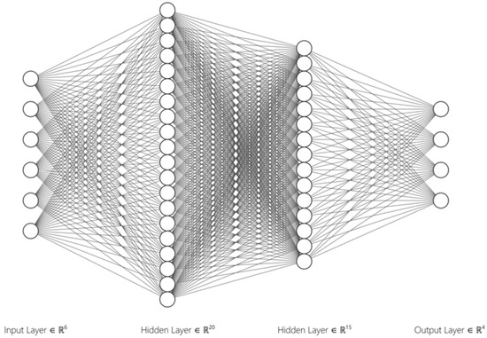
Figure 1.
Schematic representation of the artificial neural network (ANN) architecture utilized in this study. The network comprises an input layer with 6 features derived from Hilbert–Huang transform (HHT), followed by two hidden layers with 20 and 15 neurons, and an output layer with 4 neurons corresponding to the classification labels normal, sag, swell, and interruption.
The number of neurons in the hidden layers was determined empirically via multiple trials to maximize classification accuracy. However, no formal optimization method (e.g., grid search, Bayesian tuning, or genetic algorithms) was applied.
Each hidden layer employed the Rectified Linear Unit (ReLU) activation function to enhance nonlinearity and improve convergence speed, while the output layer used the Softmax function for multi-class classification.
The selection of this network structure was based on iterative experimentation. Several configurations were evaluated, including architectures with fewer neurons (e.g., 10–5) and those with additional hidden layers. Networks with fewer parameters exhibited underfitting and reduced generalization, while larger or deeper models increased training time without substantial improvements in accuracy. The 20–15 topology was selected as it offered a favorable trade-off between classification performance and computational efficiency.
No formal hyperparameter tuning methods (e.g., grid search or Bayesian optimization) were applied in this study as they were not part of this research objectives.
The network was implemented and trained in MATLAB using the Levenberg–Marquardt backpropagation algorithm and a cross-entropy loss function. Training data were generated through voltage simulations in the IEEE 33-bus system under various disturbance types and durations (0.2 s, 0.4 s, and 0.8 s). The dataset was partitioned into 70% for training, 15% for validation, and 15% for testing.
The proposed ANN configuration achieved a classification accuracy of 94.09% on the testing set, demonstrating strong generalization across different disturbance types and bus locations. Each input to the classifier corresponds to a 0.8 s window of voltage data, sampled at 10 kHz, resulting in 800 samples per event. Although the current implementation operates in offline mode, the compact feature set and lightweight network architecture are well suited for future integration into real-time disturbance monitoring systems.
2.4. Hilbert–Huang Transform
The Hilbert–Huang transform (HHT) is a time-frequency analysis method tailored for non-stationary and nonlinear signals. Unlike traditional techniques such as the Fourier or wavelet transforms that rely on predefined basis functions, the HHT is data-driven and adaptive [42,43]. It consists of two main stages:
- Empirical mode decomposition (EMD);
- Hilbert spectral analysis (HSA) via the Hilbert transform.
2.4.1. Empirical Mode Decomposition (EMD)
EMD decomposes a complex signal into a finite set of intrinsic mode functions (IMFs). Each IMF represents a simple oscillatory mode inherent to the original signal. For a function to qualify as an IMF, it must satisfy the following:
- The number of extrema and the number of zero crossings must either be equal or differ at most by one.
- The mean of the upper and lower envelopes—defined by local maxima and minima—must be zero at all points.
The step-by-step EMD process for a signal is as follows:
- Identify local maxima and minima. Construct the upper envelope and lower envelope using interpolation.
- Compute the mean:
- Subtract the mean from the signal (sifting process):
- When IMF conditions are met, set:
- Subtract from to compute the residue:
- Continue the decomposition until the final residue is obtained:
This adaptive decomposition preserves both time and frequency localization [44,45,46].
2.4.2. Hilbert Spectral Analysis (Hilbert Transform)
After extracting the IMFs via EMD, the Hilbert transform is applied to each IMF to extract instantaneous frequency and amplitude information [47,48,49].
Given a real-valued signal , its analytic representation is defined as:
where is the Hilbert transform of :
and denotes the Cauchy principal value.
From the analytic signal , the following quantities are derived:
- Instantaneous amplitude:
- Instantaneous phase:
- Instantaneous frequency:
These quantities provide a high-resolution time–frequency representation of the original signal, enabling the identification of time-localized spectral features.
2.4.3. Feature Selection and Implementation Details
For each voltage signal, EMD typically yields between six and eight intrinsic mode functions (IMFs), depending on the duration and shape of the disturbance. However, only the first two IMFs are retained for feature extraction. These contain the most relevant high-frequency content associated with transient anomalies. Higher-order IMFs, which reflect slower oscillations and baseline drift, were excluded to reduce redundancy and dimensionality.
The sifting process follows the standard algorithm with a stopping criterion based on the standard deviation between successive iterations, with a threshold of 0.2. This ensures convergence while avoiding excessive iterations. No additional denoising methods were applied, as EMD inherently acts as a signal-adaptive filter by isolating oscillatory modes.
After obtaining the relevant IMFs, the Hilbert transform is applied to each to compute the instantaneous amplitude and frequency as defined in Equations (8) and (10). From these, the following statistical features are extracted:
- Mean of the instantaneous amplitude;
- Standard deviation of the instantaneous amplitude;
- Mean of the instantaneous frequency.
These features were selected due to their ability to characterize the magnitude and frequency behavior of transient disturbances in a compact form. Preliminary testing with additional features (e.g., entropy, energy, and higher-order moments) showed marginal gains in classification accuracy while increasing the risk of overfitting and computational complexity. Therefore, the chosen features offer a robust and efficient representation for training the neural network classifiers.
2.5. Study Cases
Electrical disturbances can result from environmental factors, external events, or internal operational failures. These disruptions manifest mainly through voltage variations, such as sags, surges, or complete interruptions, which compromise system stability, accelerate equipment wear, and reduce power quality.
2.5.1. System Overview
The electrical network analyzed corresponds to the IEEE 33-bus radial distribution system. Due to its realistic configuration and widespread use, this testbed is a reference model for evaluating advanced monitoring, control, and diagnostic methodologies.
Its key features include the following:
- 33 buses and 32 distribution lines.
- Nominal voltage of 12.66 kV.
- Inclusion of various types of loads and line impedances.
- A radial structure prone to disturbances such as sags and interruptions.
Table 2 summarizes the voltage range and power values across the buses.
Table 2.
Voltage and load summary in the IEEE 33-bus system.
2.5.2. Line Impedance Profile
The impedance values across lines introduce variation in voltage drops, directly affecting disturbance propagation. Rather than listing all 33 line parameters, Table 3 presents statistical metrics to capture impedance characteristics.
Table 3.
Summary of line impedance values in the IEEE 33-bus system.
2.5.3. Simulation and Disturbance Modeling
This system was simulated using MATLAB/Simulink to test its response to voltage disturbances under controlled conditions.
The IEEE 33-bus test system is widely adopted for its radial structure, realistic voltage drops, and load diversity, making it a suitable benchmark for evaluating power quality event detection methods. It includes buses with varied electrical distances from the substation, enabling robust analysis of spatially distributed voltage anomalies.
To evaluate the classifier’s generalization across network conditions, voltage disturbances were injected at four representative buses: 4, 12, 18, and 30. These were selected to reflect a range of topological characteristics:
- Bus 4 is located near the source, experiencing minimal voltage drop.
- Bus 12 lies in the middle of the feeder.
- Bus 18 and Bus 30 are at the feeder end, where voltage sag and transient sensitivity are more severe.
Each bus underwent three disturbance durations (0.2 s, 0.4 s, 0.8 s) across all event types. This setup produced a diverse labeled dataset to train and validate the ANN classifier. Labels used for classification were previously listed in Table 1.
The IEEE 33-bus system provides a reliable environment for studying the behavior of distribution networks under anomalous operating conditions. Its structure supports the development and validation of detection algorithms and facilitates dynamic analysis of power quality events. The system’s topology is detailed in Figure 2, in which Bus 0 is referred to as the connection point to the grid.
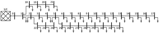
Figure 2.
IEEE 33-bus radial distribution system used for simulating power quality disturbance events, consisting of 33 buses and 32 branches arranged in a single-feeder layout. Bus 0 represents the substation or source bus, while representative disturbance cases were injected at buses 4, 12, 18, and 30 to simulate voltage anomalies at various network depths.
2.6. Methodology Algorithm
The following Algorithm 1 outlines the proposed methodology for classifying electrical disturbances in distribution systems using a hybrid approach that combines the Hilbert–Huang transform (HHT) with artificial neural networks (ANNs). The procedure begins with the controlled injection of sag, swell, and interruption events into an IEEE 33-bus test system. This is followed by decomposing the resulting voltage signals into intrinsic mode functions (IMFs) through empirical mode decomposition (EMD). Subsequently, the Hilbert transform is applied to each IMF to extract time–frequency features such as instantaneous amplitude and frequency.
| Algorithm 1 Disturbance classification method using HHT and ANN |
|
These features are used to construct descriptive input vectors for training a supervised ANN model, which accurately identifies the type of disturbance present in each scenario. The algorithm includes all stages from simulation and preprocessing to model training and validation, providing a robust framework for detecting and classifying power quality events under dynamic operating conditions.
3. Results
3.1. Case Study: Voltage Sag
The IEEE 33-bus radial distribution system is used as the simulation platform to evaluate the proposed methodology’s performance. Disturbances are introduced in the MATLAB/Simulink environment by injecting voltage sags into selected nodes using block-level modifications to the transmission lines. Figure 3 shows a visual representation of voltage sags. Three distinct sag durations are defined, 0.2 s, 0.4 s, and 0.8 s, allowing for a multi-scale analysis of the neural network’s ability to detect, classify, and localize transient events.
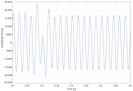
Figure 3.
Voltage signal with an artificially injected sag event starting at approximately 0.3 s and lasting 0.2 s. The signal drop reflects a simulated voltage sag used for training and evaluation of the classification model.
Results Validation
As defined in Table 1, each disturbance is assigned a numerical label to facilitate classification. Voltage sags are represented by label 3. The detection system was evaluated across multiple scenarios by introducing voltage drops at different time points. Figure 4 illustrates the network’s response to a disturbance with a s duration. The model successfully identifies the event onset and assigns the correct label with high temporal precision.
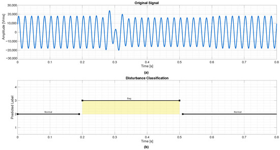
Figure 4.
Detection of a voltage sag with 0.2 s duration. (a) Original voltage signal showing a sudden drop in amplitude between 0.3 s and 0.5 s. (b) Corresponding classification output, where class labels are interruption, normal, sag, and swell.
Figure 5 shows the response to a sag with a 0.4 s duration. The classification remains consistent, with the model correctly identifying the transition between normal (label 2) and disturbed (label 3) states, and returning to label 2 once the sag ends.
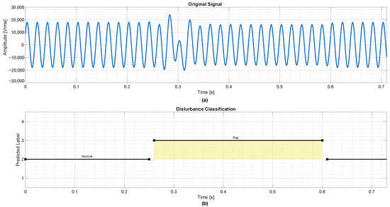
Figure 5.
Detection of a voltage sag with 0.4 s duration. (a) Original voltage signal showing a sudden drop in amplitude between 0.3 s and 0.6 s. (b) Corresponding classification output, where class labels are interruption, normal, sag, and swell.
The final test, presented in Figure 6, evaluates the detection of a longer-duration sag with 0.8 s duration. The classifier maintains its performance, demonstrating robustness in identifying the anomaly across varying time windows.
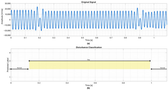
Figure 6.
Detection of a voltage sag with 0.8 s duration. (a) Original voltage signal showing a prolonged drop in amplitude from approximately 0.2 s to 1.0 s. (b) Corresponding classification output, where class labels are interruption, normal, sag, and swell.
These results confirm the classifier’s ability to accurately detect the onset, duration, and clearance of voltage sag events. The ANN demonstrates strong generalization to different temporal scales, a critical real-time power quality monitoring capability. Unlike traditional detection methods that often rely on fixed thresholds or frequency-domain analysis, the data-driven approach employed here adapts to dynamic signal behavior, offering improved flexibility and precision.
Moreover, the model’s accurate identification of the transition boundaries between normal and abnormal states supports its application in intelligent fault detection systems, where rapid response and reliable classification are essential for maintaining grid reliability and service continuity.
3.2. Case Study: Voltage Level Interruption
The IEEE 33-bus distribution system assesses the proposed methodology’s ability to detect voltage interruption events. These are modeled in MATLAB/Simulink by inserting block-level modifications that simulate a complete voltage loss at selected nodes. Three distinct durations are defined for the analysis: 0.2 s, 0.4 s, and 0.8 s. Figure 7 presents the signal behavior during one such simulated interruption. The primary objective is to validate the neural network’s capacity to identify and classify these events under varying temporal conditions.
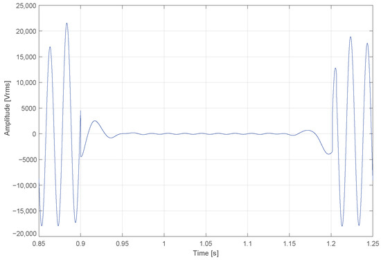
Figure 7.
Voltage signal with a simulated interruption event, showing a complete drop in amplitude from approximately 0.9 s to 1.2 s. This scenario is used to validate the model’s ability to identify sudden voltage losses under variable temporal conditions.
Results Validation
As Table 1 indicates, voltage interruptions are represented by label 1. The neural network is evaluated across three scenarios in which the interruption begins at s, s, and s, respectively. These events simulate the sudden loss of voltage due to faults, protection device operation, or equipment malfunction, all of which may lead to severe system consequences if undetected.
Figure 8 illustrates the detection output for the first case. The ANN correctly identifies the interruption onset, maintains label 1 during the disturbance window, and returns to label 2 upon signal recovery.
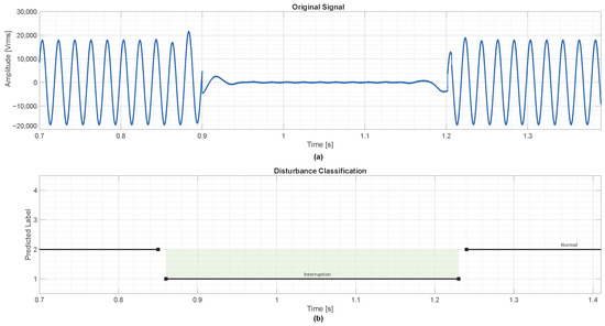
Figure 8.
Detection of a voltage interruption with 0.2 s duration. (a) Original voltage signal showing a temporary loss of amplitude between 0.9 s and 1.2 s. (b) Corresponding classification output, where class labels are interruption, normal, sag, and swell.
Figure 9 displays the detection behavior for a 0.4 s interruption. The network’s consistent response, despite variation in timing, demonstrates its generalization capability.
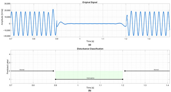
Figure 9.
Detection of a voltage interruption with 0.4 s duration. (a) Original voltage signal showing a drop to near-zero amplitude from approximately 0.9 s to 1.3 s. (b) Corresponding classification output, where class labels are interruption, normal, sag, and swell.
In the final case, shown in Figure 10, the ANN again exhibits accurate temporal labeling of the event with no misclassifications, even for the longest duration scenario.
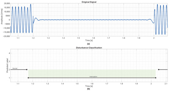
Figure 10.
Detection of a voltage interruption with 0.8 s duration. (a) Original voltage signal showing a complete amplitude drop from approximately 1.2 s to 2.0 s. (b) Corresponding classification output, where class labels are interruption, normal, sag, and swell.
The model’s consistent performance across these scenarios validates its robustness in detecting interruptions under varying durations and onset conditions. Such capabilities are essential for real-world deployment, where faults may occur unpredictably in time and magnitude.
Accurate classification of interruption events not only enables timely fault isolation but also supports the implementation of automated mitigation strategies. Therefore, the proposed supervised learning architecture strengthens early detection systems and enhances the intelligence and adaptability of modern distribution networks.
3.3. Case Study: Voltage Swell
The IEEE 33-bus distribution system is employed as the simulation framework to evaluate the model’s ability to detect swell events. In this case study, swell disturbances are introduced at selected nodes in the MATLAB/Simulink environment. These surges represent temporary increases in RMS voltage levels. Three durations are considered: 0.2 s, 0.4 s, and 0.8 s. Figure 11 illustrates the signal profile during a simulated swell event.
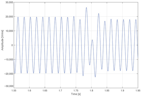
Figure 11.
Voltage signal with a simulated swell disturbance, showing a temporary increase in amplitude around 1.8 s. This profile is used to test the model’s capability to detect and classify Swell events with short durations in distribution systems.
Results Validation
According to the classification scheme in Table 1, swell events are labeled with identifier 4. The network was evaluated across three time-based scenarios, each representing a different moment of surge onset: 0.2 s, 0.4 s, and 0.8 s. These events are critical in power quality analysis, as they can severely damage sensitive electronic equipment or lead to misoperation of protection devices if not adequately addressed.
Figure 12 shows the neural network’s output for the 0.2 s surge event. The system accurately detects the start and end of the disturbance and correctly assigns label 4 throughout the duration.
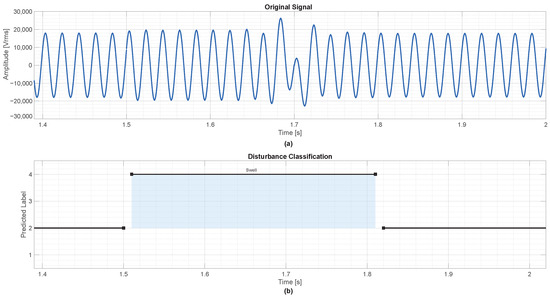
Figure 12.
Detection of an overvoltage event with 0.2 s duration. (a) Original voltage signal showing an amplitude increase between approximately 1.5 s and 1.8 s. (b) Corresponding classification output, where class labels are interruption, normal, sag, and swell.
Figure 13 presents the network’s classification for the 0.4 s case. The system demonstrates consistency by accurately labeling the anomaly and transitioning back to label 2 after the event concludes.
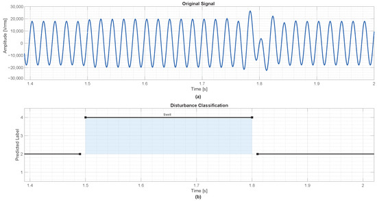
Figure 13.
Detection of an overvoltage event with 0.4 s duration. (a) Original voltage signal showing a temporary rise in amplitude between approximately 1.5 s and 1.9 s. (b) Corresponding classification output, where class labels are interruption, normal, sag, and swell.
The last test, shown in Figure 14, evaluates the most extended event duration (0.8 s). Again, the model performs reliably, marking a clear boundary between normal and disturbed states with no false positives or missed detections.
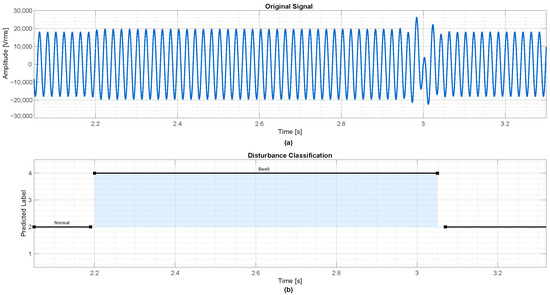
Figure 14.
Detection of an overvoltage event with 0.8 s duration. (a) Original voltage signal showing a significant amplitude increase from approximately 2.2 s to 3.0 s. (b) Corresponding classification output, where class labels are interruption, normal, sag, and swell.
The experimental results confirm the robustness of the proposed ANN-based classifier in recognizing Swell events of varying durations. The system’s ability to maintain accuracy under multiple disturbance windows supports its deployment in predictive monitoring and adaptive protection schemes. Moreover, its strong generalization across different time scales reinforces its value as a dynamic fault detection tool within innovative grid environments.
3.4. Results Summary
The Hilbert–Huang transform (HHT) was applied to extract relevant features from voltage disturbance signals in the IEEE 33-bus system. This adaptive time–frequency analysis combines empirical mode decomposition (EMD) with the Hilbert transform, enabling non-stationary signals to be decomposed into a set of intrinsic mode functions (IMFs), each capturing oscillatory behavior at different time scales. This decomposition facilitates the separation of fundamental signal components from transient irregularities, allowing for high-resolution and localized characterization of electrical disturbances.
Applying the Hilbert transform to each IMF yields instantaneous amplitude, phase, and frequency parameters. These descriptors form a detailed representation of the signal’s dynamic evolution, particularly beneficial for identifying the timing, duration, and severity of non-stationary disturbances. Figure 15 illustrates this process for the first IMF, where high-resolution time–frequency data enables precise anomaly detection.
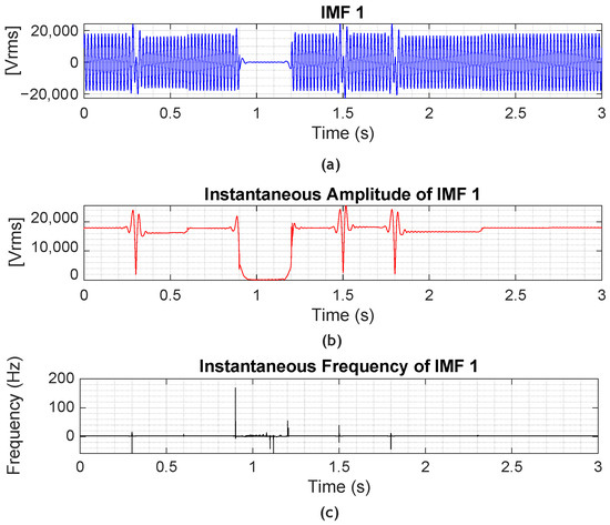
Figure 15.
Hilbert–Huang analysis results for IMF 1. (a) Extracted IMF 1 component from the original voltage signal. (b) Instantaneous amplitude profile of IMF 1, highlighting energy variations during disturbances. (c) Instantaneous frequency extracted via the Hilbert transform, capturing spectral shifts across time.
As shown in Figure 16, the visualization of each IMF’s amplitude and frequency spectrum allows for identifying both abrupt and subtle alterations in the signal. This capability makes the HHT framework a powerful tool for advanced power quality assessment and transient event localization in modern distribution networks.
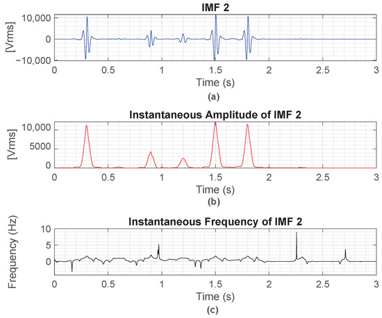
Figure 16.
Hilbert–Huang analysis results for IMF 2. (a) Extracted IMF 2 component, representing lower-frequency oscillations. (b) Instantaneous amplitude of IMF 2, highlighting transient energy bursts. (c) Instantaneous frequency content captures subtle dynamic variations associated with event transitions.
Once the HHT-transformed signals were used as training inputs, the neural network was optimized using a performance-based validation approach. As shown in Figure 17, the model achieved a classification error of 0.125 across 250,000 data samples. The rapid convergence observed demonstrates successful generalization and training stability.
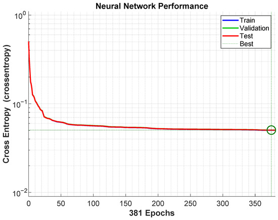
Figure 17.
Training performance of the neural network over 381 epochs using the cross-entropy loss function. The curves represent the evolution of training, validation, and testing errors, with the green circle marking the best validation performance. The convergence trend indicates stable learning and minimal overfitting.
To evaluate the generalization of the model under complex operating conditions, additional case studies were developed using a realistic simulation of the IEEE 33-bus system. In each scenario, simultaneous disturbances (sags, interruptions, and swells) were injected across all three phases at multiple time points ( s, s, and s). In Case 1 (Figure 18), the model successfully identified the type, timing, and duration of each event, demonstrating its ability to differentiate among label classes with no misclassification.
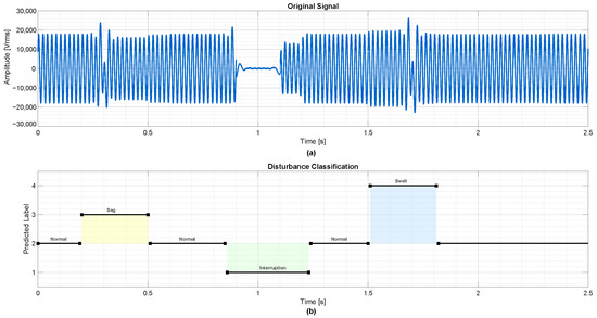
Figure 18.
Case 1: Neural network classification of a composite disturbance scenario with events occurring at s (sag), s (interruption), and s (swell). (a) Original voltage signal showing distinct amplitude variations for each disturbance type. (b) Corresponding classification output, accurately identifying and labeling each event in time. Class labels: interruption, normal, sag, swell.
Figure 19 shows the system’s response to the second event set. The classifier maintained high precision in distinguishing transitions between normal (label 2), interruptions (label 1), sags (label 3), and swells (label 4). This highlights the model’s robustness against temporal variability in fault occurrence.
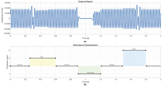
Figure 19.
Case 2: Neural network classification of a composite disturbance scenario with events occurring at s (sag), s (interruption), and s (swell). (a) Original voltage signal illustrating distinct drops and surges in amplitude. (b) Predicted class labels accurately track each disturbance type and transition, confirming the classifier’s temporal sensitivity and robustness. Class labels: interruption, normal, sag, swell.
The third test, presented in Figure 20, validated the network’s ability to detect extended and overlapping anomalies under multiphase symmetrical conditions. The classifier’s consistent behavior across all tests confirms its high generalization capacity and resilience to complex dynamic operating states.
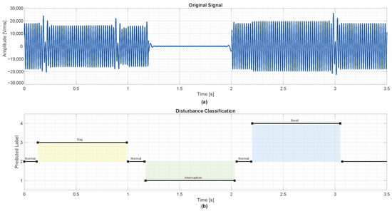
Figure 20.
Case 3: Neural network classification for a multievent sequence beginning at s. (a) Voltage signal exhibiting sequential voltage sag, interruption, and swell phenomena. (b) Predicted class labels show accurate transitions across all events, highlighting the model’s robustness in handling composite disturbances. Class labels: interruption, normal, sag, swell.
Overall, the combined use of the HHT and neural networks provides a comprehensive and adaptive strategy for real-time monitoring. The model not only detects and classifies transient disturbances with high precision but also retains performance under multiphase, time-variable conditions. This positions the approach as a scalable and intelligent solution for power quality assurance and advanced fault diagnostics in modern distribution grids.
The results obtained demonstrate the effectiveness of the proposed HHT-based ANN classification framework in fulfilling the primary objectives of this study. The model achieved an overall classification accuracy of 94.09%, with strong generalization across varying disturbance durations (0.2 s, 0.4 s, 0.8 s) and spatial locations within the IEEE 33-bus system. The confusion matrix shows that the classifier reliably distinguishes between voltage sag, swell, and interruption events, each associated with distinct voltage signatures defined by IEEE 1159.
The relatively shallow ANN architecture enabled fast convergence (as seen in the training curve) while maintaining low computational complexity, making the approach suitable for real-time deployment. These results confirm that the integration of HHT features (instantaneous amplitude and frequency) provides a rich, non-stationary feature space that enhances the classifier’s ability to detect subtle transient patterns.
Furthermore, the method’s robustness across buses and time windows suggests that it can be effectively deployed in smart distribution networks where operating conditions are dynamic and disturbance propagation is topology-dependent. Thus, the presented results validate the proposed approach not only in terms of raw performance metrics but also in terms of its alignment with real-world monitoring requirements.
3.5. Expanded Experimental Validation
The training dataset was constructed using simulated voltage signals in the IEEE 33-bus test system under four event classes: normal operation and voltage sag, swell, and interruption. Each class contains 300 labeled signals per duration (0.2 s, 0.4 s, and 0.8 s), yielding a total of 3600 signals. Disturbance events were injected with randomized onset times, amplitudes, and durations within the IEEE 1159-2019 guidelines. Voltage sags varied between 60 and 90% of nominal voltage, swells between 110 and 130%, and interruptions dropped below 10% for specified intervals. No synthetic noise was added, but signal diversity was ensured through perturbation variability and randomized bus locations.
To assess generalization capability, we adopted five-fold cross-validation over a stratified 80/20 training/test split, ensuring that all event types and durations were proportionally represented across folds. This method provides robust performance estimation and reduces the risk of overfitting, comparable to using an independent test set, without requiring additional simulations. The average classification accuracy across folds was 94.09%, with standard deviation below 1%, confirming stable model behavior.
A confusion matrix summarizing classification outcomes is shown in Figure 21, with strong per-class separability. Table 4 provides precision, recall, and F1-score metrics for each class, highlighting the model’s balanced accuracy across all types of disturbances.
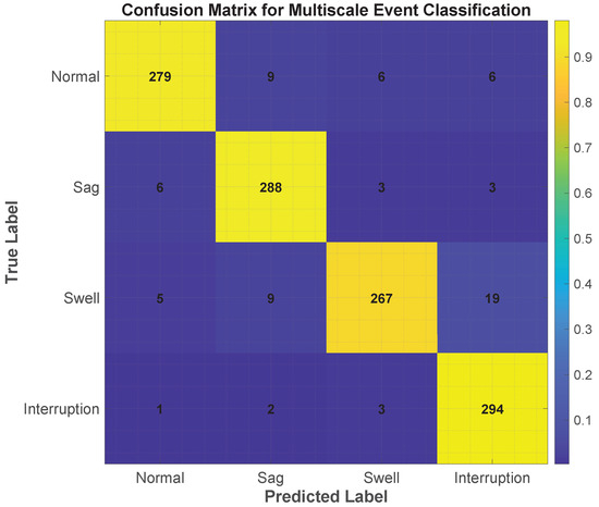
Figure 21.
Confusion matrix illustrating the classification performance of the proposed ANN model across four event types: normal, sag, swell, and interruption. Diagonal values indicate correct classifications, while off-diagonal values represent misclassifications. Color intensity reflects the normalized frequency of predictions. The model demonstrates strong accuracy, particularly for interruption and normal events.
Table 4.
Per-class performance metrics.
To formally define these metrics:
- Precision:
- Recall:
- F1-score:
Although a comparison with other classifiers (e.g., SVM, decision tree) could offer additional insight, the focus of this work was to validate the neural network approach under multiscale event durations using a consistent, diverse dataset. Given the satisfactory results and robust generalization observed through cross-validation, extending the study to alternative classifiers is considered future work.
Real-Time Feasibility and Computational Cost
Although real-time deployment was not directly implemented, the methodology was designed with computational efficiency in mind. The average processing time per event, including both Hilbert–Huang decomposition and ANN classification, was approximately 0.13 s using MATLAB on a standard Intel i7-11800H CPU with 16 GB RAM. This runtime supports near real-time monitoring scenarios (e.g., 5 Hz sampling) with minimal optimization.
This result aligns with reported empirical runtimes for Hilbert–Huang transform (HHT)-based feature extraction in non-parallelized settings, where typical values range between 0.1 and 0.2 s per signal for similar data lengths [50,51]. Furthermore, the proposed ANN architecture remains lightweight, with fewer than 100 trainable parameters, enabling fast inference and compatibility with embedded or edge-device platforms in smart grid environments.
Comparative Analysis with Existing Methods
To evaluate the results from the implementation of the HHT-derived ANN model, in Table 5, this paper reviews other approaches to power quality disturbance (PQD) classification, focusing on more recent published works, which naturally enables understanding where the gaps in the research lie. The table features the most impactful works published after 2020 that use other signal processing and machine learning techniques like Discrete Wavelet Transform (DWT), Variational Mode Decomposition (VMD), and S-Transform, alongside Support Vector Machine (SVM), Convolutional Neural Network (CNN), and Extreme Learning Machine (ELM) classifiers.
Table 5.
Comparison of recent PQD classification methodologies (2020–2025).
While some methods like DWT combined with FPGA-accelerated ELMs reach classification accuracies over 99%, these methods often rely on ideal signal conditions or need specialized equipment. In comparison, the approach presented in this paper attained 94.09% classification accuracy while processing each event in 0.13 s on a standard CPU. This trade-off between accuracy and efficiency highlights the method’s potential for real-time application in smart distribution systems. In addition, the application of Hilbert–Huang transform allows for multiscale analysis of changing voltage signals and provides a powerful complement to standard time–frequency decomposition methods.
4. Conclusions
The neural network model trained using features obtained with the Hilbert–Huang transform reached a classification accuracy of 94.09% for electrical system disturbance classification. The level of accuracy attained confirms the model is well-suited for the automatic detection of transient events, underscoring its value for proactive power quality monitoring.
The architectural model described herein displayed a high level of generalization, performing voltage dip detection and interruption detection, as well as recording overrides of the voltage at 0.2, 0.4, and 0.8 s. In all scenarios studied, the neural network was successful in detecting the beginning, active period, and termination of the event without any false detections.
As the ANN relies on features derived from the Hilbert–Huang transform—namely, the instantaneous amplitude and frequency extracted from the first two IMFs—the HHT remains an integral part of the inference pipeline. However, due to the localized and adaptive nature of the EMD–Hilbert process, feature extraction can be performed efficiently, supporting the feasibility of deploying the proposed method in real-time disturbance monitoring systems.
While simulating simultaneous active disturbances on all three phases of the 33 node IEEE system, the model consistently demonstrated accurate classification devoid of errors. The ability to sustain this level of performance illustrates the capacity of the system to function in highly dynamic scenarios, which is necessary in modern distribution systems that are subject to high-load fluctuations and transients.
The current framework was evaluated using synthetic, noise-free voltage signals under controlled scenarios. Although the results demonstrate strong classification accuracy, practical deployment may face challenges such as measurement noise, data incompleteness, or signal distortions. Future research will aim to validate the model on field-acquired datasets and explore alternative neural architectures, such as convolutional or recurrent networks, to enhance generalization under real-world conditions.
5. Future Work and Challenges
Based on the results obtained, one of the central future projections is to apply the proposed model to the analysis of short-circuit conditions in distribution networks. This type of event represents one of the most critical scenarios in the operation of electrical systems, and its early detection is key to avoiding severe damage to the infrastructure. Incorporating short circuits as a new disturbance class within the classification system would enable the evaluation of the model’s ability to identify high-severity events, accurately differentiating them from other, less severe, transient phenomena.
Another relevant aspect of future work will be the validation of the model with real signals obtained directly from operating electrical networks. This approach will allow for the analysis of its behavior under practical conditions characterized by noise, uncertainty, and multiple sources of interference. Additionally, the exploration of more sophisticated neural architectures, such as convolutional networks (CNNs), recurrent networks (RNNs), or hybrid networks, is proposed, which could improve accuracy, reduce response times, and increase the system’s robustness to non-ideal or incomplete data.
Additionally, while this study focused on the voltage response at the point of disturbance injection, it is important to note that power quality events often propagate to adjacent buses, especially in radial networks. These neighboring locations may experience more severe or earlier voltage deviations due to impedance paths and electrical proximity. As such, future work will explore spatial feature integration by capturing the voltage behavior of adjacent buses to enhance detection accuracy and resilience. This approach will support distributed sensing schemes and better reflect real-world deployment scenarios in active distribution networks.
The proposed methodology was designed with implementation feasibility in mind. By leveraging a lightweight neural architecture and using HHT-derived statistical features, the framework avoids the high computational overhead typical of more complex models such as deep CNNs or ensemble classifiers. This makes it suitable for deployment on embedded platforms or edge devices for real-time monitoring applications.
While the current validation is based on simulation, the approach is modular and can be adapted to process real-time voltage signals from existing smart meters or phasor measurement units (PMUs). While the classifier achieved high accuracy (94.09%) and consistent recall across all event types, future studies could explore real-time adaptation and alternative network architectures to enhance robustness and reduce latency in practical deployment scenarios. Integration efforts will also focus on hardware-in-the-loop validation and compatibility with modern grid monitoring infrastructure, paving the way for scalable, accurate, and responsive power quality monitoring in active distribution networks.
Finally, we propose integrating the model into real-time monitoring platforms, such as SCADA systems or embedded environments (such as Raspberry Pi or FPGA), to enable continuous monitoring of electrical service quality. This implementation would not only enable efficient disturbance detection but also facilitate the development of automatic response schemes that respond promptly to anomalous events. Together, these future directions position the proposed approach as a solid foundation for designing intelligent protection and diagnostic systems in modern distribution networks.
Author Contributions
J.V.: conceptualization, methodology, validation, writing—review and editing, data curation, formal analysis. M.J.: conceptualization, methodology, validation, writing—review and editing, data curation, formal analysis. D.C.: methodology, validation, writing—review and editing. All authors have read and agreed to the published version of the manuscript.
Funding
Universidad Politécnica Salesiana and GIREI supported this work—Smart Grid Research Group under the project “Optimization of Energy Dispatch in Block H of the Salesian Polytechnic University, Quito South Campus, through a Predictive Consumption Model and Hybrid Management between Solar Panels and the Electric Grid” approved and founded by resolution 005-01-2025-02-07.
Institutional Review Board Statement
Not applicable.
Informed Consent Statement
Not applicable.
Data Availability Statement
The original contributions presented in the study are included in the article, further inquiries can be directed to the corresponding author.
Conflicts of Interest
The authors declare no conflicts of interest.
Abbreviations
The following abbreviations are used in this manuscript:
| Hilbert–Huang transform | |
| Empirical mode decomposition | |
| Intrinsic mode function | |
| Artificial neural network | |
| Instantaneous amplitude of the signal | |
| Instantaneous phase of the signal | |
| Instantaneous frequency of the signal | |
| Original voltage signal in time domain | |
| Analytic signal derived from | |
| Hilbert transform of | |
| k-th intrinsic mode function | |
| Residual signal after extracting k IMFs | |
| Mean envelope used in EMD | |
| Instantaneous amplitude of IMF k | |
| Instantaneous frequency of IMF k | |
| Instantaneous phase of IMF k | |
| t | Time (in seconds) |
| IEEE 33-bus test system | |
| Disturbance duration in seconds | |
| Signal at node i under disturbance d | |
| Feature vector for signal i | |
| Class label for signal i | |
| Predicted output of the ANN | |
| Weights of the trained neural network | |
| Loss function comparing ground truth and prediction | |
| True positive | |
| False positive | |
| False negative | |
| Label 1 | Interruption |
| Label 2 | Normal |
| Label 3 | Voltage sag |
| Label 4 | Voltage swell |
References
- Tiwari, D.; Zideh, M.J.; Talreja, V.; Verma, V.; Solanki, S.K.; Solanki, J. Power Flow Analysis Using Deep Neural Networks in Three-Phase Unbalanced Smart Distribution Grids. In Proceedings of the 2024 IEEE Power & Energy Society General Meeting (PESGM), Seattle, WA, USA, 21–25 July 2024; pp. 1–5. [Google Scholar] [CrossRef]
- Sharma, S. Coordination of Transmission and Distribution Systems in Load Restoration. In Proceedings of the 2024 IEEE Power & Energy Society Innovative Smart Grid Technologies Conference (ISGT), Bengaluru, India, 10–13 November 2024; pp. 300–305. [Google Scholar] [CrossRef]
- Technical Report Std 1159-2019; IEEE Recommended Practice for Monitoring Electric Power Quality. IEEE Power and Energy Society: New York, NY, USA, 2019. [CrossRef]
- Chidurala, A.; Saha, T.K.; Mithulananthan, N. Harmonic Emissions Assessment of Distributed Photovoltaic Systems in Low Voltage Network. In Proceedings of the 2023 Middle East and North Africa Solar Conference (MENA-SC), Dubai, United Arab Emirates, 15–18 November 2023; pp. 1443–1452. [Google Scholar] [CrossRef]
- Zhang, Y.; Li, Y.; Wang, X. Application of Artificial Intelligence Technology in Power Equipment Condition Prediction and Maintenance. In Proceedings of the 2023 International Conference on Artificial Intelligence, Kobe, Japan, 20–22 March 2023. [Google Scholar] [CrossRef]
- Rayudu, D.V.; Roseline, J.F. Accurate Weather Forecasting for Rainfall Prediction Using Artificial Neural Network Compared with Deep Learning Neural Network. In Proceedings of the 2023 International Conference on Artificial Intelligence and Knowledge Discovery in Concurrent Engineering (ICECONF), Chennai, India, 5–7 January 2023; pp. 1–6. [Google Scholar] [CrossRef]
- Ompokov, V.D.; Boronoev, V.V. Mode Decomposition and the Hilbert-Huang Transform. In Proceedings of the 2019 Russian Open Conference on Radio Wave Propagation (RWP), Kazan, Russia, 1–6 July 2019. [Google Scholar] [CrossRef]
- Alshumayri, K.A.; Shafiullah, M. Distribution Grid Fault Diagnostic Employing Hilbert-Huang Transform and Neural Networks. In Proceedings of the 2022 International Conference on Power Energy Systems and Applications (ICoPESA), Singapore, 25–27 February 2022; pp. 263–268. [Google Scholar] [CrossRef]
- Rosero-Morillo, V.A.; Gonzalez-Longatt, F.; Quispe, J.C.; Salazar, E.J.; Orduña, E.; Samper, M.E. Emerging Trends in Active Distribution Network Fault Detection. Renew. Energy Focus 2025, 53, 100684. [Google Scholar] [CrossRef]
- Haydaroğlu, C.; Kılıç, H.; Gümüş, B.; Özdemir, M.T. Advancing Fault Detection in Distribution Networks with a Real-Time Approach Using Robust RVFLN. Appl. Sci. 2025, 15, 1908. [Google Scholar] [CrossRef]
- Adewole, A.C.; Rajapakse, A.D.; Ouellette, D.; Forsyth, P. Protection of active distribution networks incorporating microgrids with multi-technology distributed energy resources. Electr. Power Syst. Res. 2022, 202, 107575. [Google Scholar] [CrossRef]
- Aziz, T.; Ketjoy, N. PV Penetration Limits in Low Voltage Networks and Voltage Variations. IEEE Access 2017, 5, 16784–16792. [Google Scholar] [CrossRef]
- Majeed, A.A.; Altaie, A.S.; Abderrahim, M.; Alkhazraji, A. A Review of Protection Schemes for Electrical Distribution Networks with Green Distributed Generation. Energies 2023, 16, 7587. [Google Scholar] [CrossRef]
- Lagos, D.; Papaspiliotopoulos, V.; Korres, G.; Hatziargyriou, N. Microgrid Protection against Internal Faults: Challenges in Islanded and Interconnected Operation. IEEE Power Energy Mag. 2021, 19, 20–35. [Google Scholar] [CrossRef]
- Nsaif, Y.M.; Lipu, M.S.H.; Ayob, A.; Yusof, Y.; Hussain, A. Fault Detection and Protection Schemes for Distributed Generation Integrated to Distribution Network: Challenges and Suggestions. IEEE Access 2021, 9, 142693–142717. [Google Scholar] [CrossRef]
- Conti, S. Analysis of distribution network protection issues in presence of dispersed generation. Electr. Power Syst. Res. 2009, 79, 49–56. [Google Scholar] [CrossRef]
- Samanta, I.S.; Mohanty, S.; Parida, S.M.; Rout, P.K.; Panda, S.; Bajaj, M.; Blazek, V.; Prokop, L.; Misak, S. Artificial intelligence and machine learning techniques for power quality event classification: A focused review and future insights. Results Eng. 2025, 25, 103873. [Google Scholar] [CrossRef]
- Dwivedi, D.; Babu, K.V.S.M.; Chakraborty, P.; Pal, M. Simplicial complexes using vector visibility graphs for multivariate classification of faults in electrical distribution systems. Comput. Electr. Eng. 2025, 123, 110114. [Google Scholar] [CrossRef]
- Yang, M.; Zhou, Q.; Huang, H.; Liu, J.; Pan, H.; Cheng, Y.; Kang, Z.; Hu, Z.; Hu, Y. A fault prediction method for CMOR bearings based on parameter-optimized variational mode decomposition and autocorrelation function. Fusion Eng. Des. 2025, 212, 114863. [Google Scholar] [CrossRef]
- Razeghi Jahromi, M.; Choobineh, M. Feature-based High Impedance Fault Detection in the Distribution System Using Hilbert and Fourier Transforms. In Proceedings of the IEEE Power Engineering Society Transmission and Distribution Conference, Anaheim, CA, USA, 6–9 May 2024. [Google Scholar] [CrossRef]
- Gong, Y.; Jiang, Y.; Cheng, C.; Chen, H.; Wang, S. A Deep Echo State Network with Scaling Factor Activation Functions for Fault Diagnosis of Electrical Drive Systems. IEEE Trans. Transp. Electrif. 2025, 11, 7874–7884. [Google Scholar] [CrossRef]
- Nayak, P.; Das, S.R.; Mallick, R.K.; Mishra, S.; Althobaiti, A.; Mohammad, A.; Aymen, F. 2D-convolutional neural network based fault detection and classification of transmission lines using scalogram images. Heliyon 2024, 10, e38947. [Google Scholar] [CrossRef] [PubMed]
- Razmi, P.; Pashaei, M.; Karimi, M.; Kauhaniemi, K.; Simoes, M.G. Data-Driven Intermittent Earth Fault Detection in Compensated and Isolated MV Networks. In Proceedings of the 2024 International Workshop on Artificial Intelligence and Machine Learning for Energy Transformation, AIE 2024, Vaasa, Finland, 20–22 May 2024. [Google Scholar] [CrossRef]
- Cao, Y.; Tang, J.; Shi, S.; Cai, D.; Zhang, L.; Xiong, P. Fault Diagnosis Techniques for Electrical Distribution Network Based on Artificial Intelligence and Signal Processing: A Review. Processes 2025, 13, 48. [Google Scholar] [CrossRef]
- Louzada, A.O.; Souza, W.A.; Vitor, A.L.O.; Castoldi, M.F.; Goedtel, A. Detection of Stator Faults in Three-Phase Induction Motors Using Stray Flux and Machine Learning. Energies 2025, 18, 1516. [Google Scholar] [CrossRef]
- Arévalo, P.; Cano, A.; Benavides, D.; Jurado, F. Fault analysis in clustered microgrids utilizing SVM-CNN and differential protection. Appl. Soft Comput. 2024, 164, 112031. [Google Scholar] [CrossRef]
- Vishal, M.; Kamal, A.; Viji, D. Electrical fault detection using machine learning algorithm. In Proceedings of the AIP Conference Proceedings, Zlín, Czech Republic, 26–27 July 2023; Volume 2782. [Google Scholar] [CrossRef]
- Anand, A.; Affijulla, S. Hilbert-Huang transform based fault identification and classification technique for AC power transmission line protection. Int. Trans. Electr. Energy Syst. 2020, 30, e12558. [Google Scholar] [CrossRef]
- El-Dalahmeh, M.; Al-Greer, M.; Bashir, I.; El-Dalahmeh, M.; Demirel, A.; Keysan, O. Autonomous fault detection and diagnosis for permanent magnet synchronous motors using combined variational mode decomposition, the Hilbert-Huang transform, and a convolutional neural network. Comput. Electr. Eng. 2023, 110, 108894. [Google Scholar] [CrossRef]
- Nsaif, Y.M.; Lipu, M.S.H.; Hussain, A.; Ayob, A.; Yusof, Y.; Zainuri, M.A.A.M. A Novel Fault Detection and Classification Strategy for Photovoltaic Distribution Network Using Improved Hilbert–Huang Transform and Ensemble Learning Technique. Sustainability 2022, 14, 11749. [Google Scholar] [CrossRef]
- Lu, Z. Review on mechano-electronic device fault diagnosis based on Hilbert-Huang Transformation. In Proceedings of the Journal of Physics: Conference Series, Shenzhen, China, 16–19 September 2022; Volume 2351. [Google Scholar] [CrossRef]
- Marcos-Andrade, D.; Beltran-Carbajal, F.; Esquivel-Cruz, E.; Rivas-Cambero, I.; Gabbar, H.A.; Castelan-Perez, A. Power Signal Analysis for Early Fault Detection in Brushless DC Motor Drivers Based on the Hilbert–Huang Transform. World Electr. Veh. J. 2024, 15, 159. [Google Scholar] [CrossRef]
- Torabi, M.; Alinejad-Beromi, Y. An effective Hilbert-Huang transform-based approach for dynamic eccentricity fault diagnosis in double-rotor double-sided stator structure axial flux permanent magnet generator under various load and speed conditions. Turk. J. Electr. Eng. Comput. Sci. 2023, 31, 53–76. [Google Scholar] [CrossRef]
- Zhao, S.; Chen, Y.; Rehman, A.U.; Liang, F.; Wang, S.; Zhao, Y.; Deng, W.; Ma, Y.; Cheng, Y. The Inter-turns Short Circuit Fault Detection based on External Leakage Flux Sensing and VMD-HHT Analytical Method for DFIG. In Proceedings of the ICSMD 2021—2nd International Conference on Sensing, Measurement and Data Analytics in the Era of Artificial Intelligence, Nanjing, China, 21–23 October 2021. [Google Scholar] [CrossRef]
- Romero-Carrión, D.P.; Carrión-Galarza, D.F. Análisis Bibliométrico de la Planeación de Expansión de los Sistemas Eléctricos de Potencia. In Proceedings of the 2021 IEEE Colombian Conference on Communications and Computing (COLCOM), Virtual, 26–28 May 2021; pp. 600–605. Available online: http://www.scielo.org.co/scielo.php?script=sci_arttext&pid=S1692-17982021000200150 (accessed on 3 June 2025).
- Majumdar, N.; Sarstedt, M.; Hofmann, L. Distribution Grid Power Flexibility Aggregation at Multiple Interconnections Between the High and Extra High Voltage Grid Levels. In Proceedings of the 2023 IEEE International Conference on Smart Grid and Clean Energy Technologies (ICSGCE), Kuala Lumpur, Malaysia, 13–15 October 2023; pp. 500–505. [Google Scholar] [CrossRef]
- Dawood, Z.; Babulal, C.K. Power Quality Disturbance Classification Based on Efficient Adaptive Arrhenius Artificial Bee Colony Feature Selection. Int. Trans. Electr. Energy Syst. 2021, 31, e12868. [Google Scholar] [CrossRef]
- Kazemi, A.; Ghassemi, H.; Ranjbar, A.M. Power Quality Assessment Using Hilbert-Huang Transform and Deep Neural Network. Electr. Power Syst. Res. 2021, 194, 107059. [Google Scholar] [CrossRef]
- Panigrahi, C.K.; Das, S. A Review on Power Quality Disturbance Detection and Classification Using Artificial Intelligence Techniques. Int. J. Electr. Power Energy Syst. 2020, 120, 105951. [Google Scholar] [CrossRef]
- Jumani, T.A.; Mustafa, M.W.; Alghamdi, A.S.; Rasid, M.M.; Alamgir, A.; Awan, A.B. Swarm Intelligence-Based Optimization Techniques for Dynamic Response and Power Quality Enhancement of AC Microgrids: A Comprehensive Review. IEEE Access 2020, 8, 75986–76001. [Google Scholar] [CrossRef]
- Mishra, S.; Bhende, C.N.; Panigrahi, B.K. Detection and Classification of Power Quality Disturbances Using S-Transform and Probabilistic Neural Network. IEEE Trans. Power Deliv. 2008, 23, 280–287. [Google Scholar] [CrossRef]
- Koley, B.; Das, S. Hilbert-Huang Transform Based Power Quality Event Detection Using Fuzzy Classifier. Int. J. Electr. Power & Energy Syst. 2016, 77, 346–356. [Google Scholar] [CrossRef]
- Chithra, R.; Rajaram, M. Recognition and Classification of Power Quality Disturbances Using Wavelet Based Artificial Neural Network. Int. J. Electr. Power Energy Syst. 2016, 74, 10–18. [Google Scholar] [CrossRef]
- Alhamrouni, I.; Abdul Kahar, N.H.; Salem, M.; Swadi, M.; Zahroui, Y.; Kadhim, D.J.; Mohamed, F.A.; Alhuyi Nazari, M. A Comprehensive Review on the Role of Artificial Intelligence in Power System Stability, Control, and Protection: Insights and Future Directions. Appl. Sci. 2024, 14, 6214. [Google Scholar] [CrossRef]
- He, Y.; Li, J. A Novel Approach for Power Quality Disturbance Recognition Using Improved Hilbert-Huang Transform and Deep Belief Network. Neurocomputing 2015, 149, 1333–1342. [Google Scholar] [CrossRef]
- Ghosh, S.; Lubkeman, D. An Intelligent System for Power Quality Disturbance Detection Using Wavelet and Neural Networks. Electr. Power Syst. Res. 2014, 116, 50–59. [Google Scholar] [CrossRef]
- Kumar, R.; Singh, B.; Shahani, D.T.; Chandra, A.; Al-Haddad, K. Recognition of Power-Quality Disturbances Using S-Transform-Based ANN Classifier and Rule-Based Decision Tree. IEEE Trans. Ind. Appl. 2015, 51, 1249–1258. [Google Scholar] [CrossRef]
- Luo, C.; Fan, Z. Power Quality Disturbance Classification Using Hilbert-Huang Transform and Probabilistic Neural Network. Expert Syst. Appl. 2012, 39, 6556–6565. [Google Scholar] [CrossRef]
- Wang, H.; Wang, P.; Liu, T. Power Quality Disturbance Classification Using the S-Transform and Probabilistic Neural Network. Energies 2017, 10, 107. [Google Scholar] [CrossRef]
- Li, J.; Liu, H.; Wang, D.; Bi, T. Classi fi cation of Power Quality Disturbance Based on S-Transform and Convolution Neural Network. Front. Energy Res. 2021, 9, 1–11. [Google Scholar] [CrossRef]
- Wang, J.; Xu, Z.; Che, Y. Power Quality Disturbance Classification Based on DWT and Multilayer Perceptron Extreme Learning Machine. Appl. Sci. 2020, 9, 2315. [Google Scholar] [CrossRef]
- Dutt, P.V.B.P.; Balaga, H. Detection and Classification of Power Quality Disturbances Using Variational Mode Decomposition and Deep Learning Networks. In Flexible Electronics for Electric Vehicles; Goyal, S.K., Palwalia, D.K., Tiwari, R., Gupta, Y., Eds.; Springer Nature: Singapore, 2024; pp. 1–12. [Google Scholar] [CrossRef]
- Güvengir, U.; Küçük, D.; Buhan, S.; Mantaş, C.A.; Yeniceli, M. Classification of power quality events in the transmission grid: Comparative evaluation of different machine learning models. arXiv 2025, arXiv:2503.13566. [Google Scholar] [CrossRef]
- Dubey, R.K. Power Quality Event Recognition and Classification Using an Online Sequential Extreme Learning Machine Network based on Wavelets. arXiv 2022, arXiv:2212.13375. [Google Scholar] [CrossRef]
Disclaimer/Publisher’s Note: The statements, opinions and data contained in all publications are solely those of the individual author(s) and contributor(s) and not of MDPI and/or the editor(s). MDPI and/or the editor(s) disclaim responsibility for any injury to people or property resulting from any ideas, methods, instructions or products referred to in the content. |
© 2025 by the authors. Licensee MDPI, Basel, Switzerland. This article is an open access article distributed under the terms and conditions of the Creative Commons Attribution (CC BY) license (https://creativecommons.org/licenses/by/4.0/).