Article

Lightweight Periodic Scheduler in Wearable Devices for Real-Time Biofeedback Systems in Sports and Physical Rehabilitation †

1
Faculty of Electrical Engineering, University of Ljubljana, Tržaška cesta 25, 1000 Ljubljana, Slovenia
2
Faculty of Natural Sciences and Engineering, University of Ljubljana, Aškerčeva cesta 12, 1000 Ljubljana, Slovenia
*
Author to whom correspondence should be addressed.
This article is a revised and expanded version of a paper entitled Affordable Wearable Devices with Low-Latency Wireless Communication, presented at 2023 IEEE AFRICON. Kos, A.; Tomažič, S.; Umek, A. Affordable Wearable Devices with Low-Latency Wireless Communication. In Proceedings of the 2023 IEEE AFRICON, Nairobi, Kenya, 20–22 September 2023; IEEE: Piscataway, NJ, USA; pp. 1–5.
Appl. Sci. 2025, 15(12), 6405; https://doi.org/10.3390/app15126405
Submission received: 21 February 2025 / Revised: 16 May 2025 / Accepted: 28 May 2025 / Published: 6 June 2025

Abstract

This study explores the application of wireless wearable devices within the emerging domain of biomechanical feedback systems for sports and rehabilitation. A critical aspect of these systems is the need for real-time operation, where wearable devices must execute multiple processes concurrently while ensuring specific tasks are performed within precise time constraints. To address this challenge, we developed a specialized, lightweight periodic scheduler for microcontrollers. Extensive testing under various conditions demonstrated that sensor sampling frequencies of 650 Hz and 1750 Hz are achievable when utilizing one and 26 sensor samples per packet, respectively. Receiver delays were observed to be a few milliseconds or more, depending on the application scenario. These findings offer practical guidelines for developers and practitioners working with real-time biomechanical feedback systems. By optimizing sensor sampling frequencies and packet configurations, our approach enables more responsive and accurate feedback for athletes and patients, improving the reliability of motion analysis, rehabilitation monitoring, and training assessments. Additionally, we outline the limitations of such systems in terms of transmission delays and jitter, providing insights into their feasibility for different real-world applications.

1. Introduction

Advancements in Information and Communication Technology (ICT) have significantly contributed to various research fields, thereby enhancing overall quality of life. Engaging in sufficient physical activity—whether through recreational pursuits, amateur involvement, or professional sports—is vital for maintaining health and well-being. A diverse array of devices and systems, varying in complexity, are employed to record and evaluate physical activity by measuring parameters such as daily step counts and analyze movements during athletic activities.
The integration of ICT is particularly impactful in the development of biomechanical feedback systems for sports and rehabilitation, which we address in this paper. These systems aim to acquire, monitor, analyze, assess, and improve human movement patterns in real time. While initially developed for sports performance enhancement, biomechanical feedback has also found applications in physical rehabilitation, helping patients regain mobility and correct movement patterns [1,2].
Biomechanical feedback systems are implemented with different types of devices, from professional high-precision motion capture systems to commercial mass products such as wristbands. While the former provide detailed data on the activity or movement of a specific body part, they are also expensive and require trained professionals and an adapted environment for use. The latter, on the other hand, are primarily intended for recreational use and generally only provide simple statistical data on activity. In light of the above, it is clear that we need devices that fill the gap between the two extremes. These are usually devices that are designed for a specific sport, activity, or even just a single movement. Most of these devices are wearable devices that do not interfere with activity and have wireless connectivity. These devices are worn on the body as accessories, attachments, or implants and encompass a broad spectrum—from smart devices like smartphones and smartwatches to small accessories such as smart eyewear, and specialized sensor devices or intelligent sports equipment [3]. The commercially available devices mentioned are only intended for a set of predefined activities and cannot be adapted to specific requirements, e.g., to measure a specific activity parameter. Furthermore, they usually do not offer the possibility to view the raw data and therefore do not allow in-depth analysis. Researchers in the field of biomechanical feedback systems are therefore developing their own wearable devices that enable the capture and analysis of specific activities and parameters. Our own experience in this research has led us to realize that we can meet a variety of biomechanical feedback system requirements with the same or similar devices, but with different settings and under different conditions. Therefore, there is a need to develop a solution for the acquisition and wireless streaming of sensor data with wearable devices that can cover a variety of applications, which is the main objective of this work.
A crucial aspect of biomechanical feedback systems is the timing of feedback delivery [1], which determines when corrective information is provided to the user. Feedback can be terminal (delivered after task completion), concurrent (provided in real time during the movement), or cyclic (offered immediately after completing a repeating motion cycle). Wearable devices play a key role in enabling real-time feedback, as they allow unobtrusive monitoring and wireless communication with processing units. Comprehensive overviews of wearable devices and their associated challenges are provided in [4,5], while their technical challenges and limitations are explored in [1,6,7].
When evaluating wearable sensor devices for real-time biomechanical feedback (RTBF), our focus was primarily on kinematic sensors, such as inertial measurement units (IMUs) [8]. They are widely used in wearable technologies for performance enhancement and risk assessment in various fields, including sports, industry [9], and rehabilitation [10]. IMUs employ gyroscopes and accelerometers to capture body motion, and are sometimes used to supplement marker-based optical systems for monitoring high-speed motion in sports [11]. Other types of sensors, such as piezoelectric [12] or triboelectric [13], are available for measuring human activities, body processes, and states, but they do not fall into the scope of this work. A promising future development is the integration of kinematic sensors in textiles, which will significantly improve wearability in sports and rehabilitation [14].
Real-time biomechanical feedback applications for analysing human motion require strict time guarantees, especially when high sampling frequencies are required, often exceeding 100 or 200 Hz [15]. We have previously conducted a study to determine the most commonly used approaches in RTBF applications [16] and were surprised to find that none of the articles we reviewed explicitly discussed specific software mechanisms for handling real-time constraints. Even when timing requirements were mentioned, they were often vague or not directly related to software implementation. For instance, in [17], the authors stated that “the microcontroller continuously calculates the current position,” but did not provide specific details about the timing constraints. In another study, [18], the authors reported choosing a time window of 12 s and a sampling frequency of 64 Hz for EEG signals, but did not specify any timing requirements for the accelerometer readings, which they described as “instantaneous measurements”. The most stringent timing requirements we found were in [11], where a capture rate of 1000 Hz was required, but even in this article, no details were provided on how the system ensured precise timing and synchronization.
Wearable sensor devices for RTBF systems must execute multiple processes in parallel, including acquiring sensor data at uniform time intervals, formatting and assembling data packets, and transmitting sensor data wirelessly while maintaining minimal latency. Ensuring precise timing and synchronization across these processes presents a technical challenge, particularly given the limited computational resources of battery-powered microcontrollers. Several Real-Time Operating System (RTOS) solutions are available for real-time embedded applications, including FreeRTOS, ChibiOS, and NuttX. These systems provide features like pre-emptive multitasking, priority-based scheduling, and inter-task communication, making them suitable for general-purpose real-time applications. However, for RTBF applications, these features introduce unnecessary overhead, making them less suitable for resource-constrained wearable devices.
To address these challenges, we developed a lightweight periodic scheduler tailored to the specific needs of real-time biomechanical feedback applications. Unlike full RTOS solutions, which provide complex task management features, our scheduler follows a cooperative round-robin execution model, ensuring minimal overhead and precise timing control. This design allows us to achieve the following:
  • Minimal overhead—It is lean and efficient, avoiding excessive memory usage or processing time that could interfere with other processes.
  • Task-specific design—It performs only the essential functions required for our wireless sensor device, without unnecessary complexity.
  • Configurability—It is adaptable to various application scenarios, such as streaming, logging, or event detection.
  • Cost-effective and energy-efficient design—Since wireless systems often operate on battery power, energy efficiency is important for prolonged use. However, considering that our device is intended for shorter operational intervals in environments with accessible charging options, cost efficiency also plays a key role. The scheduler should therefore maintain a balance between low power consumption and affordability, ensuring an optimal trade-off between performance, energy usage, and price.
The primary research question addressed in this study is the following: What is the maximum sensor sampling frequency that can be supported by a given wearable device in streaming mode? In answering the question, the following contributions were identified: (a) development and implementation of a lightweight periodic scheduler tailored to the specific needs of real-time biomechanical feedback applications and adaptable for other real-time data acquisition tasks, (b) a wearable RTBF system with flexible sensor sample streaming capabilities covering a range of possible needs in sports and rehabilitation, (c) determination of the upper limit of the sampling frequency for the specific hardware we used with different formats and numbers of samples in a packet, (d) analyzing the correlations between sampling frequency and the duration required to execute all processes involved in sensor data acquisition, packet assembly, and transmission, taking into account the number of samples contained within each packet and the structure of the formatted sensor data values.

2. Materials and Methods

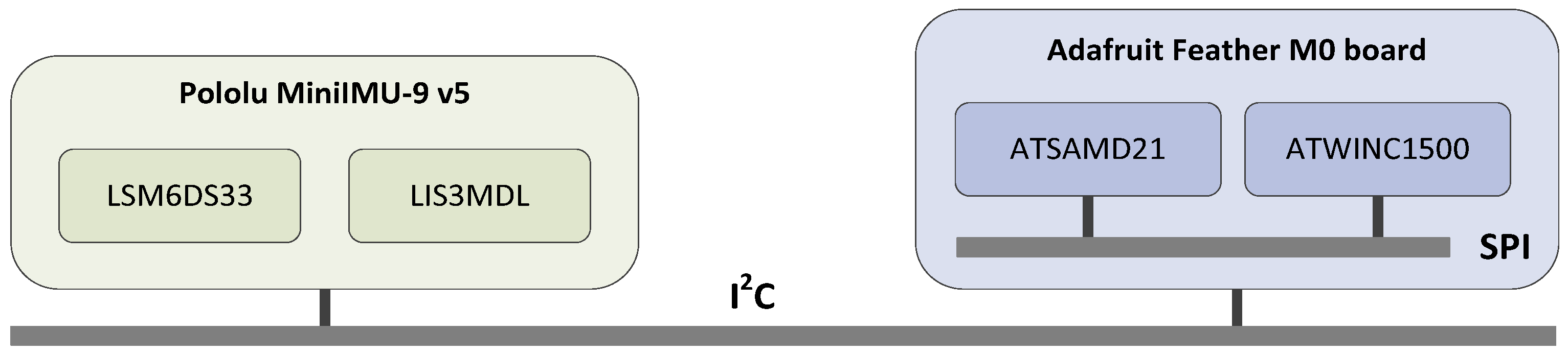
In order to meet the requirements of being lightweight and autonomous, we chose the Adafruit Feather M0 board (Adafruit, New York, NY, USA), which features an ATSAMD21 microcontroller and ATWINC1500 network controller, as a base of our system. The compact size and weight of the board make it unobtrusive to the wearer’s movement, and it can be mounted discreetly.

2.1. System Architecture and Implementation

To acquire comprehensive motion data, we utilized the MinIMU-9 v5 board (Pololu Corporation, Las Vegas, NV, USA) [8], which integrates two sensor chips manufactured by STMicroelectronics: the LIS3MDL magnetometer [19] and the LSM6DS33 accelerometer and gyroscope [20]. Together, these sensors provide measurements along three axes each, totaling nine degrees of freedom essential for detailed analysis of human movement. Sensors with more degrees of freedom can capture more detailed and precise data about movements, ensuring greater accuracy and precision. This can be beneficial for detailed analysis, but may require advanced algorithms and computing power to effectively process and interpret the data. The sensor assembly was connected to the Adafruit Feather M0 microcontroller board via the I2C communication interface, as shown in Figure 1. For our initial testing phase, we employed the Arduino IDE 2.0 with the library supplied by Pololu to configure the sensors and retrieve raw data outputs.
We utilized Pololu’s Arduino library to maintain compatibility with the Arduino environment, but for effective debugging, a more advanced Integrated Development Environment (such as a Cmake 4.0.2 project in Visual Studio Code 1.100.2 using the Cortex-Debug extension) is necessary.
In Figure 2, we present three examples of system implementations that we use in various biofeedback applications developed in our laboratory [21]. These are prototypes that will later be built into different enclosures and used as 9 DoF wearable devices with wireless communication. These are some of the devices used in the tests and measurements presented in later sections of this article.

2.2. Scheduler Implementation

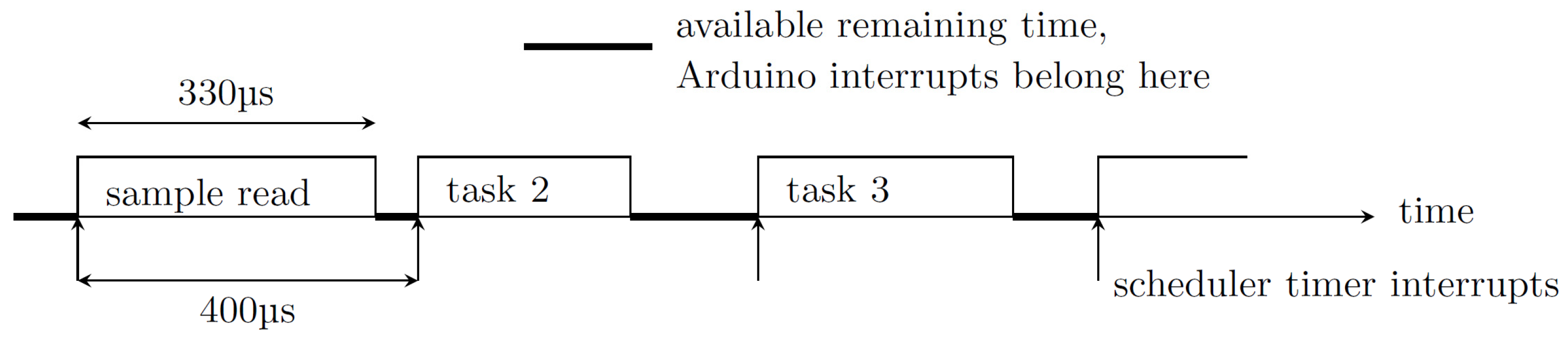
To achieve uniformly spaced sensor readings, we developed a custom cooperative periodic scheduler without task prioritization. This scheduler employs a round-robin execution model capable of handling a variable number of finite tasks, each of which must be completed within a predefined time slice. By utilizing a modular and transparent software architecture, our system prevents race conditions and CPU starvation through cooperative task scheduling without priorities. This implementation leverages a single timer interrupt, as illustrated in Figure 3. As shown in the figure, the system masks native Arduino interrupts during the execution of the timer interrupt and permits them only between the scheduled tasks.
By imposing stringent constraints on the tasks supported by our system, we were able to simplify it to its bare minimum. As shown in Figure 3, tasks are executed in a strict round-robin fashion, and it is the user’s responsibility to ensure that each task completes before the next timer interrupt occurs. Upon each interrupt, the scheduler simply retrieves the address of the next task to be executed and runs it. This approach imposes only about 3 μs of overhead, which is significantly lower than the overhead imposed by any of the RTOS solutions mentioned in the Introduction. For comparison, lightweight RTOS solutions such as FreeRTOS typically incur a task switch overhead ranging from 5 to 15 µs on ARM Cortex-M microcontrollers, with much higher delays on less capable platforms.
Due to the deterministic nature of task execution, no conflicts or unexpected task delays were observed under normal operation, as long as each task adhered to its allocated time slice. This approach not only reduces the system complexity but also eliminates the need for additional fault tolerance mechanisms such as watchdog timers, as the risk of unanticipated system hangs or deadlocks is inherently minimized by design. The primary challenge arises in high-load scenarios where a transmitted packet is not successfully received due to network conditions or interference. This, however, is not a limitation of the scheduler itself; rather, it is handled at the communication protocol level, where the system simply requests a packet resend as needed. This ensures that data transmission remains reliable without disrupting the strict timing requirements of the real-time biofeedback process.
As a direct consequence of the aforementioned simplification and overhead reduction, we were able to utilize a less powerful, energy-efficient microcontroller without compromising real-time performance. This design choice inherently contributes to lower power consumption, as the selected processor operates with reduced computational demands. (Although the expected average power draw of the selected ATSAMD21 controller is quite low (approximately 3 mA in active mode), certain other low-power models, such as the STM32L4 series, can achieve even lower active mode currents. However, these models are typically two to three times more expensive.) Additionally, the scheduler itself occupies less than 1 kB of the 256 kB of available flash memory, and its RAM usage is limited to just a few tens of bytes, primarily for maintaining task pointers and context, leaving sufficient capacity for the remaining program code and future extensions. In contrast, systems like FreeRTOS typically require 5 to 10 kB of flash memory and at least hundreds of bytes of RAM for task management and scheduling, even in their most basic configurations. The SRAM utilization in our system is similarly low, as this memory primarily serves as a buffer for sensor readings prior to transmission via the Wi-Fi interface. Since data are transmitted continuously with minimal buffering, the required SRAM remains well below 1 kB.
The selected microcontroller board (Adafruit Feather M0) is available at a unit price of approximately USD 20, while the IMU sensor module (Pololu MinIMU-9 v5) costs around USD 30, based on purchases in small quantities (fewer than 10 units). This brings the total hardware cost of the prototype system to approximately USD 50, excluding housing and power supply. The affordability of these components—even at low-volume pricing—combined with the efficiency of the proposed software architecture, underscores the potential for scalable and cost-effective deployment in industrial or consumer applications.

2.3. Preliminary Tests

Preliminary tests indicate that the minimum feasible time slice is constrained by the duration of a single raw data reading, which is approximately 330 μs for one nine-degrees-of-freedom data sample. Assuming no additional tasks are executed, the maximum achievable sampling rate is 3000 samples per second, given that the scheduler’s overhead is approximately 1% (i.e., 3 μs per cycle). With a time slice of 400 μs, a stable sampling rate of 2500 samples per second can be achieved when no other tasks are running.
To demonstrate proof of concept, we established a continuous data stream via a Universal Asynchronous Receiver-Transmitter (UART) connection through a Universal Serial Bus (USB) to a personal computer. The UART interface was chosen because the terminal software used for testing supports this type of communication. It is important to emphasize that this connection was used solely for testing purposes—to verify that the data were transmitted correctly—and is not part of the final implementation. The conversion from UART to USB was handled by a dedicated interrupt routine within the Arduino software framework. To prevent interference with real-time tasks, we assigned the routine a lower priority than the scheduler’s timer interrupt.
We successfully maintained a continuous data stream at 2500 sample packages per second. Each sample contains an 8-byte synchronization header, a 4-byte timestamp, a 4-byte sample number, and three 3D sensor vectors (magnetometer, accelerometer, and gyroscope). Each vector component is stored as a 16-bit integer, resulting in a gross sample package size of 34 bytes.

2.4. System Operation

The wearable device we designed primarily functions in a streaming mode, continuously capturing sensor data and wirelessly transmitting it to the processing unit of the RTBF system. To ensure smooth and efficient streaming, several tasks must be executed in a specific sequence:
  • Sensor Data Acquisition—Collect readings from the three sensors integrated on Pololu’s MinIMU-9 v5 board.
  • Data Formatting—Convert the raw sensor values into a format compatible with the UDP transport protocol.
  • Packet Assembly—Compile the formatted data into packets containing one or more sensor samples.
  • Data Transmission—Send the assembled packets to the processing unit via the Wi-Fi controller.
Ensuring that sensor data acquisition occurs at uniform time intervals is critical for accurate data representation. We achieve this by embedding the sampling task within the timer interrupt routine of our periodic scheduler. This routine is triggered at precise times defined by n · T s , where n is the sample index and T s is the sampling period. This setup ensures a consistent sampling frequency of f s = 1 / T s .
The Data Formatting step involves converting the sensor readings and timestamps—originally represented as unsigned 16-bit or 32-bit integers—into ASCII-encoded decimal or hexadecimal values. This conversion is required by the UDP protocol used in the microcontroller’s IP stack library. In practice, this step is often integrated with the packet assembly process.
During Packet Assembly, the formatted sensor data are combined with control data and metadata, such as sensor identifiers, timestamps, and sample numbers. Each packet may contain multiple sensor samples collected over consecutive sampling intervals.
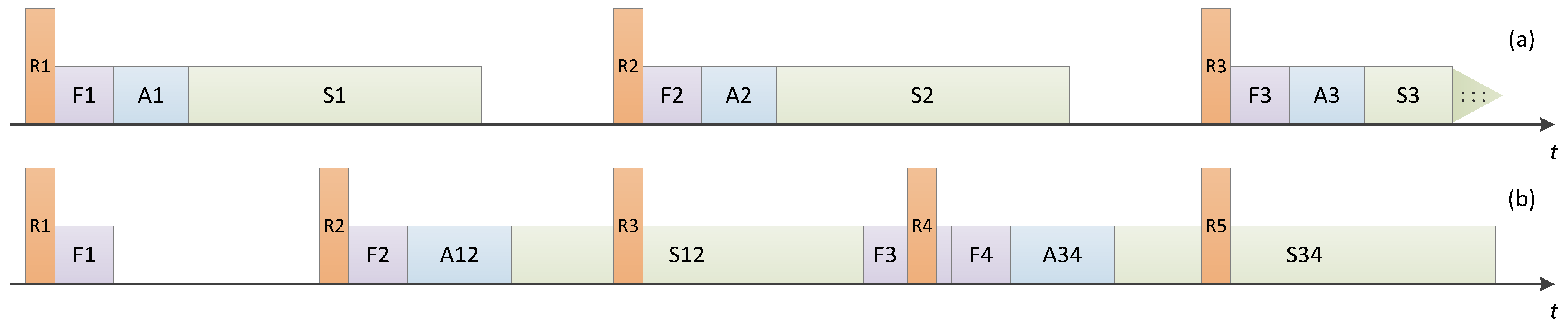
The final step, Data Transmission, involves sending the assembled packet to the ATWINC1500 Wi-Fi controller through the SPI interface on the Feather M0 board, as illustrated in Figure 1. Depending on various parameters such as sampling frequency and I2C bus speed, the system operates in one of two modes: Single-Sample Mode—each streaming packet contains a single sensor sample. All tasks must be executed within the sampling period ( T s ), as shown in Figure 4a. Multi-Sample Mode—Each streaming packet contains multiple sensor samples, usually spanning several sampling periods (e.g., S12 or F3 in Figure 4b). It can be observed that the formatting task is executed as soon as possible after each sensor sample is read. The assembly and transmission tasks are executed only after all expected sensor samples have been read and formatted. For example, in Figure 4b, samples 1 and 2 are assembled and sent together.

2.5. Measurement Methodology

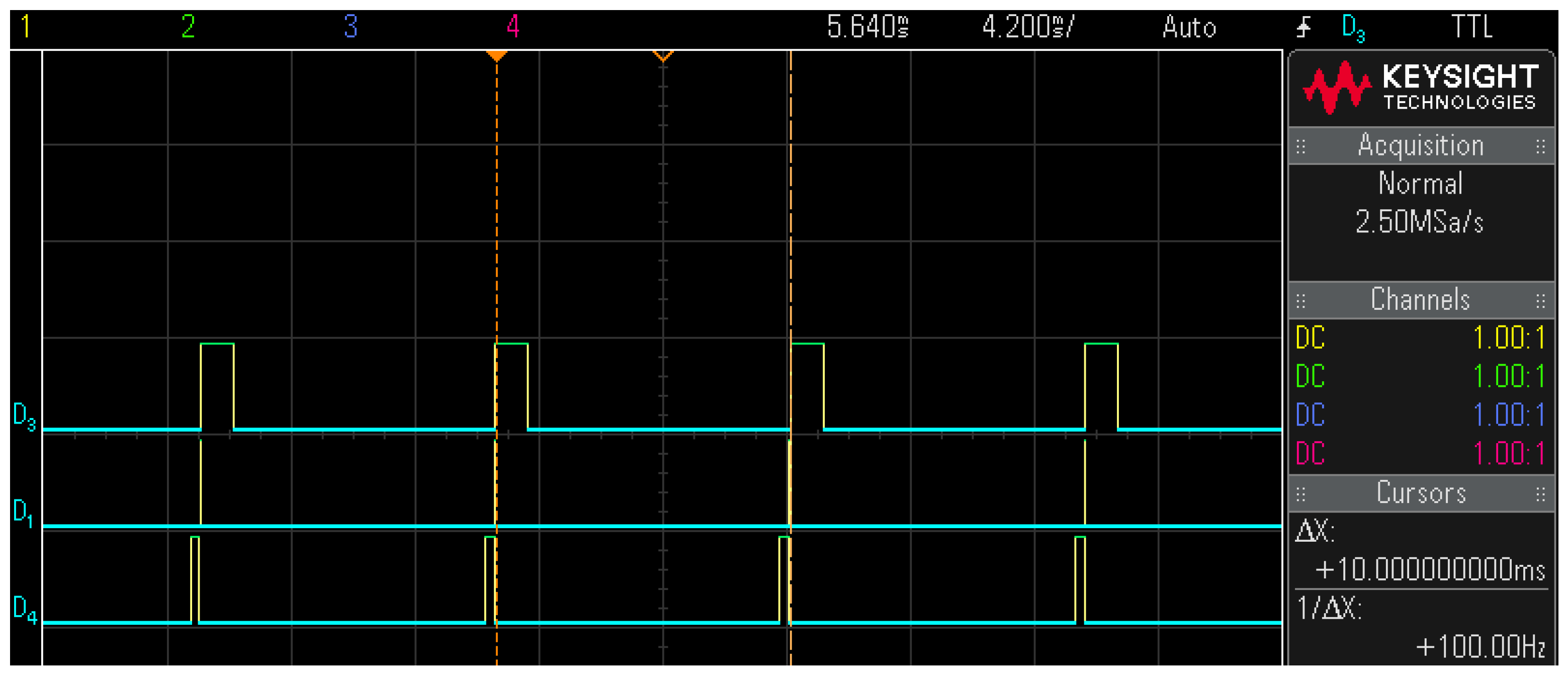
We carried out extensive measurements to record the results. For each measurement, we first checked the correct operation of the scheduler by monitoring the pin states of the microcontroller board with the oscilloscope, as described in Section 3.1. Once we had established the correct operation of the system, we carried out various measurements of the parameters that are the subject of this article.
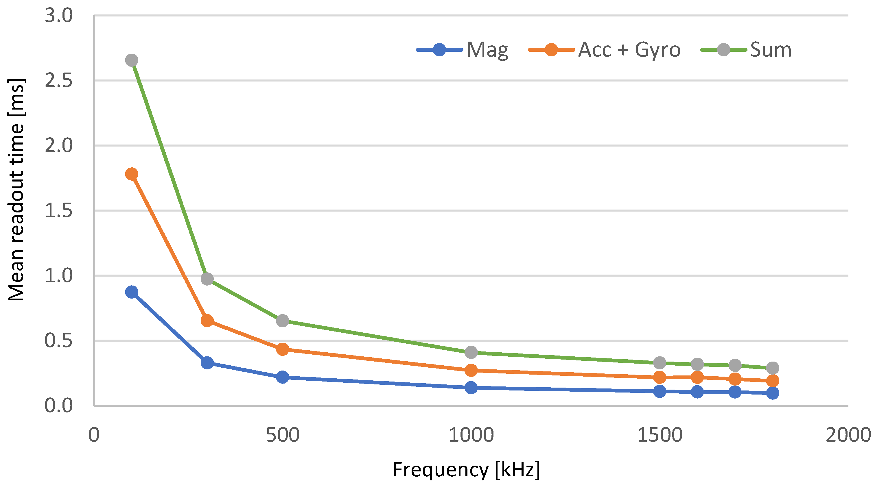
The first measurement phase was dedicated to measuring the sensor readout times at different I2C bus frequencies. Its main purpose was to determine the stable operating frequency of the I2C bus based on the results shown later in Table 1. As a result of these measurements, we used the stable I2C bus frequency of 1500 kHz for all subsequent tests, as described in more detail in Section 3.2.
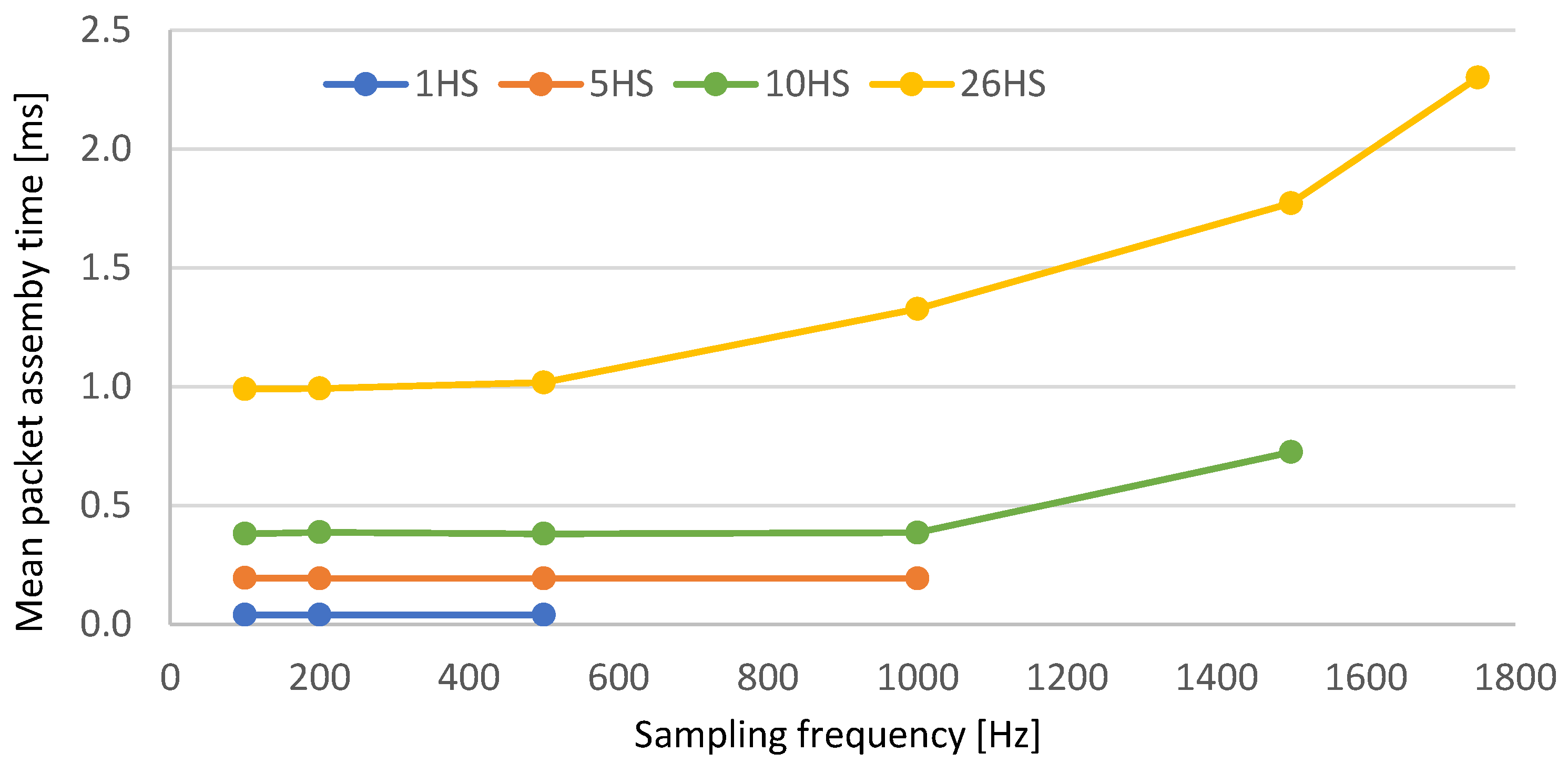
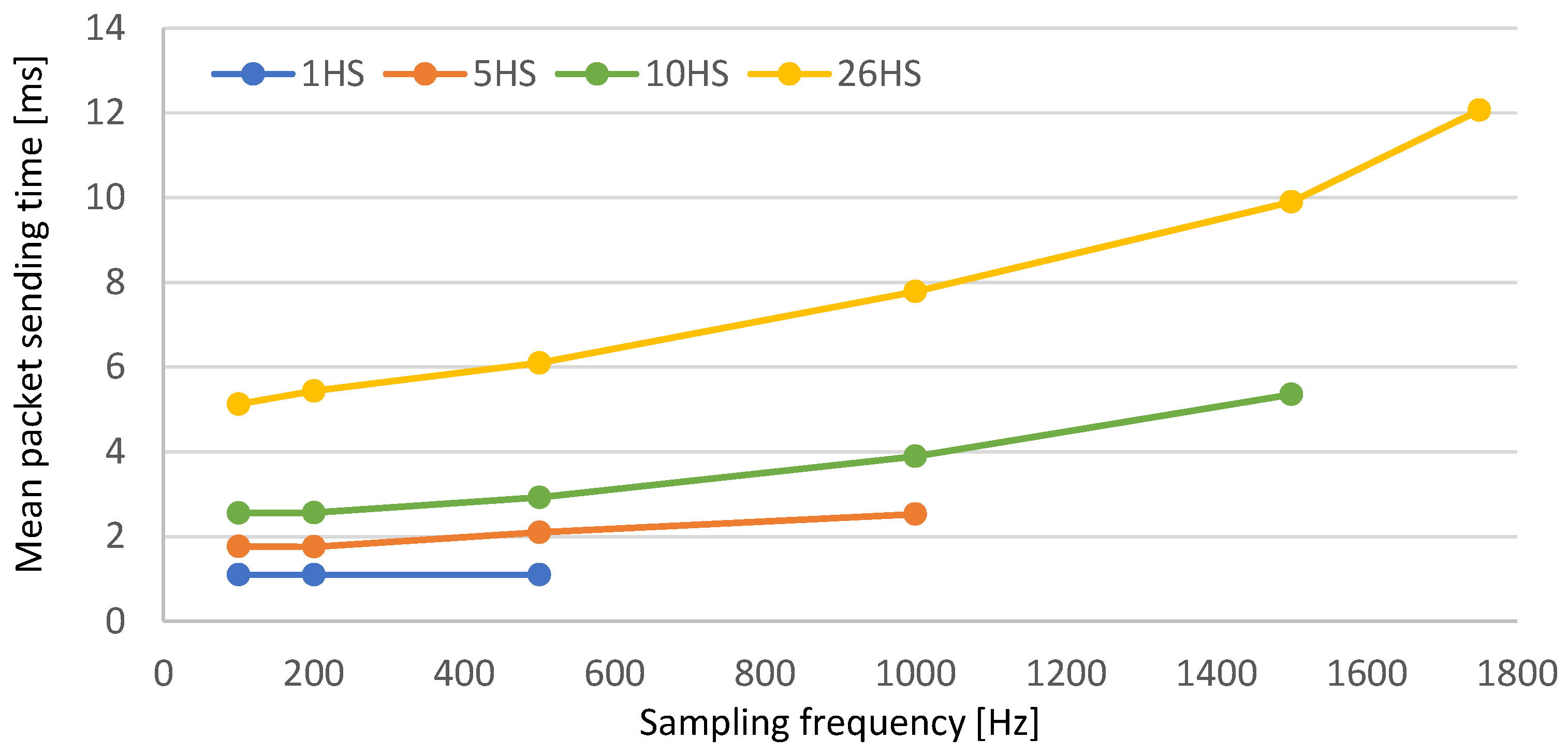
In the second phase, we used the stable I2C bus frequency of 1500 kHz for all measurements in which we determined the times for assembling and sending packets for a variety of combinations of single/multi-sensor sample streaming modes. It must be noted that we included the time for formatting the sensor samples as part of the packet assembly time (see Figure 4). We tested scenarios with 1 or more (2, 5, 10, 26) sensor samples in one packet. We also made code optimizations to speed up the execution of the tasks and achieve better results, i.e., we replaced the decimal ASCII representation of 16- or 32-bit integer values for packet assembly with the hexadecimal representation computed by two different functions. The results and comparisons are given in Section 3.3.
Finally, we measured the packet delay and its variations in the remote processing device (receiver) connected over the WiFi to our wearable device, although this was not our primary objective in this research. This issue needs to be further investigated with measurements in different environments and with a number of different commercial WiFi devices. See Section 3.4 for the results.

3. Results

It is now time to address the central research question of this work, which aims to determine the maximum sensor sampling frequency supported by a particular wearable device in streaming mode. To obtain the results, we used four different wearable devices with the architecture presented in Figure 1 and followed the methodology described in Section 2.5.

3.1. Verification of Scheduler Operation

To validate the proper operation of our scheduler, we monitored the state changes of specific pins on the Feather M0 microcontroller board by toggling them between LOW and HIGH states. At the start of each task—namely, sensor reading, packet assembly, and data transmission—the corresponding pin was set to HIGH, reverting to LOW upon task completion. Each task was assigned a dedicated pin, allowing simultaneous measurement of all pins using an oscilloscope. It is important to note again that in all measurements, the data formatting task was incorporated into the packet assembly task.
A Single-Sample Mode, where each streamed packet contains a single sensor sample, is presented in Figure 5. It illustrates four sensor sampling intervals of the system operating at a sampling frequency of 100 Hz (one sample per packet). The graph displays sampling intervals, with a measured period X of 10 milliseconds between the vertical dotted lines. This results in a sampling frequency of 1 / X = 100   H z , confirming the correct timing set by the scheduler’s timer interrupt. The oscilloscope traces show the signals at the three monitored pins: the lower trace (pin D4) corresponds to the sensor reading task that occurs at each sensor sampling period, the middle trace (pin D1) corresponds to the packet assembly task, and the upper trace (pin D3) corresponds to the packet sending task. The traces demonstrate that tasks are executed sequentially without time gaps and that all tasks are executed within one sampling period. This particular configuration also provides the microcontroller with sufficient time to perform additional tasks between the end of a sending task and the start of the next reading task, if required.
A Multi-Sample Mode, where each streamed packet contains multiple sensor samples, is shown in Figure 6. In this case, the system operates at a sampling frequency of 1750 Hz and with 26 samples per packet. It can be seen from the traces that the tasks of packet assembly (pin D3) and sending (pin D4) span several sampling periods (pin D1). Without our scheduler, executing these tasks within the short sampling period of 0.571 ms, which corresponds to the sampling frequency of 1750 Hz, would not be feasible. However, the figure confirms the correct operation of the system in multi-sample streaming mode. It is worth noting that between two consecutive packet assembly tasks (pin D3), there are 26 sensor reading tasks (pin D1 transitions), so the sampling frequency can be calculated based on the time interval and the number of reads. The main difference between the single- and multi-sample streaming modes (shown in Figure 5 and Figure 6) is that, in the first case, all the required tasks are performed within one sampling period, while in the second case, they span several sampling periods, and the scheduler must ensure correct sensor sampling throughout.
While Figure 5 and Figure 6 graphically verify the operation of our scheduler, further validation can be performed by analysing the measured times for reading the sensors, assembling the packets, and sending the packets, which are given as results in the following sections. For example, if device D operates at a sampling frequency of 1750 Hz, contains 26 samples per packet, and uses the bit-shifted hexadecimal representation, the time to read a single sample is 0.317 ms (see Table 1), the time to assemble 26 samples into a packet is 2.300 ms, and the time to send the packet is 12.060 ms (what is explained later in Section 3.3 and presented in Table 2). The total time of the above tasks is 14.677 ms, which is shorter than the cumulative duration of 26 sampling periods at 1750 Hz, which is 14.857 ms. This confirms that the system operates within the required time constraints.

3.2. Sensor Sample Reading Times and I2C Bus Frequencies

In the first measurement phase, we aimed to determine how the read times of the sensors depend on the speed of the I2C bus, which is defined by the clock frequency, and to identify the maximum stable frequency of the I2C interface for each tested device.
We performed a series of measurements of sensor read times at I2C frequencies ranging from 100 kHz to 2000 kHz. We measured each device five times at each bus frequency. As this phase is used solely to determine the stable bus frequency, we believe that no further measurements are required. Table 1 lists the mean cumulative sensor read times for four different devices at I2C bus frequencies from 100 to 1800 kHz. Attempts to operate at 2000 kHz were unsuccessful for all devices. Figure 7 illustrates the mean sensor readout times of all devices as a function of the I2C bus frequency, shown separately for the magnetometer (LIS3MDL) and the combined accelerometer and gyroscope sensor (LSM6DS33). On the Pololu MinIMU-9 v5 board, the accelerometer and gyroscope are integrated in a single chip, while the magnetometer is a separate component. Therefore, we report a combined read time for the accelerometer and gyroscope as they are read simultaneously. We do not show standard deviation results, as they fall within a few percent of the mean values and would not be visually distinguishable in the graph.
It can be seen from Table 1 and Figure 7 that higher I2C bus frequencies reduce read times and indicate stable bus operation up to 1600 kHz. To ensure reliability, we selected an I2C bus frequency of 1500 kHz for all subsequent tests. (For both critical parameters (i.e., reliable I2C bus frequency at 1500 kHz and maximum sampling frequency in Section 3.3), we observed 20 out of 20 successful trials, which corresponds to a 95% Clopper–Pearson confidence interval lower bound of approximately 0.83, indicating reasonable reliability despite the small sample size. We believe the results remain meaningful for two main reasons. First, they provide practical guidelines for developers of similar low-cost, self-made systems. Second, they establish a conservative lower bound on achievable performance, which is especially relevant when considering higher-quality, industrial-grade manufacturing).
Table 1. Mean sensor reading times (cumulative for magnetometer, accelerometer, and gyroscope) for four devices at varying I2C bus frequencies. N/A marks indicate that the communication was unstable for the device at that particular frequency.
Mean Cumulative Sensor Read Time [ms]
fwire [kHz]Device ADevice BDevice CDevice D
1002.6402.6802.6502.640
3000.9721.0040.9760.972
5000.6420.6760.6460.640
10000.3970.4320.4040.397
15000.3170.3500.3220.317
16000.3050.3380.3130.306
17000.2960.330N/A0.297
18000.286N/AN/A0.286
The I2C bus frequency is a critical parameter defined within a range of 100 to 3400 kHz. As shown in Table 1, the highest bus frequency achieved was 1800 kHz with Devices A and D, resulting in a sensor reading time of 0.286 ms. With improved device assembly and optimization, attaining even higher bus frequencies and lower sensor reading times is feasible, enabling increased sampling frequencies for the wearable device.

3.3. Packet Asesembling and Sending Times

In the second phase of our experiments, we measured the time required to assemble packets and send them to the Wi-Fi module via the SPI bus (see Figure 1 and Figure 4). The tests were conducted by incrementally increasing the sensor sampling frequency to predefined values of 100, 200, 500, 1000, 1500, and 2000 Hz, which are some of the common frequencies used in applications. If a device failed to function correctly at any of these frequencies, we decreased the frequency in steps of 50 Hz to determine the highest stable sensor sampling frequency. It is important to note that the sensor sampling frequency in this phase should not be confused with the I2C bus frequency discussed in Section 3.2.
The main results of these measurements are presented in Table 2. It lists the maximum sampling frequency achieved, and the mean times for packet assembly and sending packets across all four tested wearable devices. The data are shown for different numbers of sensor samples per packet, assembled in three different ASCII formats. We performed five measurements for each combination of the independent parameters, which are sampling frequency, number of samples in a packet, and ASCII representation of the values on each of the four devices. This means that for all the results presented in this section, we had twenty measurements from which we calculated the means and standard deviations. We would like to emphasize that the results presented in Table 2 show the maximum achieved sampling frequency that answers our research question, but these are not necessarily the sampling frequencies normally used in applications.
Table 2. Maximal achieved sampling frequency, mean times with their standard deviation for assembling, and sending packets at different number of samples in one packet in three different formats. A number in row represents the number of samples and letters the ASCII format used to represent values: D = decimal, H = hexadecimal, HS = hexadecimal calculated by a bit-shift operation.
Assembly Time [ms]Send Time [ms]
FormatMax fs [Hz]MeanSTDMeanSTD
1D4500.4580.0021.3600.001
2D5500.9180.0082.2530.013
5D6502.6400.0144.4350.050
10D6505.6250.0268.5500.075
1H6000.1270.0011.1240.002
5H11500.9530.0082.9350.005
10H13001.8900.0205.4300.010
26H13005.5000.04214.0800.031
1HS6500.0400.0051.1070.009
5HS13500.1950.0053.1000.005
10HS15500.7130.0025.2110.001
26HS17502.3000.00712.0600.035
Table 2 clearly shows the differences resulting from the different functions and formats used to calculate and represent the measured 16-bit and 32-bit integer values in ASCII format, as required by the UDP protocol in the Arduino library. We employed two data formats—decimal and hexadecimal—and utilized three different functions for converting integer values to ASCII format. The values shown in the upper part of the table correspond to the decimal ASCII representation, while the values in the middle and lower part of the table represent hexadecimal ASCII formats. The decimal conversion (indicated by D) was performed using Arduino’s built-in snprintf() function. For the hexadecimal conversion, we used custom-developed functions: the basic function decToHexMeasurements() (indicated by H) and the optimized function konvHex16() (indicated by HS).
The decimal representation of the sensor values is not optimal, but it is very useful for the prototypes, and first tests, and sufficient for all applications with low sampling frequency. Using the hexadecimal representation results in shorter packets for the same number of samples compared to the decimal representation. In the decimal representation, 1, 2, 5, and 10 samples in a packet result in a payload size of 138, 276, 690, and 1380 bytes, respectively. In hexadecimal representation, 1, 5, 10, and 26 samples in a packet result in a payload size of 53, 265, 530, and 1378 bytes, respectively.
Table 2 contains the most important results but omits some potentially interesting details. Below, we present more detailed results for the decimal number representation (D) and the hexadecimal number representation with bit-shift (HS), which is the better-performing of the two hexadecimal versions. To maintain readability, we have not included all measurement results in the manuscript. However, the complete dataset is available upon request.
Table 3 shows the mean packet assembly time with its standard deviation (it can be observed that the standard deviation of our results is small, in the range of a few percent of the mean values. It occurs for two main reasons: (a) differences in central frequencies of low-quality oscillator of the microcontroller boards, (b) inaccuracies of manual reading of oscilloscope measurement results) and Table 4 shows the mean packet send times with its standard deviation for different sensor sampling frequencies and different numbers of samples per packet using the decimal number representation. Although this format is less efficient than the hexadecimal alternative, it is very useful for rapid prototyping and low-demand wearable sensor systems—particularly in scenarios when low sampling frequencies are sufficient. Our measurements show that, using the decimal format, it is possible to send up to 10 sensor samples per packet, with maximum achievable sampling frequencies of 450 Hz, 550 Hz, and 650 Hz for 1, 2, and 5/10 samples per packet, respectively.
In high-demand wearable sensor systems, we have to use the hexadecimal representation. Figure 8 and Figure 9 present a comparative analysis of mean packet assembly and transmission times when using an optimized hexadecimal representation with bit-shifting techniques. We do not show the results of the standard deviation as they are in the range of a few percent of the mean values and would not stand out in the graph.
The results in Figure 8 and Figure 9 demonstrate that, at a constant sampling frequency, both assembly and send times increase as the number of samples per packet grows. This outcome is expected because the microcontroller must accumulate the specified number of samples before it can execute the assembly and send processes. The more samples that need to be accumulated, the more time is required for these tasks. For example, at sampling frequencies of 100 Hz and 1750 Hz, the assembly times are 0.040 ms and 0.990 ms, respectively. Similarly, with the same number of samples per packet, the assembly and send times increase with increasing sampling frequency (except in the case of one sample per packet). This behavior is due to the operation of the scheduler, where the assembly and send tasks are interrupted at each sampling interval by the sensor reading tasks (see Figure 4 and Figure 6). Although the additional time required for these tasks is not ideal, it enables the system to operate at higher sampling frequencies. For instance, when packets contain only one sample, the maximum achievable sampling frequency is limited to 500 Hz. In contrast, by including 26 samples in each packet, the system can reach sampling frequencies up to 1750 Hz.
It is worth noting that in all the results in Table 3 and Table 4 and Figure 8, Figure 9 and Figure 10, the values and curves corresponding to the scenarios with one sensor sample in a packet closely resemble the results that would be obtained with a system with the same architecture, but without our scheduler and methodology. In such systems, only one sample per packet is a viable option.
In Figure 10, we compare the mean time to perform all the tasks required to process (stream) a packet. This includes reading one, five, ten, or 26 sensor samples, assembling the samples into a packet, and sending the packet. The packet processing time increases with both the number of samples per packet and the sampling frequency, as shown previously in Figure 4 and Figure 6, and decreases with the use of more efficient value representation—from decimal to hexadecimal, and further to hexadecimal with bit-shift, as illustrated in Table 2 and Figure 10.
The relationships between assembly and send times in terms of the number of sensor samples per packet or the sampling frequency were already discussed in connection with Figure 4 and Figure 6. Analysis of Table 2 and Figure 10 shows that the transition from decimal to hexadecimal value representation significantly increases the achievable sampling frequency. This improvement is due to the ability to include more samples per packet and reduce processing times for data formatting (compare the blue lines (D) with the red (H) and green lines (HS) in Figure 10). Further optimization of the formatting of 16-bit and 32-bit integers into hexadecimal ASCII representation results in an additional reduction in processing time (compare the red (H) and green lines (HS) in Figure 10).

3.4. Packet Delay at the Receiver

In the third phase of our testing, we measured packet delays at the receiving end to evaluate the system’s performance under different conditions. As already mentioned in Section 2.5, this was not the primary objective in this research. This issue needs to be further investigated with measurements in different environments and with a number of different commercial WiFi devices. The initial results, based on measuring 1000 packets at the receiver for each point in the graph in Figure 11, indicate that the mean packet delay increases proportionally with the number of samples included in each packet. Although the jitter—calculated as the standard deviation of the delay—also rises with the number of samples, its rate of increase is significantly lower compared to that of the mean delay. Figure 11 illustrates these findings for a sampling frequency of 100 Hz and hexadecimal representation with bit-shifting.

4. Discussion

In this study, we conducted comprehensive tests using wearable devices specifically assembled for research in various biomechanical applications within sports and physical rehabilitation [22]. These applications span a wide range of actions with differing requirements: some necessitate low sampling frequencies and minimal streaming latency, while others demand high temporal resolution (i.e., high sampling frequencies) and can tolerate greater latency [16]. This section discusses factors that could enhance the performance and usability of the presented systems.
It should be reiterated that the primary research objective of this study is the maximum sensor sampling frequency that can be supported by a given wearable device in streaming mode [3]. For this reason, we did not take any measures to mitigate packet loss in the wireless Wi-Fi connection. Some RTBF applications are highly insensitive to packet loss and do not require any measures to mitigate this loss. For applications that require reliable data transmission, additional tasks need to be implemented on the wearable device, lowering the highest achievable sampling frequency determined in our experiments. The reduction depends on the complexity of the data loss mitigation measures and protocols, but the detailed study of these measures is outside the scope of this paper.
In this study, we did not consider the possible differences between the output rates of the sensor data and the sampling frequency of the device. While the former is a property of the sensor [19,20] and is controlled by its registers, the latter depends on the settings of the periodic scheduler. For our results, it does not matter if there is a discrepancy between the two, as we only measure the capabilities of the wearable device, which depend on its sampling frequency. For real applications, the output data rate of the sensor and the sampling frequency of the device must be adjusted and set correctly.
Optimizing the representation of sensor sample values in ASCII format for the UDP protocol is also crucial. By reducing the number of characters required for data representation, we increased the number of sensor samples that can be included in a single packet. The Wi-Fi protocol standard imposes a payload limit of approximately 1500 bytes, including IP and UDP headers. Considering these constraints, two options are available: (a) a decimal representation requires 138 bytes per sample and allows a maximum of 10 samples per packet and (b) a hexadecimal representation requires 53 bytes per sensor sample; therefore, a packet can hold up to 26 samples. Decimal representations are suitable for simple applications with low sampling frequencies of up to a few hundred hertz. Hexadecimal representations are required for demanding applications with high sampling frequencies or applications with additional processing load on the microcontroller.
We have used UDP at the transport layer of the communication protocol stack for several reasons: it is lightweight, has low overhead, high throughput, and is very suitable for low-latency data transmission in real-time applications [23]. However, UDP is also unreliable and suffers from packet loss [24]. While the advantageous features of UDP match well with the requirements of our RTBF applications, its disadvantages may affect some of the applications. This depends on the functions and requirements of the applications. It should be noted that many RTBF applications allow some degree of packet loss, so the disadvantages do not seriously affect them. However, if the application requires reliable data transmission, mitigation measures must be taken at higher protocol levels or within the application [23,25]. Such measures inevitably require additional processing on the microcontroller, which decreases the maximum achievable performance as measured in this paper.
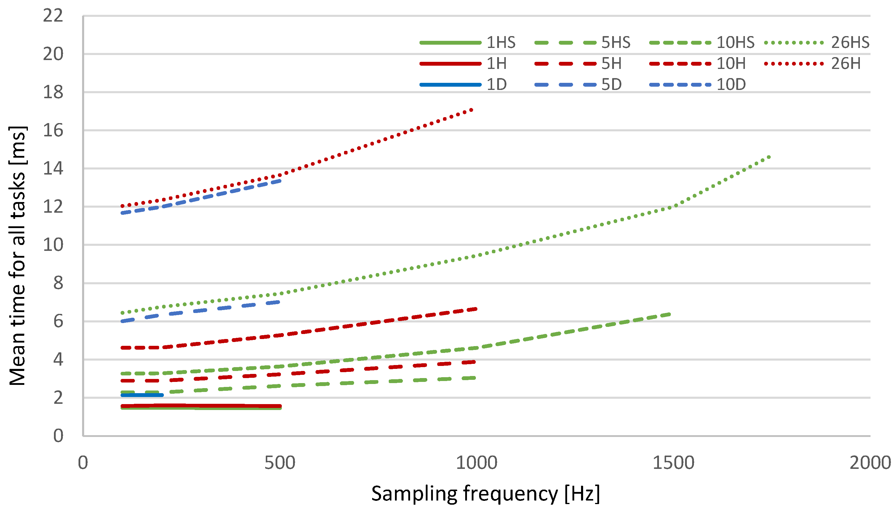
The results demonstrate that our wearable device, coupled with the developed scheduler, offers numerous combinations of sampling frequencies and packet delays, along with flexibility in payload formats. The optimal configuration depends on the specific requirements of the intended application. When assembling packets with multiple sensor samples, the packet delay at the receiver comprises the product of the number of samples and the sampling period, plus the time required to send the packet from the Wi-Fi module to the receiver (measured in milliseconds). The following three examples illustrate this.
Maximizing Sampling Frequency: To achieve the highest possible sampling frequency, the maximum number of sensor samples per packet should be used, effectively utilizing the microcontroller’s processing capacity. However, this approach results in increased packet delay at the receiver. For instance, at a sampling frequency of 1750 Hz with 26 samples per packet, the packet delay exceeds 15 ms.
Minimizing Receiver Delay: If minimizing delay at the receiver is paramount, transmitting one sample per packet is preferable. This configuration is feasible up to 650 Hz using hexadecimal representation and up to 450 Hz using decimal representation, with expected receiver delays of only a few milliseconds.
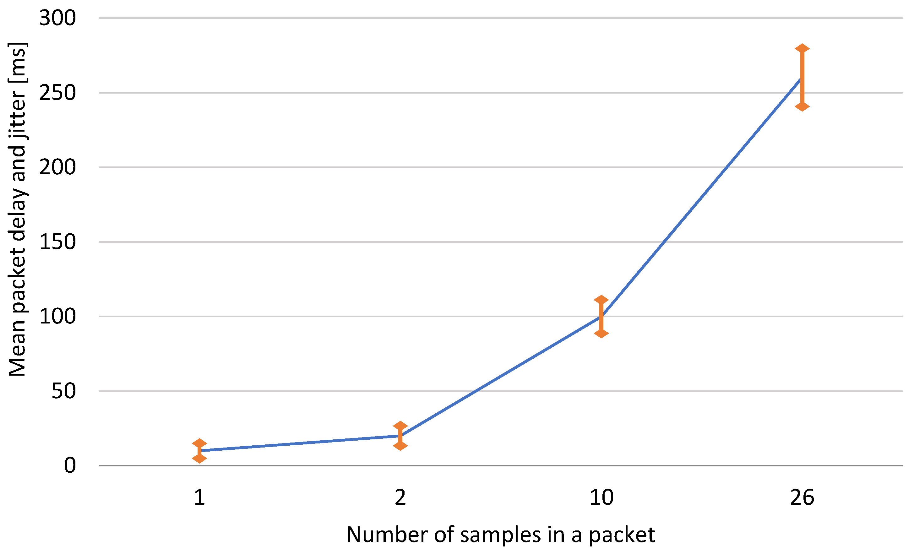
Intermediate Scenarios: Other configurations fall between these extremes. For example, as shown in Figure 11, at a sampling frequency of 100 Hz with 10 samples per packet, the receiver delay exceeds 100 ms. This is because the system must collect 10 samples (taking slightly more than 90 ms) before the packet can be transmitted. Developers of RTBF applications [16] or other systems employing such wearable devices with a scheduler now have multiple options at their disposal. In scenarios requiring maximum sampling frequencies or minimal receiver delays at the highest achievable frequencies, the microcontroller’s computing resources are almost entirely dedicated to data streaming. By avoiding these extreme cases, additional processing power remains available for other tasks unrelated to streaming, which may be necessary for the application’s successful operation [1,22].
To relate these figures to the application-specific requirements of RTBF applications, we divide them into three groups: low, medium, and high, depending on the required sampling frequency. The first group with low sampling frequency includes the streaming of motion signals with low dynamics and/or physiological parameters. An example of such an application is [18], where the sampling frequency was 64 Hz. Other examples from this group are gait and balance analysis, rehabilitation applications [2,16], and others. For this group, we can use practically any combination from Table 2. The group of medium sampling frequencies includes sports and rehabilitation applications with medium to high dynamic movements, with required frequencies from 100 Hz to 500 Hz [1]. These include various movements of the human body in different sports such as running, swimming, golf, skiing, and others [16]. For this group of applications, developers need to make a decision on the right combination of sampling frequency and number of samples in a packet, depending on the timing requirements of the application. If low delay is critical, fewer samples per packet are acceptable. For example, if the sampling frequency must be at least 500 Hz and the delay at the receiver must be less than 10 ms, we can only put five or fewer samples in a packet. The high sampling frequency group deals with frequencies above 500 Hz. Applications include human movements, often in combination with sports equipment, with very high dynamics and with impacts. Examples of such movements are skiing, ice skating, rugby, and others [16]. The aim here is to capture transient phenomena in movements that involve multiple joints or impacts of body parts and/or equipment and where the time spans are very short, sometimes less than 1 ms [7,11,15,22]. For such cases, sampling frequencies of 1000 Hz and more are required and we have to look for the solution in combinations with hexadecimal representation and multiple samples in one packet. For example, if we use 10 samples per packet and a hexadecimal representation with bit-shift, we can easily achieve a sampling frequency of 1500 Hz. This would give us a delay at the receiver of less than 10 ms.
Note that the described results represent the upper performance limit of the proposed scheduler on the current hardware configuration. Should we employ a faster processor, the scheduler’s overhead remains constant in terms of CPU cycles, meaning that its relative computational load would be lower in percentage terms, thereby increasing processing capacity. In scenarios with additional sensors or computational tasks, the feasibility of maintaining real-time performance depends primarily on the available CPU power and memory capacity. However, since the scheduler itself does not introduce complex task management overhead, it remains a lightweight and scalable solution. When increasing the sampling frequency beyond 1750 Hz, potential bottlenecks arise primarily from sensor communication limits (e.g., I2C bus speed), data formatting overhead, and wireless transmission constraints, rather than from the scheduler. Optimizing hardware components—such as using a higher-clocked processor, faster memory access, or more efficient sensor interfaces—can extend the system’s capabilities beyond the reported performance thresholds. We can assert that our findings apply to all wearable devices with similar architecture, where sensors are connected to a microcontroller and data packets are transmitted over a Wi-Fi interface. The relationships between sampling frequency, data format, and the number of samples per packet would remain consistent, with only the absolute values changing.
While our scheduler was designed specifically for real-time biomechanical feedback applications, its simplicity makes it adaptable for other real-time data collection tasks. However, unlike a full RTOS, it lacks the task management and prioritization features required for complex, multi-threaded applications such as advanced robotics or large-scale industrial automation systems with numerous concurrent processes. For simpler applications, such as continuous sensor monitoring in industrial or environmental settings, the scheduler remains a lightweight and efficient solution.

5. Conclusions

This study presents the design and validation of a lightweight periodic scheduler for microcontroller-based wearable sensor devices, aimed at enabling reliable, low-latency communication for real-time biomechanical feedback (RTBF) applications. The proposed system supports sensor sampling frequencies up to 650 Hz when transmitting one sample per packet and up to 1750 Hz when transmitting 26 samples per packet. These two values represent the extremes of system performance, while the scheduler is capable of accommodating a wide range of real-world application needs by balancing sampling frequency and data packet size.
The main contribution of this work is the demonstration that a simplified, cooperative scheduling approach can achieve real-time performance on resource-constrained devices, offering a practical and low-cost solution for RTBF systems in sports and physical rehabilitation. By minimizing computational overhead and memory usage, our scheduler allows the use of energy-efficient, low-cost hardware—making the design suitable for both prototyping and potential industrial-scale implementation.
We acknowledge that the limited sample size—five measurements on four hand-assembled systems—reduces the statistical power of our results. For instance, a 100% success rate in 20 trials corresponds to a Clopper–Pearson 95% confidence interval lower bound of approximately 0.83, which indicates encouraging, though not statistically conclusive, reliability. Nevertheless, the results offer valuable performance benchmarks and conservative estimates that practitioners can use when developing or evaluating similar systems.
Future work will focus on extending the analysis to include receiver-side performance, such as delay and jitter under varying environmental conditions, including Wi-Fi quality and frequency spectrum occupancy. We also plan to explore adaptive scheduling strategies and further optimize packet transmission protocols, particularly for more demanding multi-sensor or multi-user scenarios.

Author Contributions

All authors contributed in conceptualization, methodology, investigation, and reviewing. Writing, A.K. and I.F.; software, Á.B., M.H. and J.P.; Editing, A.U. and S.T.; visualization, A.K., M.H. and I.F.; funding acquisition, S.T. All authors have read and agreed to the published version of the manuscript.

Funding

This work is sponsored in part by the Slovenian Research and Innovation Agency within the research program ICT4QoL-Information and Communications Technologies for Quality of Life (research core funding no. P2-0246).

Institutional Review Board Statement

Not applicable.

Informed Consent Statement

Not applicable.

Data Availability Statement

The original contributions presented in this study are included in the article. Further inquiries can be directed to the corresponding author.

Acknowledgments

This article is a revised and expanded version of a conference paper [21].

Conflicts of Interest

The authors declare no conflicts of interest.

References

  1. Kos, A.; Umek, A. Biomechanical Biofeedback Systems and Applications; Springer: Berlin/Heidelberg, Germany, 2018. [Google Scholar]
  2. Giggins, O.M.; Persson, U.M.; Caulfield, B. Biofeedback in rehabilitation. J. Neuroeng. Rehabil. 2013, 10, 1–11. [Google Scholar] [CrossRef] [PubMed]
  3. Umek, A.; Kos, A. Smart equipment design challenges for real time feedback support in sport. Facta Univ. Ser. Mech. Eng. 2018, 16, 389–403. [Google Scholar] [CrossRef]
  4. Seneviratne, S.; Hu, Y.; Nguyen, T.; Lan, G.; Khalifa, S.; Thilakarathna, K.; Hassan, M.; Seneviratne, A. A Survey of Wearable Devices and Challenges. IEEE Commun. Surv. Tutor. 2017, 19, 2573–2620. [Google Scholar] [CrossRef]
  5. Aroganam, G.; Manivannan, N.; Harrison, D. Review on Wearable Technology Sensors Used in Consumer Sport Applications. Sensors 2019, 19, 1983. [Google Scholar] [CrossRef] [PubMed]
  6. Williamson, J.; Liu, Q.; Lu, F.; Mohrman, W.; Li, K.; Dick, R.; Shang, L. Data sensing and analysis: Challenges for wearables. In Proceedings of the 20th Asia and South Pacific Design Automation Conference, Tokyo, Japan, 19–22 January 2015; pp. 136–141. [Google Scholar]
  7. Lee, J.; Wheeler, K.; James, D.A. Wearable Sensors in Sport: A Practical Guide to Usage and Implementation; Springer: Singapore, 2019. [Google Scholar]
  8. Pololu’s MinIMU-9 v5 Board. Available online: https://www.pololu.com/product/2738 (accessed on 28 March 2025).
  9. McDevitt, S.; Hernandez, H.; Hicks, J.; Lowell, R.; Bentahaikt, H.; Burch, R.; Ball, J.; Chander, H.; Freeman, C.; Taylor, C.; et al. Wearables for biomechanical performance optimization and risk assessment in industrial and sports applications. Bioengineering 2022, 9, 33. [Google Scholar] [CrossRef] [PubMed]
  10. Milosevic, B.; Leardini, A.; Farella, E. Kinect and wearable inertial sensors for motor rehabilitation programs at home: State of the art and an experimental comparison. Biomed. Eng. Online 2020, 19, 25. [Google Scholar] [CrossRef] [PubMed]
  11. Lapinski, M.; Medeiros, C.B.; Scarborough, D.M.; Berkson, E.; Gill, T.J.; Kepple, T.; Paradiso, J.A. A Wide-Range, Wireless Wearable Inertial Motion Sensing System for Capturing Fast Athletic Biomechanics in Overhead Pitching. Sensors 2019, 19, 3637. [Google Scholar] [CrossRef] [PubMed]
  12. Yuan, S.; Bai, J.; Li, S.; Ma, N.; Deng, S.; Zhu, H.; Li, T.; Zhang, T. A Multifunctional and Selective Ionic Flexible Sensor with High Environmental Suitability for Tactile Perception. Adv. Funct. Mater. 2024, 34, 2309626. [Google Scholar] [CrossRef]
  13. Ou-Yang, W.; Liu, L.; Xie, M.; Zhou, S.; Hu, X.; Wu, H.; Tian, Z.; Chen, X.; Zhu, Y.; Li, J. Recent advances in triboelectric nanogenerator-based self-powered sensors for monitoring human body signals. Nano Energy 2024, 120, 109151. [Google Scholar] [CrossRef]
  14. Lanata, A.; Greco, A.; Di Modica, S.; Niccolini, F.; Vivaldi, F.; Di Francesco, F.; Tamantini, C.; Cordella, F.; Zollo, L.; Di Rienzo, M.; et al. A new smart-fabric based body area sensor network for work risk assessment. In Proceedings of the 2020 IEEE International Workshop on Metrology for Industry 4.0 & IoT, Rome Italy, 3–5 June 2020; pp. 187–190. [Google Scholar]
  15. Rana, M.; Mittal, V. Wearable sensors for real-time kinematics analysis in sports: A review. IEEE Sens. J. 2020, 21, 1187–1207. [Google Scholar] [CrossRef]
  16. Hribernik, M.; Umek, A.; Tomažič, S.; Kos, A. Review of Real-Time Biomechanical Feedback Systems in Sport and Rehabilitation. Sensors 2022, 22, 3006. [Google Scholar] [CrossRef] [PubMed]
  17. Ashapkina, M.S.; Alpatov, A.V.; Sablina, V.A.; Melnik, O.V. Vibro-Tactile Portable Device for Home-Base Physical Rehabilitation. In Proceedings of the 2021 10th Mediterranean Conference on Embedded Computing (MECO), Budva, Montenegro, 7–11 June 2021; pp. 1–4. [Google Scholar]
  18. Cheriyan, A.M.; Jarvi, A.; Kalbarczyk, Z.; Iyer, R.K.; Watkin, K.L. Pervasive real-time biomedical monitoring system. In Proceedings of the 2009 International Conference on Biomedical and Pharmaceutical Engineering, Singapore, 2–4 December 2009; pp. 1–8. [Google Scholar]
  19. LIS3MDL Datasheet. Available online: https://www.st.com/resource/en/datasheet/lis3mdl.pdf (accessed on 28 March 2025).
  20. LSM6DS33 Datasheet. Available online: https://www.st.com/resource/en/datasheet/lsm6ds3tr-c.pdf (accessed on 28 March 2025).
  21. Kos, A.; Tomažič, S.; Umek, A. Affordable Wearable Devices with Low-Latency Wireless Communication. In Proceedings of the 2023 IEEE AFRICON, Nairobi, Kenya, 20–22 September 2023; pp. 1–5. [Google Scholar]
  22. Camomilla, V.; Bergamini, E.; Fantozzi, S.; Vannozzi, G. Trends supporting the in-field use of wearable inertial sensors for sport performance evaluation: A systematic review. Sensors 2018, 18, 873. [Google Scholar] [CrossRef] [PubMed]
  23. Bekele, B.E.; Tokarz, K.; Gebeyehu, N.Y.; Pochopień, B.; Mrozek, D. Performance Evaluation of UDP-Based Data Transmission with Acknowledgment for Various Network Topologies in IoT Environments. Electronics 2024, 13, 3697. [Google Scholar] [CrossRef]
  24. AL-Dhief, F.T.; Sabri, N.; Latiff, N.A.; Malik, N.N.N.A.; Albader, M.A.A.; Mohammed, M.A.; AL-Haddad, R.N.; Salman, Y.D.; Ghani, M.K.A.; Obaid, O.I. Performance comparison between TCP and UDP protocols in different simulation scenarios. Int. J. Eng. Technol. 2018, 7, 172–176. [Google Scholar] [CrossRef]
  25. Bhattacharya, A.; Parlos, A.G. Flow Control of Real-time Multimedia Applications in Best-effort Networks. In Recent Advances in Intelligent Control Systems; Springer: London, UK, 2009; pp. 311–356. [Google Scholar]
Figure 1. Schematic representation of the connection between the sensors and the Adafruit Feather M0 microcontroller via the I2C interface. The microcontroller (ATSAMD21) communicates directly with the LIS3MDL and LSM6DS33 sensor modules.
Applsci 15 06405 g001
Figure 2. Three examples of the system implementation with Adafruit Feather M0 board with added Pololu’s MinIMU-9 v5 board and other elements such as battery or LED indicators.
Applsci 15 06405 g002
Figure 3. Implementation of a single timer interrupt serving as a periodic task scheduler.
Applsci 15 06405 g003
Figure 4. Operation of the scheduler at two different sampling frequencies and number of samples in a packet. The graph shows (a) the situation with one sensor sample in one packet, (b) the situation with two sensor samples in one packet. Labels R, F, A, and S denote reading, formatting, assembly, and sending tasks, respectively.
Applsci 15 06405 g004
Figure 5. Oscilloscope traces of four sensor sampling intervals at a 100 Hz sampling frequency with one sample per packet. The lower trace (D4) represents sensor reading tasks at sampling periods, the middle trace (D1) shows packet assembly times, and the upper trace (D3) indicates packet transmission times. The sampling time is 10 ms, as indicated by two vertical dotted lines.
Applsci 15 06405 g005
Figure 6. Oscilloscope traces of one packet sending episode at a 1750 Hz sampling frequency with 26 sensor samples per packet. The lower trace (D1) represents 26 sensor sampling periods, the middle trace (D3) shows packet assembly time, and the upper trace (D4) indicates packet transmission time. Two vertical dotted lines measure the packet assembly time of 2.3 ms.
Applsci 15 06405 g006
Figure 7. Mean sensor readout times across all devices versus I2C bus frequency for the magnetometer (Mag), accelerometer and gyroscope (Acc + Gyro) that are acquired together and their sum.
Applsci 15 06405 g007
Figure 8. Mean packet assembly times for varying numbers of samples per packet, using optimized hexadecimal representation with bit-shifting (HS). Legend label numbers denote the number of samples in one packet.
Applsci 15 06405 g008
Figure 9. Mean packet sending times for varying numbers of samples per packet, using optimized hexadecimal representation with bit-shifting (HS). Legend label numbers denote the number of samples in one packet.
Applsci 15 06405 g009
Figure 10. Mean time for completion of all tasks needed to acquire all sensor samples, assemble and send one packet, depending on the number of samples in one packet and sensor sampling frequency. Legend label numbers denote the number of samples in one packet, letters denote different sensor value representations: D = decimal, H = hexadecimal, HS = hexadecimal with a bit-shift.
Applsci 15 06405 g010
Figure 11. Mean packet delay and jitter at the receiver at sensor sampling frequency of 100 Hz. The mean delay is shown as a solid line, the jitter as a vertical bar.
Applsci 15 06405 g011
Table 3. Mean packet assembly times with their standard deviation for different sensor sampling frequencies fs and different number of samples in one packet for the decimal format. A number in column labels represents the number of samples per packet. N/A marks indicate that data collection was attempted but unsuccessful at that particular frequency. Empty cells indicate that measurements were not performed at that frequency.
Mean Assembly Time [ms]STD of Assembly Time [ms]
fs [Hz]1D2D5D10D1D2D5D10D
1000.4460.9052.2704.5250.0040.0060.0210.033
2000.4520.9012.2604.5150.0070.0050.0200.017
4500.458 0.002
500N/A0.8992.6235.220N/A0.0070.0180.047
550 0.918 0.008
600 N/A2.6035.555 N/A0.0040.017
650 N/A2.6405.625 N/A0.0140.026
700 N/AN/AN/A N/AN/AN/A
Table 4. Mean packet send times with their standard deviation for different sensor sampling frequencies fs and different number of samples in one packet for the decimal format. A number in column labels represents the number of samples per packet. N/A marks indicate that data collection was attempted but unsuccessful at that particular frequency. Empty cells indicate that measurements were not performed at that frequency.
Mean Send Time [ms]STD of Send Time [ms]
fs [Hz]1D2D5D10D1D2D5D10D
1000.4460.9052.2704.5250.0010.0040.0100.009
2000.4520.9012.2604.5150.0020.0020.0220.009
4500.458 0.001
500N/A0.8992.6235.220N/A0.0080.0430.010
550 0.918 0.013
600 N/A2.6035.555 N/A0.0450.058
650 N/A2.6405.625 N/A0.0500.075
700 N/AN/AN/A N/AN/AN/A
Disclaimer/Publisher’s Note: The statements, opinions and data contained in all publications are solely those of the individual author(s) and contributor(s) and not of MDPI and/or the editor(s). MDPI and/or the editor(s) disclaim responsibility for any injury to people or property resulting from any ideas, methods, instructions or products referred to in the content.

