Article

Chaotic Vibration Prediction of a Laminated Composite Cantilever Beam

School of Environmental and Safety Engineering, Liaoning Petrochemical University, Fushun 113001, China
*
Authors to whom correspondence should be addressed.
Appl. Sci. 2025, 15(12), 6403; https://doi.org/10.3390/app15126403
Submission received: 29 April 2025 / Revised: 2 June 2025 / Accepted: 5 June 2025 / Published: 6 June 2025

Abstract

The deep learning method of the recurrent neural network (RNN) is applied to predict the chaotic vibrations of a laminated composite cantilever beam. The RNN model converts time series data into a multi-step supervised learning format and normalizes it using MinMaxScaler. The cantilever structure is subjected to an evenly distributed load, and a series of chaotic vibrations are observed corresponding to different amplitudes and angular velocities of the load. Then, the RNN data-driven model is applied to predict chaotic vibrations, and the chaotic vibration prediction of RNN is evaluated. The prediction results are primarily evaluated using two metrics: mean absolute error (MAE) and root mean square error (RMSE). The analysis results show that the maximum MAE is 0.041 and the maximum RMSE is 0.067. Even under perturbed initial conditions, the RNN model maintained high prediction accuracy, with a maximum MAE of 0.022 and RMSE of 0.038, highlighting its robustness and reliability in predicting chaotic vibrations. The error analysis indicates that the RNN accurately predicts chaotic vibrations with a high degree of precision.

1. Introduction

Composite materials offer unique advantages, including high strength, light weight, and excellent fatigue resistance. In recent years, the application of composite materials in modern engineering has become increasingly widespread, particularly in high-performance structures such as aerospace [1,2], transportation [3], and civil engineering [4]. Because of their internal heterogeneity and complex structure, composites often exhibit pronounced nonlinear dynamic characteristics in practical applications. Under complex external loads, these materials frequently display chaotic vibrations as well as other nonlinear dynamic phenomena. As the complexity of engineering structures continues to increase, traditional theoretical and numerical methods encounter significant limitations in solving complex nonlinear dynamic problems. The rapid development of deep learning in recent years has introduced innovative approaches for tackling complex predictive challenges. Notably, deep learning models such as recurrent neural networks (RNNs), long short-term memory (LSTM), and convolutional neural networks (CNNs) have shown remarkable capability in predicting nonlinear dynamic systems. Currently, deep learning methods have been widely applied in different fields including performance prediction of diverse engineering structures [5] and weather forecasting [6,7], since data-driven models effectively predict the complex behavior of nonlinear systems. However, research on predicting chaotic vibrations of laminated composite cantilever beams remains unexplored.
Composite structures are widely applied in engineering and the emerging field of energy harvesting, and their nonlinear dynamic behavior has been studied extensively over the last decades. Early in the 2000s, Zhang et al. [8] modeled a cantilever structure as an Euler–Bernoulli beam and verified that nonlinear nonplanar vibrations of the cantilever beam can exhibit chaotic vibrations under conditions of harmonic axial excitation and lateral excitation in the free segment. Bouadjadja et al. [9] performed a theoretical analysis of large deflections of composite cantilever beams based on an Euler–Bernoulli beam and validated their findings through experiments. Cheng et al. [10] proposed a frequency-variable structure for piezoelectric vibration energy harvesting based on nonlinear magnetic force and piecewise linear force and conducted a detailed discussion on the factors affecting the proposed vibration energy harvesting device through theoretical and experimental analysis. Wu et al. [11] applied first-order shear deformation theory to study the influence of different parameters on the nonlinear dynamic behavior of low-content graphene-reinforced composite plates. Guo et al. [12] derived the multi-dimensional dynamic equation of graphene-reinforced composite cantilever structures through first-order deformation theory and analyzed the influence of nonlinear terms on the dynamic behavior of different vibration modes. Viet et al. [13] studied the nonlinear behavior of composite cantilever beams subject to concentrated loads using Timoshenko beam theory and discussed the influence of temperature and the number of composite layers on the deformation of cantilever beams. Li et al. [14] employed third-order shear deformation theory and introduced the dynamic stiffness method to investigate the influence of beam length on the free vibrations of laminated composite cantilever beams. Amabili et al. [15] proposed a refined third-order shear deformation theory for nonlinear vibrations of cantilever beams and conducted large-amplitude vibration experiments and numerical simulations on self-healing cantilever beams. Zhang et al. [16] established a two-dimensional nonlinear dynamic system of a symmetric cross-ply laminated composite cantilever structure, discussing the effects of different types of excitations on the nonlinear vibrations of the structure and discovering the presence of chaotic vibrations in the established system. Liu and Sun [17] applied the Galerkin discretization and derived a two-dimensional nonlinear system of a cantilever beam. When establishing the model, the influence of the third-order shear effects on beam vibration was considered, and the chaotic response was discovered through numerical simulation. Guo et al. [18] applied third-order shear deformation to model a cantilever macrofiber composite structure. The study found that the system would produce nonlinear vibration responses under different disturbance forces. Zhang et al. [19] studied bistable asymmetric deployable composite laminated cantilever structures and established a two-dimensional nonlinear dynamic system. They discovered that the foundation excitation amplitude and frequency may lead to chaotic snap-through vibrations of the cantilever structures. Sun et al. [20] modeled a composite laminated cantilever structure and derived a two-dimensional dynamic system considering third-order shear effects. They proved the necessity of using multi-dimensional systems for studying the vibration of composite laminated cantilever beams and controlled the limit cycle response of the structure. Ghazoul et al. [21] established a porous laminated structure model using higher-order shear deformation theory, analyzed the buckling and free vibration performance of a porous laminated functionally graded carbon nanotube reinforced composite (FG-CNTRC) structure, and discussed the effects of different parameters on the critical buckling load and the natural frequency of the porous laminated FG-CNTRC structure. Rosso et al. [22] proposed a method to enhance the nonlinear magnetic plucking of vibration energy harvesters by attaching oppositely polarized neodymium–iron–boron shielding magnets around the main magnet. Computational studies on a piezoelectric energy harvester with dual piezoelectric patches showed that this method can significantly increase the peak power. Hao et al. [23] established a nonlinear dynamic system of a graphene-reinforced functionally graded porous rotating cantilever structure and investigated the nonlinear bifurcation and chaotic behavior of the system under primary and internal resonance conditions. Thus, it is important to predict the nonlinear vibrations of a laminated composite cantilever beam to ensure the safety of such engineering structures.
As one of the fundamental deep learning methods, RNN has been applied in various fields, such as nonlinear system investigation, image recognition, and climate prediction. In the last several years, it has been applied in analyzing the nonlinear dynamics of engineering structures. In 2015, Qi et al. [24] studied the nonlinear spatiotemporal dynamics of a cantilever-based micro nanomanipulator using a radial basis function RNN, which effectively identified the model of the investigated cantilever structure. In 2019, Subramanian and Mahadevan [25] combined Bayesian state estimation with a deterministic RNN to predict the vibration of a nonlinear air cycle machine, and demonstrated the prediction process through a dynamic discrete system. At the same time, Teng and Zhang [26] proposed a new multi-step deep neural network (DNN) model by combining CNN, LSTM, and a multi-step method to identify nonlinear dynamical systems and predict their future states. The model was compared with other multi-step DNNs and showed better performance in predicting chaotic vibration dynamics. In the same year, Cestnik and Abel [27] evaluated the predictive capacity of both LSTM and the gated recurrent unit (GRU) in three chaotic systems, and both were shown to be effective in estimating the dynamic properties of nonlinear systems. In 2021, Huang et al. [28] proposed a new prediction model based on a dual-stage attention-based RNN and GRU to identify the periodicity and long-distance dependence characteristics of sequence data. In 2021, Uribarri and Mindlin [29] employed LSTM to predict chaotic time series from a Rössler system. In 2022, Dudukcu et al. [30] proposed a new temporal convolutional RNN model and validated its accuracy through different chaotic systems, including a Lorenz system and a Rössler system. In the same year, Sangiorgio et al. [31] introduced different levels of noise to chaotic systems, used different prediction models to predict the chaotic systems, and confirmed the robustness of LSTM without teacher forcing in handling complex systems and noise. In 2023, Sun et al. [32] established a five-degree-of-freedom Duffing system and proposed an LSTM encoder–decoder neural network prediction method, proving its capability in predicting chaotic vibrations in discrete systems. In the same year, Zhang et al. [33] proposed a robust RNN to reduce prediction errors, which would occur due to noise existing in real-world time series. At the same time, Khatir et al. [34] combined the particle swarm optimization (PSO) algorithm with YUKI to propose PSO-YUKI, using a radial basis function (RBF) neural network to predict the double cracking of cantilever carbon fiber-reinforced polymer (CFRP) beams. The results demonstrate that the PSO-YUKI approach has better accuracy and effectiveness in damage prediction compared to the standalone PSO method. In 2024, Khatir et al. [35] experimentally demonstrated that near-surface mounted (NSM)-strengthened beams can reduce crack loss and limit frequency changes under bending conditions. Meanwhile, PSO and genetic algorithms (GAs) were used to fine-tune the gradient boosting (GB) model. Data obtained from static tests proved that the improved GB model is more efficient and effective in predicting the reinforced concrete (RC) strain. In 2025, Wang et al. [36] proposed a data-driven model by combining CNN and convolutional LSTM, validating its accuracy and efficiency in predicting chaotic vibrations in a micro-beam system. Recently, Khatir et al. [37] used the reptile search algorithm (RSA) to optimize the artificial neural network (ANN) and proposed a hybrid ANN-RSA model. Combining experiments and numerical simulations, they demonstrated the accuracy and computational efficiency of the ANN-RSA. Osmani et al. [38] combined analytical models and ANN to propose an algorithm for predicting the deflection of variable cross-section castellated steel beams and verified the correctness of the algorithm through a finite element model. However, so far, no deep learning methods, including RNN, have been applied to predicting the chaotic vibrations of a laminated composite cantilever beam.
Traditional numerical simulation methods typically require researchers to possess extensive domain knowledge, as well as the ability to formulate and solve complex differential equations. In contrast, an RNN data-driven model bypasses the need for theoretical modeling by combining representation learning with model training, without relying on explicit physical equations or expert-derived models. The key advantage of RNN lies in its ability to implicitly capture the underlying nonlinear dynamics of complex systems. By learning temporal dependencies directly from historical input–output sequences, RNN offers a promising alternative for predicting chaotic vibrations in cases where physical models are difficult to derive or unavailable.
Therefore, it is important to test the feasibility of the RNN data-driven model for predicting chaotic vibrations of a laminated composite cantilever beam. The current structure of this work is organized as follows: In the Section 2, a multi-dimensional nonlinear dynamic system of a laminated composite cantilever beam subjected to periodic excitation is established. In the Section 3, the concept, definition, and modeling process of the RNN data-driven model is introduced. In the Section 4, numerical simulations are conducted using different amplitudes and angular velocities of the evenly distributed load, to evaluate the accuracy of the employed RNN data-driven model in predicting chaotic vibrations of the studied laminated composite cantilever beam. In the Section 5, the conclusions of the current work are drawn.

2. Beam Model Establishment

To demonstrate the feasibility of the RNN data-driven model for predicting chaotic vibrations in a multi-dimensional nonlinear dynamic system of a laminated composite cantilever beam, time-series data of chaotic vibrations are generated through numerical simulations. In this section, the multi-dimensional nonlinear dynamic model of a cantilever beam is established.
In Figure 1, a three-layer laminated composite cantilever beam is shown, and a Cartesian coordinate system o x y z is applied to describe the deformation of the beam. The cross-section of the structure is uniformly rectangular; l , b , and h represents the total length, breadth, and height of the beam, and each layer of the beam features the same length, breadth, and height; the external excitation, denoted by q , is evenly applied to the beam.
In the case of no deformation, the location of any point on the structure is as follows:
r = x i + z k ,
where i and k are the unit vectors along x and z , respectively.
Following Reddy’s third-order shear theory [39], the displacement of any point on the beam after deformation is as follows:
R = x + u 0 + z x z 3 c 1 x + w 0 x i + z + w 0 k ,
where c 1 = 4 / 3 h 2 ; u 0 and w 0 are the displacements of a point on the middle plane of the structure, and x is the curvature according to Reddy’s third-order shear theory.
According to Equations (1) and (2), the structure’s kinetic energy T [40] is obtained as follows:
T = V 1 2 ρ d R d t 2 d V ,
where ρ is the density of the structure.
Based on the von Kármán type equation [41] and Equation (2), the strains of the beam are derived below:
ε 11 = u 0 x + 1 2 w 0 x 2 + z x x c 1 z 3 x x + 2 w 0 x 2 ,
ε 13 = 1 3 c 1 z 2 x + w 0 x ,
where ε 11 and ε 13 are the strains along x and z , respectively.
From Equations (4) and (5), the potential energy of the beam U is obtained as follows:
U = V 1 2 Q 11 ε 11 ε 11 + Q 13 ε 13 ε 13 d V ,
where Q 11 and Q 13 are the elastic coefficients along x and z , respectively.
The virtual work W , due to the damping force and q , is given below:
W = b 0 l c d w 0 d t w 0 d x + b 0 l q w 0 d x ,
where
q = Q 1 sin Q 2 t ,
c is the damping coefficient, and Q 1 and Q 2 are the magnitude and angular frequency of the excitation.
Following Hamilton’s principle [42], it is obtained that
t 1 t 2 δ L + δ W d t = 0 ,
where L is given as follows:
L = T U .
With the introduction of Equations (3), (6) and (7) into Equation (9), the equations of motion of the beam are derived by following the assumption of an orthogonally symmetric laminated beam and presented in the Appendix A, and then, u 0 and x are derived by following the previous study [2]:
u 0 x = 1 2 w 0 x 2 + 1 2 l 0 l w 0 x 2 d x ,
x = w 0 x + F 11 c 1 D 11 A 55 6 D 55 c 1 + 9 F 55 c 1 2 3 w 0 x 3 .
With the introduction of Equations (11) and (12) into Equation (A1), it is obtained that
I 0 d 2 w 0 d t 2 + c 1 I 4 2 x 2 d 2 w 0 d t 2 c 1 J 4 F 11 c 1 D 11 A 55 6 D 55 c 1 + 9 F 55 c 1 2 4 x 4 d 2 w 0 d t 2 c d w 0 d t + A 11 2 l 2 w 0 x 2 0 l w 0 x 2 d x D 11 4 w 0 x 4 + c 1 F 11 c 1 H 11 F 11 c 1 D 11 A 55 6 D 55 c 1 + 9 F 55 c 1 2 6 w 0 x 6 + q = 0 .
Furthermore, the following dimensionless variables are given in order to validate Equation (13):
t ¯ = Q 11 2 I I 0 b l 4 t = τ t ,   x ¯ = x l ,   w ¯ 0 = w 0 h ,   d w ¯ 0 d t ¯ = 1 τ h d w 0 d t ,   d 2 w ¯ 0 d t ¯ 2 = 1 τ 2 h d 2 w 0 d t 2 ,   c ¯ = c / Q 11 ( 2 ) h τ ,
where I and I 0 are given in Appendix A.
With Equation (14) substituted into Equation (13), it is derived that
A d 2 w ¯ 0 d t ¯ 2 + B 2 x ¯ 2 d 2 w ¯ 0 d t ¯ 2 C 4 x ¯ 4 d 2 w ¯ 0 d t ¯ 2 D d w ¯ 0 d t ¯ + F 2 w ¯ 0 x ¯ 2 0 1 w ¯ 0 x ¯ 2 d x ¯ G 4 w ¯ 0 x ¯ 4 + H 6 w ¯ 0 x ¯ 6 + q ¯ = 0 ,
where A , B , C , D , F , G , and H are given in Appendix A. To better facilitate the expression, w ¯ 0 , x ¯ , t ¯ , and q ¯ are replaced with w 0 , x , t , and q , respectively.
Based on Galerkin discretization [8], w 0 can be given as follows:
w 0 = n = 1 φ n x w n , 1 t .
Considering the cantilever boundary conditions, φ n ( x ) is given as follows:
φ n x = c h λ n x cos λ n x c h λ n + cos λ n s h λ n + sin λ n s h λ n x sin λ n x ,
where λ 1 = 1.875 and λ 2 = 4.694 are given based on second-order Galerkin discretization. For brevity, φ n x and w n , 1 t are replaced with φ n and w n , 1 for the rest of the study.
Following second-order Galerkin discretization, the response w P at x P = 0.75 is given below:
w P = n = 1 2 φ n w n , 1 = φ 1 w 1,1 + φ 2 w 2,1 = 1.315382461 w 1,1 + 0.27008056 w 2,1 ,
where w 1,1 and w 2,1 are given in Appendix A.

3. RNN Data-Driven Model Establishment

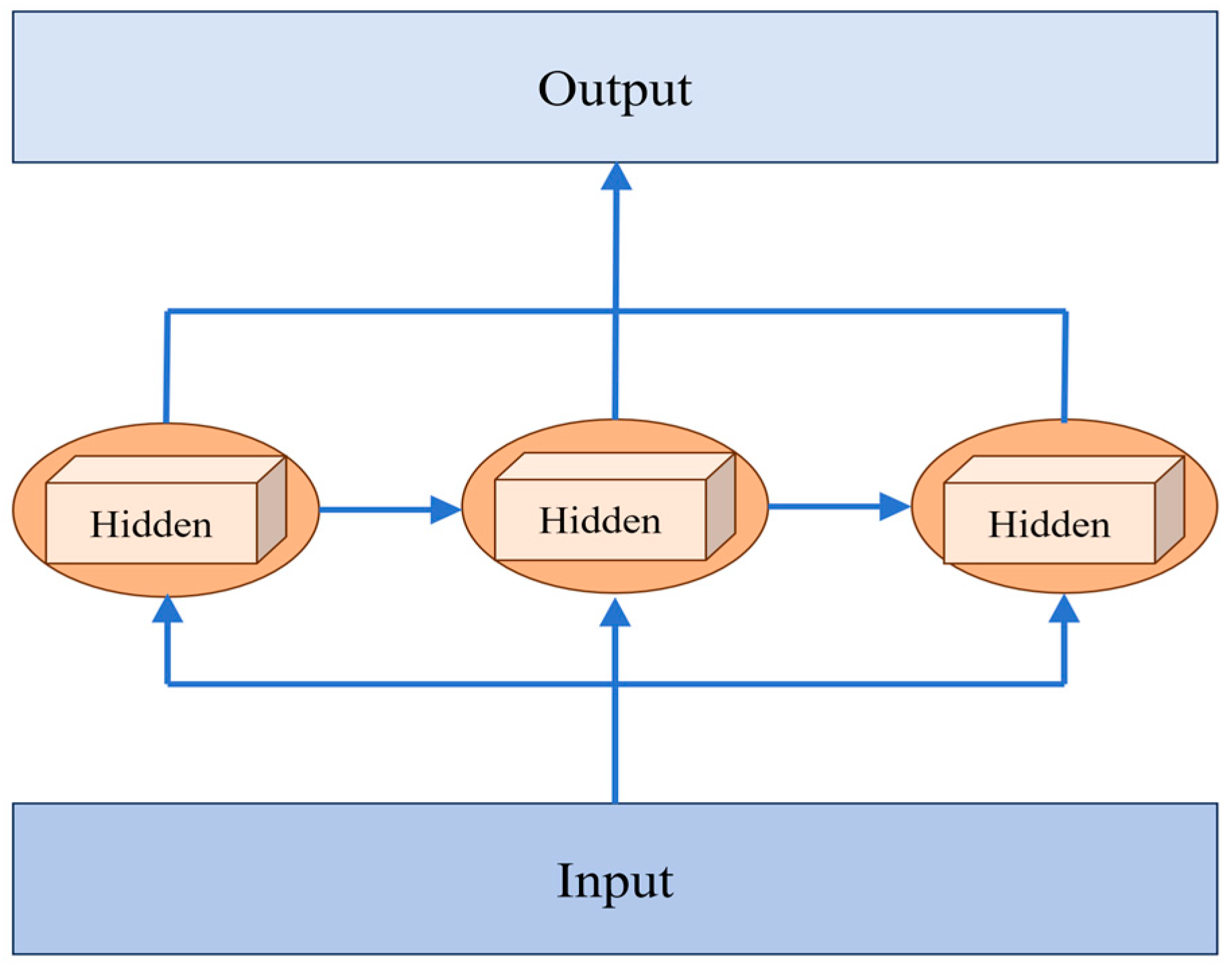
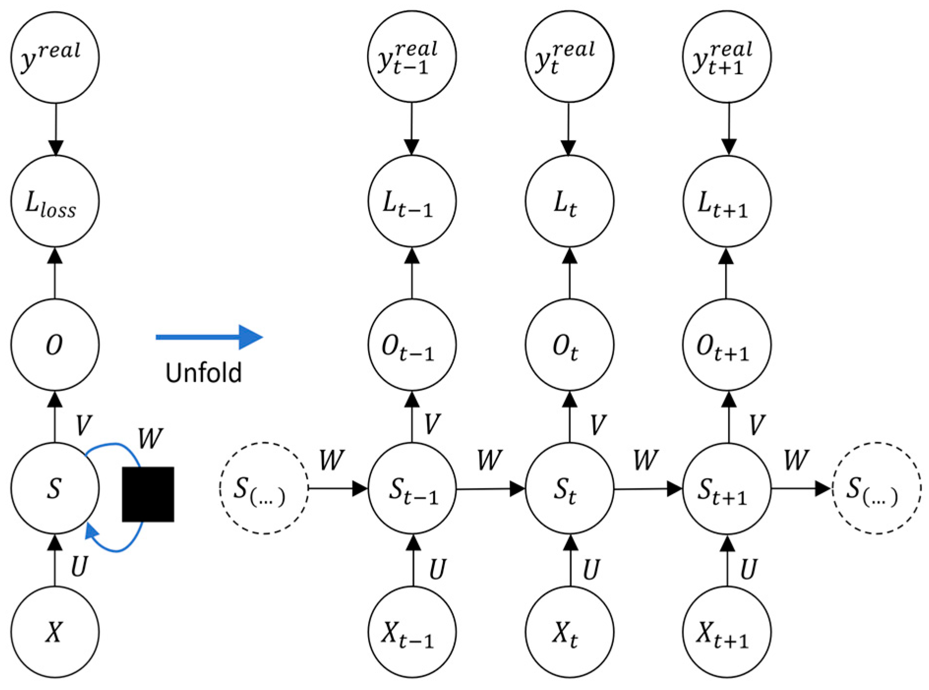
3.1. Architecture of RNN

RNN is a cyclic structure with excellent learning capabilities [31]. The structure of the RNN model is shown in Figure 2. RNN consists of three components: the input layer, hidden layer, and output layer. Figure 3 shows a schematic of the cyclic and unfolded structures of an RNN: X is the input; U is the weight matrix from the input layer to the hidden layer; S is the hidden state; V is the weight matrix from the hidden layer to the output layer; W is the weight matrix from hidden state to hidden state; O is the output; L l o s s is the loss function; and y r e a l is the real value of data.
Unlike DNN and CNN, RNN not only considers the input at the current time step but also considers the hidden state from the previous time step. In traditional neural network models, data flow sequentially from the input layer to the hidden layer and then to the output layer, with no connections between nodes within the same layer. Such structure limits the ability of DNN and CNN to process sequential data effectively. In contrast, the nodes within each layer are interconnected in an RNN, and each hidden layer node passes information to the corresponding node in the same hidden layer in the next time step. This structure enables an RNN to capture temporal dependencies in sequential data.
The forward propagation process of an RNN can be seen as calculating the input of each time step in a sequence while passing the hidden state of the previous time step as input to the current time step. Therefore, the current output can be influenced by memorizing the previous information. At each time step, the current input and the state of the previous time step are weighted and summed, and a non-linear transformation is performed through an activation function. The activation function can help the network capture information from the previous time step and pass it to the current time step, thereby helping the network remember the previous state to generate the output for the current time step and a new hidden state for subsequent computations.
The forward propagation formulas of an RNN are as follows [36], with the grid structure for forward propagation shown in Figure 4:
S t = tanh W X X t + W S S t 1 + b t 1 * ,
y ^ t = s o f t m a x W V S t + b t 2 * ,
where X t , S t , and y ^ t represent the input, the hidden state that contains recurrent information from the previous time step, and the output at the time step t . W X represents the weight matrix from input to hidden state, W S represents the weight matrix from hidden state to hidden state, W V represents the weight matrix from hidden state to output layer, b t 1 * is the bias of the hidden state, b t 2 * is the bias of the output layer, and s o f t m a x is the normalized exponential function.
To optimize the parameters of an RNN data-driven model, backpropagation through time (BPTT) is applied to update the model parameters using gradient descent based on the difference between the model output and the real label. The gradient descents [43] of the loss function L l o s s t related to W S , W X , and W V are given as follows:
L l o s s t W S = L l o s s t W S t + + L l o s s t W S 3 + L l o s s t W S 2 + L l o s s t W S 1 = L l o s s t O t O t S t S t W S t + k = 1 t 1 L l o s s t O t O t S t j = k + 1 t S j S j 1 S k W S ( k ) ,
L l o s s t W X = L l o s s t W X t + + L l o s s t W X 3 + L l o s s t W X 2 + L l o s s t W X 1 = L l o s s t O t O t S t S t W X t + k = 1 t 1 L l o s s t O t O t S t j = k + 1 t S j S j 1 S k W X ( k ) ,
L l o s s W V = t = 1 n L l o s s t O t O t S t S t W V ,
where S j S j 1 = t a n h W X X t + W s S t 1 + b t 1 * W s . W S t represents the weight matrix from hidden state to hidden state at the t t h time step, W X t represents the weight matrix from input to hidden state at the t t h time step, and W V t represents the weight matrix from hidden state to output layer at the t t h time step.
(a) Data preparation
The data used for time series prediction consists of displacement and velocity data of the vibration at the specified point on the studied laminated composite cantilever beam. To address varying feature scales in the raw data, the raw data are normalized using MinMaxScaler to scale all feature values into the range [ 0 ,   1 ] . A sliding window approach is employed to format the data for supervised learning, using the previous 10 time steps of displacement and velocity as input and the following time step as the prediction target.
The data are transformed into a 3D array with dimensions (samples, time steps, features) to meet the input requirements of RNN. The data are then split into training and testing datasets, which account for 60% and 40% of the normalized temporal sequences, respectively. The training set is used to train the RNN model, while the testing set is used to evaluate the RNN model’s prediction performance and generalization ability. During model training, the test set is also used to monitor the loss as validation data, but it is not involved in parameter updates. The strict time-based split ensures that the RNN model learns only from past data, thereby preventing overfitting and information leakage issues that may arise when the temporal order is disregarded.
(b) Architectures and hyperparameters
The RNN model architecture consists of an RNN layer with 50 hidden neurons, followed by a fully connected output layer. The RNN layer utilizes the ReLU activation function, and the network is compiled using the Adam optimizer and mean absolute error (MAE) as the loss function. The model is trained for 1000 epochs with a batch size of 128, and the total training time for 1000 epochs was approximately 300 s.
(c) Model verification
The trained model is evaluated based on the testing data. Predictions are performed and then inverse-transformed to restore the original data scale. Performance is assessed using root mean square error (RMSE) and MAE, which provide quantitative measures of the model’s predictive accuracy.

3.2. Loss Function

RMSE and MAE are employed as loss functions to evaluate the discrepancy between the data-driven model’s predictions and the original chaotic vibration time-series data. Based on RMSE and MAE, both the training and generalization performance of RNN are evaluated, respectively, as follows:
R M S E = 1 m i = 1 m y i p r e d y i r e a l 2 ,
M A E = 1 m i = 1 m y i p r e d y i r e a l ,
where y i r e a l and y i p r e d denote the real value and the predicted value at the i t h time step, and m is the length of the prediction sequence.
A smaller RMSE value indicates a smaller discrepancy between the RNN model’s predicted values and the real values, signifying better training performance and a higher degree of fit. Similarly, a smaller MAE value indicates higher stability of the RNN data-driven model.

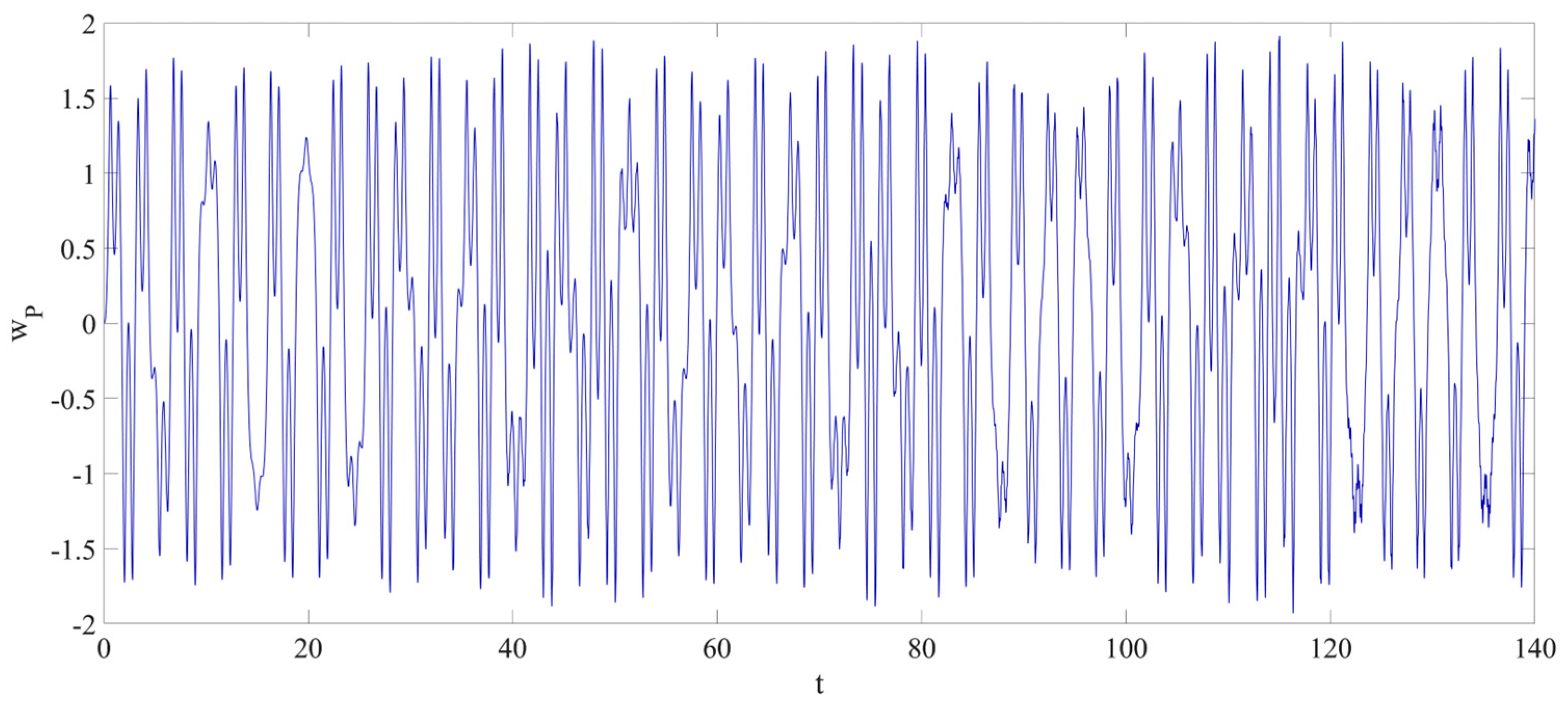
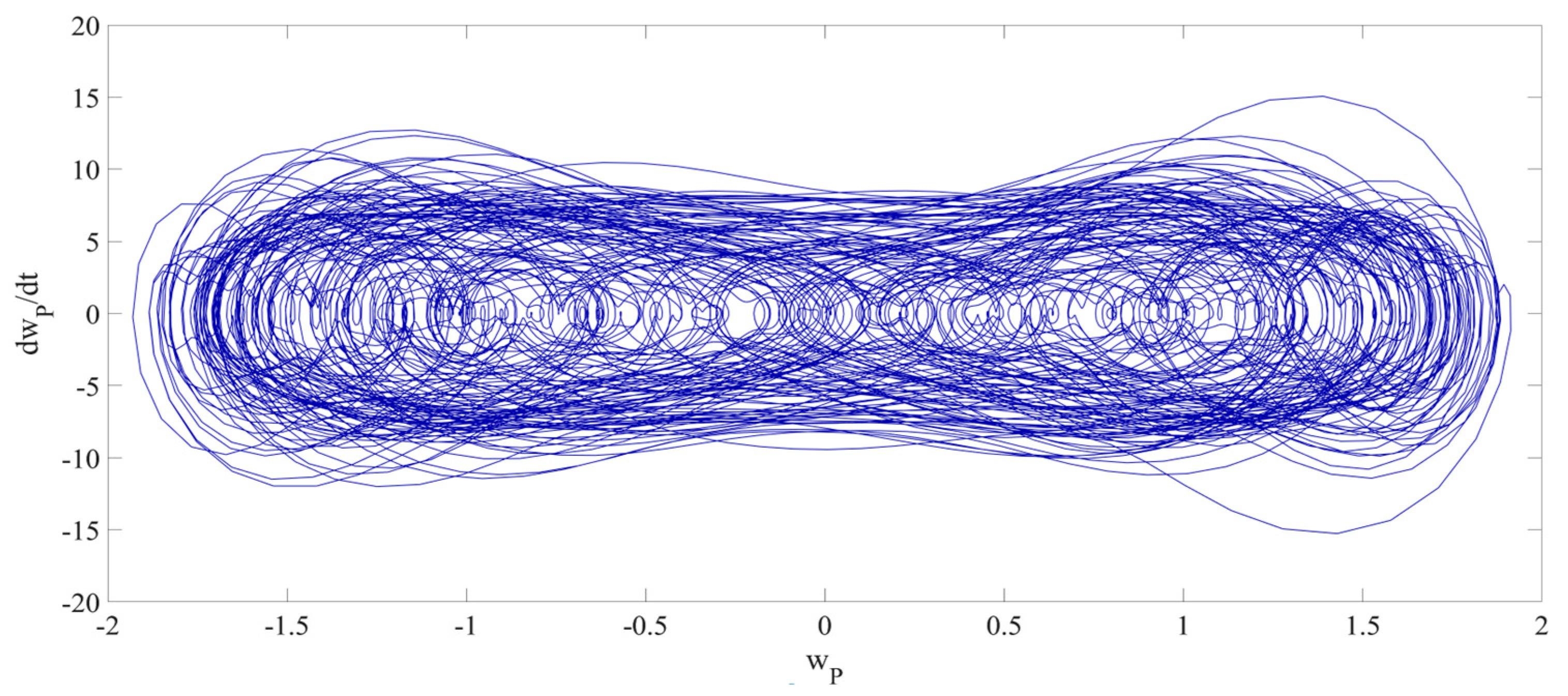
4. Numerical Simulation

In this section, the chaotic vibrations at x P = 0.75 are discovered and then predicted with the RNN data-driven model established in Equations (19)–(25).
Numerical simulations of the nonlinear dynamic responses are performed using a fourth-order Runge–Kutta method and implemented in MATLAB R2022b. The time step is fixed at 0.01 non-dimensional time units, and the total simulation duration is 140 non-dimensional time units. The simulated displacement and velocity response data are used to train and evaluate the accuracy of the RNN data-driven model. The RNN data-driven model is implemented using the Keras framework in Python.
The coefficients of the beam are as follows:
l = 0.5   m ,   b = 0.02   m ,   h = 0.01   m .

4.1. Predictions Corresponding to Different Q 1

The numerical simulations in this section are performed based on the following initial conditions:
w 1,1 0 = 0 ,   w 1,2 0 = 0 ,   w 2,1 0 = 0 ,   w 2,2 0 = 0 .
With Q 2 = 20 π , chaotic vibrations were observed for two different values of Q 1 and then predicted with the previously established RNN data-driven model.
(a) Q 1 = 5450   P a
When Q 1 = 5450   P a , the chaotic vibration of the laminated composite cantilever beam is shown in Figure 5, corresponding to a dimensionless time interval of t 0,140 . During this time interval, the chaotic vibration features a maximum amplitude close to 2.0, as shown in Figure 5. The 2D phase diagram and the first two vibration modes are provided in Figure 6 and Figure 7, respectively.
Figure 8 presents the predicted displacement and velocity time series curves for t 126 , 140 . The blue solid line represents the real displacement and velocity values obtained from numerical simulations, while the red dashed line represents the predicted values derived from the RNN data-driven model. A comparison of the results reveals a strong agreement between the real and predicted data, demonstrating the high accuracy of the RNN data-driven model in capturing both the maximum and minimum values of the chaotic vibration amplitude. This level of precision enables more reliable predictions of chaotic vibrations in subsequent time steps. To further illustrate the comparison, Figure 9 and Figure 10 present the 2D and 3D phase diagram comparisons, respectively, highlighting the close alignment between the real and predicted trajectories.
(b) Q 1 = 3450   P a
When Q 1 = 3450   P a , Figure 11 depicts the chaotic vibration of the laminated composite cantilever beam over a dimensionless time interval t 0 , 140 . As shown in Figure 11, the chaotic vibration is observed, and the maximum amplitude of the cantilever beam approaches 2.0. Moreover, Figure 12 and Figure 13 show the 2D phase diagram along with the first-order and second-order vibrations, providing a thorough representation of the chaotic vibration.
In Figure 14a,b, the two curves align closely, indicating the high accuracy of the RNN data-driven model in predicting chaotic vibrations in the studied cantilever structure. The model effectively captures the displacement and velocity data of the identified chaotic vibration, with minimal error between the real and predicted values. Figure 15 and Figure 16 present the 2D and 3D phase diagrams of the prediction results, respectively, where the real and predicted values exhibit a high degree of agreement.

4.2. Prediction Corresponding to Different Q 2

The numerical simulations in this section are performed based on Equation (27). With Q 1 = 4500   P a , chaotic vibrations were identified for different values of Q 2 and then predicted with the previously established RNN data-driven model.
(a) Q 2 = 23.0 π
When Q 2 = 23.0 π , the vibration of the laminated composite cantilever beam is shown in Figure 17, over a dimensionless time interval t 0 , 140 . During this time interval, a chaotic vibration is observed in Figure 17, and the maximum amplitude of the cantilever beam is close to 2.0. Figure 18 and Figure 19 present the 2D phase diagram, and the responses of the first two vibration modes, providing a detailed illustration of the chaotic vibration.
Figure 20 shows a comparison between the real value and predicted value of displacement and velocity, revealing a high degree of consistency between the two. Figure 21 and Figure 22 present the error between the real data and predicted results for the 2D and 3D phase diagrams, demonstrating the capability of RNN in accurately predicting chaotic vibrations.
(b) Q 2 = 41.0 π
When Q 2 = 41.0 π , the vibration of the laminated composite cantilever beam is illustrated in Figure 23, over a dimensionless time interval t 0 , 140 . A chaotic vibration is observed in Figure 23 within the time interval t 0 , 140 , and the maximum amplitude of the cantilever beam is close to 2.1. Figure 24 and Figure 25 present the 2D phase diagram and the first two vibration modes, providing a detailed depiction of the chaotic vibration.
Figure 26 shows a comparison between the real value and the predicted value of the response of the laminated composite beam, revealing a high degree of consistency between the two. In addition, both a 2D phase diagram provided in Figure 27 and a 3D phase diagram provided in Figure 28 are presented to compare the predicted results with the real data. The results show that RNN can accurately predict the chaotic vibration of the laminated composite cantilever beam.

4.3. Prediction Corresponding to Different Initial Conditions

Chaotic systems are known for their extreme sensitivity to initial conditions. Small disturbances in the initial state may lead to completely different trajectories. It is crucial to test the robustness and generalization ability of RNN for predicting chaotic vibrations under changes in initial conditions. Therefore, in this section, the predictive ability of the RNN model for chaotic vibrations is further validated by changing the initial conditions.
With Q 1 = 4500   P a and Q 2 = 41 π , chaotic vibrations were identified, and the previously trained RNN model was used to predict the system responses under different initial conditions by individually changing one component of the initial conditions, where the initial conditions were w 1,1 0 = 0 , w 1,2 0 = 0 , w 2,1 0 = 0 , and w 2,2 0 = 0 .
(a) w 1,1 0 = 0.001 , w 1,2 0 = 0 , w 2,1 0 = 0 , w 2,2 0 = 0
When w 1,1 0 = 0.001 , the vibration of the laminated composite cantilever beam is shown in Figure 29. Chaotic vibration is observed within the time interval t 0,140 , and the maximum displacement amplitude reaches approximately 2.0 . Figure 30 and Figure 31 present the 2D phase diagram and the first two modal responses, respectively, providing a detailed illustration of the chaotic vibration.
Figure 32 illustrates the comparison between the real value and predicted value of the displacement and velocity. A high level of agreement can be observed between the two curves. In addition, Figure 33 and Figure 34 present the 2D and 3D phase diagrams of the chaotic vibration, respectively. The results indicate that the RNN model can accurately predict the chaotic vibration of the laminated composite cantilever beam, even in the presence of initial condition perturbations.
(b) w 1,1 0 = 0 , w 1,2 0 = 0.001 , w 2,1 0 = 0 , w 2,2 0 = 0
When w 1,2 0 = 0.001 , the vibration of the laminated composite cantilever beam is shown in Figure 35. Within the time interval t 0 , 140 , the laminated composite cantilever beam exhibits chaotic vibration, with a maximum amplitude of approximately 2.1 . Figure 36 and Figure 37 display the 2D phase diagram and the first two vibration modes, providing a detailed characterization of the chaotic vibration.
Figure 38 presents the comparison between the real and predicted displacement and velocity responses of the laminated composite cantilever beam. As shown in Figure 38, the two curves remain highly consistent. Figure 39 and Figure 40 display the 2D and 3D phase diagrams, providing comparative views of the real value and predicted value from different spatial perspectives. These results confirm that the RNN model is capable of accurately predicting the chaotic vibration of the laminated composite cantilever beam.
(c) w 1,1 0 = 0 , w 1,2 0 = 0 , w 2,1 0 = 0.001 , w 2,2 0 = 0
When w 2,1 0 = 0.001 , the chaotic vibration of the laminated composite cantilever beam is shown in Figure 41. Within the time interval t 0 ,   140 , the maximum amplitude reaches approximately 2.1 . Figure 42 and Figure 43 present the 2D phase diagram and the first two vibration modes of the chaotic vibration, respectively.
Figure 44 illustrates the comparison between the real and predicted displacement and velocity responses. As observed in Figure 44, the predicted curves closely match the real curves. In addition, both a 2D phase diagram provided in Figure 45 and a 3D phase diagram provided in Figure 46 are presented to compare the predicted results with the real data. The results show that the RNN model can accurately predict the chaotic vibration of the laminated composite cantilever beam even under perturbed initial conditions.
(d) w 1,1 0 = 0 , w 1,2 0 = 0 , w 2,1 0 = 0 , w 2,2 0 = 0.001
When w 2,2 0 = 0.001 , the laminated composite cantilever beam exhibits chaotic vibration, as shown in Figure 47. Within the dimensionless time interval t 0 ,   140 , the maximum amplitude reaches approximately 2.0 . Figure 48 and Figure 49 display the 2D phase diagram and the first two vibration modes of the chaotic vibration, respectively, providing a more detailed illustration of the chaotic vibration of the laminated composite cantilever beam.
Figure 50 presents the comparison between the real and predicted displacement and velocity responses. A comparison of the results reveals a strong agreement between the real and predicted data, demonstrating the high accuracy of the RNN model in capturing both the maximum and minimum values of the chaotic vibration amplitude. Figure 51 and Figure 52 illustrate the comparisons in the 2D and 3D phase diagrams, indicating that the RNN model demonstrates high accuracy in capturing the chaotic vibration of the laminated composite cantilever beam and is capable of reliably predicting its dynamic behavior under chaotic conditions.
Table 1 presents a brief summary of the prediction errors of the RNN data-driven model for the above four chaotic vibrations in terms of displacement and velocity. By examining the data in Table 1, it can be observed that the RNN data-driven model consistently achieves small MAE and RMSE values for both displacement and velocity. Hence, these results indicate that RNN demonstrates strong prediction performance for displacement and velocity in chaotic vibrations of a laminated composite beam.
Table 2 summarizes the prediction performance of the RNN model under different initial conditions, with the external excitation given as 4500   P a   s i n 41 π t . In each case, only one component of the initial state is varied, while the others are set to 0 . As shown in Table 2, the RNN model maintains low prediction errors across all conditions, with MAE ranging from 0.013 to 0.022 and RMSE ranging from 0.021 to 0.038 . These results further demonstrate the robustness and accuracy of the RNN model in predicting the chaotic vibration of the laminated composite cantilever beam.
The RNN model does not rely on explicit physical governing equations. Its high accuracy in predicting the chaotic vibrations of the laminated composite cantilever beam indicates that it can effectively capture the intrinsic nonlinear dynamic characteristics of the system. During training, the RNN model receives sequences of displacement and velocity over the previous 10 time steps. This multivariate time-series input contains key informational features of chaotic systems, such as amplitude modulation, phase variation, and nonlinear coupling between state variables. The recurrent structure of the RNN allows it to update its internal state at each time step and gradually accumulate the system’s evolution history. The state memory mechanism enables the RNN model to learn the temporal dependencies between input variables. The high consistency between the predicted results and the phase diagrams implicitly verifies the effectiveness of the RNN model in learning the dynamic behavior of chaotic systems.

5. Conclusions

The RNN data-driven model has been demonstrated to accurately and robustly predict chaotic vibrations in the laminated composite cantilever beam under various perturbed initial conditions. Unlike conventional numerical simulation methods that rely on explicit governing equations and domain expertise, the RNN model learns the dynamic behavior implicitly from historical time-series data. The results demonstrate that the RNN model can accurately predict the chaotic vibrations of the laminated composite cantilever beam, providing a valuable complement to traditional simulation techniques in the context of chaos and structural dynamics.
This study focuses on the prediction of chaotic vibrations in a multi-dimensional nonlinear dynamic system of the laminated composite cantilever beam. Based on the numerical simulation results, the main conclusions and contributions are summarized as follows:
1. The RNN data-driven model is capable of automatically learning the time-series characteristics of chaotic vibrations from data generated by numerical simulation and accurately predicting the nonlinear vibrations of the laminated composite cantilever beam.
2. The model’s predictive performance was evaluated under various combinations of excitation magnitudes and angular frequencies. The results showed that the maximum MAE and RMSE reached 0.041 and 0.067 , respectively, indicating that the RNN model exhibits good prediction accuracy and numerical stability in capturing chaotic vibrations.
3. Given the strong sensitivity of chaotic systems to initial conditions, the robustness of the RNN model was further tested by introducing multiple perturbed initial states. The results demonstrated that the RNN model maintained reliable performance even under disturbed initial conditions, with a maximum MAE of 0.022 and RMSE of 0.038 , confirming its robustness and resistance to initial conditions.
Therefore, the predictive analysis demonstrates that the RNN data-driven model is a powerful algorithm for predicting the chaotic vibrations of the widely applied laminated composite cantilever beam structures.

6. Future Development

This study has demonstrated the effectiveness of the RNN model in predicting chaotic vibrations of the laminated composite cantilever beam. Nevertheless, several promising directions remain for further investigation, including the following:
Firstly, future research should focus on extending the RNN model to more complex structural problems involving material nonlinearity, boundary nonlinearity, and other types of nonlinear behavior, in order to assess its applicability and generalization capability across a broader range of nonlinear dynamic systems.
Secondly, constructing confidence intervals or prediction intervals will allow for a more comprehensive evaluation of both the RNN model’s response to input uncertainty and its overall robustness.
Thirdly, by introducing interpretability techniques such as attention mechanisms and feature attribution, future studies can analyze the temporal features learned during training and gain deeper insight into their physical significance, thereby enhancing the transparency and interpretability of the RNN model.

Author Contributions

X.L. (Xudong Li): methodology, investigation, writing—original draft. L.S.: investigation, data curation, resources, funding acquisition, supervision. X.L. (Xiaopei Liu): conceptualization, methodology, writing—review and editing, supervision. Y.D.: resources, funding acquisition, supervision. All authors have read and agreed to the published version of the manuscript.

Funding

This research was funded by the National Natural Science Foundation of China (NNSFC) through the grant No. 11602234, the talent scientific research fund of Liaoning Petrochemical University (No. 2017XJJ-058), and Liaoning Provincial Education Department Basic Scientific Research Project for Youth (No. LJ212410148060).

Institutional Review Board Statement

Not applicable.

Informed Consent Statement

Not applicable.

Data Availability Statement

The original contributions presented in this study are included in the article. Further inquiries can be directed to the corresponding author(s).

Conflicts of Interest

The authors declare that they have no known competing financial interests or personal relationships that could have influenced the work reported in this paper.

Appendix A

A 11 2 u 0 x 2 + A 11 w 0 x 2 w 0 x 2 I 0 d 2 u 0 d t 2 = 0 ,
A 55 + 6 D 55 c 1 9 F 55 c 1 2 x + D 11 2 F 11 c 1 + H 11 c 1 2 2 x x 2 + A 55 + 6 D 55 c 1 9 F 55 c 1 2 w 0 x + F 11 c 1 + H 11 c 1 2 3 w 0 x 3 K 2 d 2 x d t 2 + c 1 J 4 x d 2 w 0 d t 2 = 0 ,
A 11 w 0 x 2 u 0 x 2 + A 11 u 0 x 2 w 0 x 2 + 3 2 A 11 w 0 x 2 2 w 0 x 2 + c 1 F 11 c 1 H 11 3 x x 3 c 1 2 H 11 4 w 0 x 4 + A 55 6 c 1 D 55 + 9 c 1 2 F 55 x x + A 55 6 c 1 D 55 + 9 c 1 2 F 55 2 w 0 x 2 I 0 d 2 w 0 d t 2 + c 1 2 I 6 2 x 2 d 2 w 0 d t 2 c 1 J 4 x d 2 x d t 2 + q c d w 0 d t = 0 ,
where A 11 , D 11 , F 11 , H 11 , A 55 , D 55 , F 55 , I 0 , I 4 , I 6 , J 4 , and K 2 , are given below,
A 11 , D 11 , F 11 , H 11 = k = 1 3 z k z k + 1 Q 11 k 1 , z 2 , z 4 , z 6 d z ,
A 55 , D 55 , F 55 = k = 1 3 z k z k + 1 Q 13 k 1 , z 2 , z 4 d z ,
I 0 , I 4 , I 6 , = k = 1 3 z k z k + 1 ρ k 1 , z 4 , z 6 d z ,
J 4 = I 4 I 6 c 1 ,
K 2 = ( I 2 2 I 4 c 1 + I 6 c 1 2 ) ,
and k = 1 , 2 , 3 represents the layer index. In addition, Q i j ( 1 ) , Q i j ( 2 ) and Q i j ( 3 ) are the elastic parameters for the lower layer, middle layer, and upper layer respectively, and ρ ( 1 ) , ρ ( 2 ) and ρ ( 3 ) are the densities respectively.
I = Ω z 2 d A z y = b h 3 12 ,   I 0 = k = 1 3 z k 1 z k ρ ( k ) d z .
A = I 0 ρ h ,   B = 1 l 2 c 1 I 4 ρ h ,   C = 1 l 4 c 1 J 4 ρ h F 11 c 1 D 11 A 55 6 D 55 c 1 + 9 F 55 c 1 2 ,   D = c ρ h τ ,   F = h A 11 2 ρ τ 2 l 4 ,   G = D 11 ρ h τ 2 l 4 , H = c 1 F 11 c 1 H 11 ρ h τ 2 l 6 F 11 c 1 D 11 A 55 6 D 55 c 1 + 9 F 55 c 1 2 ;
w ˙ 1,1 = w 1,2 w ˙ 1,2 = T 11 w 1,2 + T 12 w 1,1 + T 13 w 2,2 + T 14 w 2,1 + T 15 w 1,1 3 + T 16 w 1,1 2 w 2,1 + T 17 w 2,1 2 w 1,1 + T 18 w 2,1 3 + T 19 q w ˙ 2,1 = w 2,2 w ˙ 2,2 = T 21 w 1,2 + T 22 w 1,1 + T 23 w 2,2 + T 24 w 2,1 + T 25 w 1,1 3 + T 26 w 1,1 2 w 2,1 + T 27 w 2,1 2 w 1,1 + T 28 w 2,1 3 + T 29 q ,
where T 1 i and T 2 i   i = 1 , 2 , , 9 are given below,
T 11 = U 1 S 1 b + U 2 S 2 b ,   T 12 = U 1 S 1 c + U 2 S 2 c ,   T 13 = U 1 S 1 e + U 2 S 2 e , T 14 = U 1 S 1 f + U 2 S 2 f ,   T 15 = U 1 S 1 g + U 2 S 2 g ,   T 16 = U 1 S 1 h + U 2 S 2 h , T 17 = U 1 S 1 i + U 2 S 2 i ,   T 18 = U 1 S 1 j + U 2 S 2 j ,   T 19 = U 1 S 1 k + U 2 S 2 k ;
T 21 = U 3 S 1 b + U 4 S 2 b ,   T 22 = U 3 S 1 c + U 4 S 2 c ,   T 23 = U 3 S 1 e + U 4 S 2 e , T 24 = U 3 S 1 f + U 4 S 2 f ,   T 25 = U 3 S 1 g + U 4 S 2 g ,   T 26 = U 3 S 1 h + U 4 S 2 h , T 27 = U 3 S 1 i + U 4 S 2 i ,   T 28 = U 3 S 1 j + U 4 S 2 j ,   T 29 = U 3 S 1 k + U 4 S 2 k ;
U 1 = S 2 d S 1 a S 2 d S 1 d S 2 a ,   U 2 = S 1 d S 1 a S 2 d S 1 d S 2 a ,   U 3 = S 2 a S 1 a S 2 d S 1 d S 2 a , U 4 = S 1 a S 1 a S 2 d S 1 d S 2 a ;
S 1 a = 1.000000000 A + 0.8581959666 B 12.35961914 C , S 1 b = 1.000000000 D , S 1 c = + 2.005226046 E 12.35961914 G + 10.60697530 H , S 1 d = 11.74232364 B , S 1 e = 0.0000000000 , S 1 f = 6.312477510 E 5700.676306 H , S 1 g = + 3.994625840 F , S 1 h = 67.36709586 F , S 1 i = + 201.8072370 F , S 1 j = 381.7008418 F , S 1 k = + 0.7829242108 ; S 2 a = + 1.873752475 B , S 2 b = 0.0000000000 , S 2 c = + 0.5091766256 E + 23.15886696 H , S 2 d = 1.000000000 A 13.29402727 B 485.4811154 C , S 2 e = 1.000000000 D , S 2 f = + 2.018651170 E 485.4811154 G 6453.999206 H , S 2 g = + 8.721714324 F , S 2 h = 89.63073490 F , S 2 i = + 257.8009342 F , S 2 j = 432.1411636 F , S 2 k = + 0.4339831449

References

  1. Jin, F.; Zhao, C.; Xu, P.; Xue, J.; Xia, F. Nonlinear eccentric bending and buckling of laminated cantilever beams actuated by embedded pre-stretched SMA wires. Compos. Struct. 2022, 284, 115211. [Google Scholar] [CrossRef]
  2. Zhang, W.; Sun, L.; Yang, X.D.; Jia, P. Nonlinear dynamic behaviors of a deploying-and-retreating wing with varying velocity. J. Sound Vib. 2013, 332, 6785–6797. [Google Scholar] [CrossRef]
  3. Wang, R.; Yao, D.; Zhang, J.; Xiao, X.; Jin, X. Sound-insulation prediction model and multi-parameter optimisation design of the composite floor of a high-speed train based on machine learning. Mech. Syst. Signal Process. 2023, 200, 110631. [Google Scholar] [CrossRef]
  4. Kormanikova, E.; Kotrasova, K.; Melcer, J.; Valaskova, V. Numerical investigation of the dynamic responses of fibre-reinforced polymer composite bridge beam subjected to moving vehicle. Polymers 2022, 14, 812. [Google Scholar] [CrossRef]
  5. He, C.; Kong, Q.; Ji, K.; Xiong, Q.; Yuan, C. Deep learning-based analysis of interface performance between brittle engineering materials and composites. Expert Syst. Appl. 2024, 255, 124920. [Google Scholar] [CrossRef]
  6. Krishnamurthy, V. Predictability of weather and climate. Earth Space Sci. 2019, 6, 1043–1056. [Google Scholar] [CrossRef]
  7. Bihlo, A. A generative adversarial network approach to (ensemble) weather prediction. Neural Netw. 2021, 139, 1–16. [Google Scholar] [CrossRef]
  8. Zhang, W.; Wang, F.; Yao, M. Global bifurcations and chaotic dynamics in nonlinear nonplanar oscillations of a parametrically excited cantilever beam. Nonlinear Dyn. 2005, 40, 251–279. [Google Scholar] [CrossRef]
  9. Bouadjadja, S.; Tati, A.; Guerira, B. Analytical and experimental investigations on large deflection analysis of composite cantilever beams. Mech. Adv. Mater. Struct. 2020, 29, 118–126. [Google Scholar] [CrossRef]
  10. Cheng, Q.; Wang, Q.M.; Lv, Z. Theoretical and experiment optimization research of a frequency up-converted piezoelectric energy harvester based on impact and magnetic force. Eng. Res. Express 2024, 6, 035314. [Google Scholar] [CrossRef]
  11. Wu, H.; Kitipornchai, S.; Yang, J. Thermal buckling and postbuckling of functionally graded graphene nanocomposite plates. Mater. Des. 2017, 132, 430–441. [Google Scholar] [CrossRef]
  12. Guo, X.; Zhang, B.; Cao, D.; Sun, L. Influence of nonlinear terms on dynamical behavior of graphene reinforced laminated composite plates. Appl. Math. Model. 2020, 78, 169–184. [Google Scholar] [CrossRef]
  13. Van Viet, N.; Zaki, W.; Umer, R. Bending theory for laminated composite cantilever beams with multiple embedded shape memory alloy layers. J. Intell. Mater. Syst. Struct. 2019, 30, 1549–1568. [Google Scholar] [CrossRef]
  14. Jun, L.; Xiaobin, L.; Hongxing, H. Free vibration analysis of third-order shear deformable composite beams using dynamic stiffness method. Arch. Appl. Mech. 2009, 79, 1083–1098. [Google Scholar] [CrossRef]
  15. Amabili, M.; Ferrari, G.; Ghayesh, M.H.; Hameury, C.; Zamal, H.H. Nonlinear vibrations and viscoelasticity of a self-healing composite cantilever beam: Theory and experiments. Compos. Struct. 2022, 294, 115741. [Google Scholar] [CrossRef]
  16. Zhang, W.; Zhao, M.H.; Guo, X.Y. Nonlinear responses of a symmetric cross-ply composite laminated cantilever rectangular plate under in-plane and moment excitations. Compos. Struct. 2013, 100, 554–565. [Google Scholar] [CrossRef]
  17. Liu, X.; Sun, L. Chaotic vibration control of a composite cantilever beam. Sci. Rep. 2023, 13, 17946. [Google Scholar] [CrossRef]
  18. Guo, X.; Jiang, P.; Cao, D. Influence of piezoelectric performance on nonlinear dynamic characteristics of MFC shells. Complexity 2019, 2019, 1970248. [Google Scholar] [CrossRef]
  19. Zhang, W.; Ren, L.L.; Zhang, Y.F.; Guo, X.T. Chaotic snap-through vibrations of bistable asymmetric deployable composite laminated cantilever shell under foundation excitation and application to morphing wing. Compos. Struct. 2024, 343, 118261. [Google Scholar] [CrossRef]
  20. Sun, L.; Li, X.D.; Liu, X. Control of large amplitude limit cycle of a multi-dimensional nonlinear dynamic system of a composite cantilever beam. Sci. Rep. 2024, 14, 10771. [Google Scholar] [CrossRef]
  21. Ghazoul, T.; Benatta, M.A.; Khatir, A.; Beldjelili, Y.; Krour, B.; Bouiadjra, M.B. Analytical investigation on the buckling and free vibration of porous laminated FG-CNTRC plates. Vojnoteh. Glas. 2024, 72, 1242–1271. [Google Scholar] [CrossRef]
  22. Rosso, M.; Cuccurullo, S.; Perli, F.P.; Maspero, F.; Corigliano, A.; Ardito, R. A method to enhance the nonlinear magnetic plucking for vibration energy harvesters. Meccanica 2024, 59, 1577–1592. [Google Scholar] [CrossRef]
  23. Hao, Y.X.; Sun, K.C.; Li, H. Nonlinear dynamics of the GPR porous cantilever twisted plate near veering regions. Mech. Based Des. Struct. Mach. 2025, 1–27. [Google Scholar] [CrossRef]
  24. Qi, C.; Gao, F.; Li, H.-X.; Zhao, X.; Deng, L. A neural network-based distributed parameter model identification approach for microcantilever. Proc. Inst. Mech. Eng. Part C 2015, 230, 3663–3676. [Google Scholar] [CrossRef]
  25. Subramanian, A.; Mahadevan, S. Bayesian estimation of discrepancy in dynamics model prediction. Mech. Syst. Signal Process. 2019, 123, 351–368. [Google Scholar] [CrossRef]
  26. Teng, Q.; Zhang, L. Data driven nonlinear dynamical systems identification using multi-step CLDNN. AIP Adv. 2019, 9, 085311. [Google Scholar] [CrossRef]
  27. Cestnik, R.; Abel, M. Inferring the dynamics of oscillatory systems using recurrent neural networks. Chaos 2019, 29, 063128. [Google Scholar] [CrossRef]
  28. Huang, B.; Zheng, H.; Guo, X.; Yang, Y.; Liu, X. A Novel Model Based on DA-RNN Network and Skip Gated Recurrent Neural Network for Periodic Time Series Forecasting. Sustainability 2022, 14, 326. [Google Scholar] [CrossRef]
  29. Uribarri, G.; Mindlin, G.B. Dynamical time series embeddings in recurrent neural networks. Chaos Solitons Fractals 2022, 154, 111612. [Google Scholar] [CrossRef]
  30. Dudukcu, H.V.; Taskiran, M.; Cam Taskiran, Z.G.; Yildirim, T. Temporal convolutional networks with RNN approach for chaotic time series prediction. Appl. Soft Comput. 2023, 133, 109945. [Google Scholar] [CrossRef]
  31. Sangiorgio, M.; Dercole, F.; Guariso, G. Forecasting of noisy chaotic systems with deep neural networks. Chaos Solitons Fractals 2021, 153, 111570. [Google Scholar] [CrossRef]
  32. Sun, Y.; Zhang, L.; Yao, M. Chaotic time series prediction of nonlinear systems based on various neural network models. Chaos Solitons Fractals 2023, 175, 113971. [Google Scholar] [CrossRef]
  33. Zhang, X.; Zhong, C.; Zhang, J.; Wang, T.; Ng, W.W.Y. Robust recurrent neural networks for time series forecasting. Neurocomputing 2023, 526, 143–157. [Google Scholar] [CrossRef]
  34. Khatir, A.; Capozucca, R.; Khatir, S.; Magagnini, E.; Benaissa, B.; Thanh, C.L.; Wahab, M.A. A new hybrid PSO-YUKI for double cracks identification in CFRP cantilever beam. Compos. Struct. 2023, 311, 116803. [Google Scholar] [CrossRef]
  35. Khatir, A.; Capozucca, R.; Khatir, S.; Magagnini, E.; Benaissa, B.; Cuong-le, T. An efficient improved Gradient Boosting for strain prediction in Near-Surface Mounted fiber-reinforced polymer strengthened reinforced concrete beam. Front. Struct. Civ. Eng. 2024, 18, 1148–1168. [Google Scholar] [CrossRef]
  36. Wang, L.; Dai, L.; Sun, L. ConvLSTM-based spatiotemporal and temporal processing models for chaotic vibration prediction of a microbeam. Commun. Nonlinear Sci. Numer. Simul. 2025, 140, 108411. [Google Scholar] [CrossRef]
  37. Khatir, A.; Capozucca, R.; Khatir, S.; Magagnini, E.; Cuong-le, T. Enhancing damage detection using reptile search algorithm-optimized neural network and frequency response function. J. Vib. Eng. Technol. 2025, 13, 88. [Google Scholar] [CrossRef]
  38. Osmani, A.; Shamass, R.; Tsavdaridis, K.D.; Ferreira, F.P.V.; Khatir, A. Deflection predictions of tapered cellular steel beams using analytical models and an artificial neural network. Buildings 2025, 15, 992. [Google Scholar] [CrossRef]
  39. Reddy, J.N. Mechanics of Laminated Composite Plates and Shells: Theory and Analysis; Taylor & Francis: Oxfordshire, UK, 2003. [Google Scholar]
  40. Sun, L.; Hou, F.L.; Liu, X.P. Nonlinear vibration control of a high-dimensional nonlinear dynamic system of an axially-deploying elevator cable. Mathematics 2025, 13, 1289. [Google Scholar] [CrossRef]
  41. Zhang, W.; Yang, J.H.; Zhang, Y.F.; Yang, S.W. Nonlinear transverse vibrations of angle-ply laminated composite piezoelectric cantilever plate with four-modes subjected to in-plane and out-of-plane excitations. Eng. Struct. 2019, 198, 109501. [Google Scholar] [CrossRef]
  42. Guo, X.Y.; Zhang, Y.M.; Luo, Z.; Cao, D.X. Nonlinear dynamics analysis of a graphene laminated composite plate based on an extended Rayleigh–Ritz method. Thin-Walled Struct. 2023, 186, 110673. [Google Scholar] [CrossRef]
  43. Khennour, M.E.; Bouchachia, A.; Kherfi, M.L.; Bouanane, K. Randomising the Simple Recurrent Network: A lightweight, energy-efficient RNN model with application to forecasting problems. Neural Comput. Appl. 2023, 35, 19707–19718. [Google Scholar] [CrossRef]
Figure 1. The structure of a three-layered laminated composite cantilever beam.
Applsci 15 06403 g001
Figure 2. Structure of RNN.
Applsci 15 06403 g002
Figure 3. Schematic of cyclic and unfolded structures of RNN.
Applsci 15 06403 g003
Figure 4. Grid structure for forward propagation of RNN.
Applsci 15 06403 g004
Figure 5. The vibration of the cantilever beam at x P for Q 1 = 5450   P a .
Applsci 15 06403 g005
Figure 6. 2D phase diagram at x P for Q 1 = 5450   P a .
Applsci 15 06403 g006
Figure 7. The vibrations for the first mode vibration and the second mode vibration: (a) w 1,1 ; (b) w 2,1 .
Applsci 15 06403 g007aApplsci 15 06403 g007b
Figure 8. Testing result for Q 1 = 5450   P a : (a) displacement comparison; (b) velocity comparison.
Applsci 15 06403 g008
Figure 9. Testing result for 2D phase diagram, t 126 , 140
Applsci 15 06403 g009
Figure 10. Testing result for 3D phase diagram, t 126 , 140
Applsci 15 06403 g010
Figure 11. The vibration of the cantilever beam at x P for Q 1 = 3450   P a .
Applsci 15 06403 g011
Figure 12. 2D phase diagram at x P for Q 1 = 3450   P a .
Applsci 15 06403 g012
Figure 13. The vibrations for the first mode vibration and the second mode vibration: (a) w 1,1 (b) w 2,1 .
Applsci 15 06403 g013
Figure 14. Testing result for Q 1 = 3450   P a : (a) displacement comparison; (b) velocity comparison.
Applsci 15 06403 g014
Figure 15. Testing result for 2D phase diagram, t 126 , 140
Applsci 15 06403 g015
Figure 16. Testing result for 3D phase diagram, t 126 , 140
Applsci 15 06403 g016
Figure 17. The vibration of the cantilever beam at x P for Q 2 = 23.0 π .
Applsci 15 06403 g017
Figure 18. 2D phase diagram at x P for Q 2 = 23.0 π .
Applsci 15 06403 g018
Figure 19. The vibrations for the first mode vibration and the second mode vibration: (a) w 1,1 ; (b) w 2,1 .
Applsci 15 06403 g019
Figure 20. Testing result for Q 2 = 23.0 π : (a) displacement comparison; (b) velocity comparison.
Applsci 15 06403 g020aApplsci 15 06403 g020b
Figure 21. Testing result for 2D phase diagram, t 126 , 140
Applsci 15 06403 g021
Figure 22. Testing result for 3D phase diagram, t 126 , 140
Applsci 15 06403 g022
Figure 23. The vibration of the cantilever beam at x P for Q 2 = 41.0 π .
Applsci 15 06403 g023
Figure 24. 2D phase diagram at x P for Q 2 = 41.0 π .
Applsci 15 06403 g024
Figure 25. The vibrations for the first mode vibration and the second mode vibration: (a) w 1,1 ; (b) w 2,1 .
Applsci 15 06403 g025
Figure 26. Testing result for Q 2 = 41.0 π : (a) displacement comparison; (b) velocity comparison.
Applsci 15 06403 g026
Figure 27. Testing result for 2D phase diagram, t 126 , 140
Applsci 15 06403 g027
Figure 28. Testing result for 3D phase diagram, t 126 , 140
Applsci 15 06403 g028
Figure 29. The vibration of the cantilever beam at x P for w 1,1 0 = 0.01 .
Applsci 15 06403 g029
Figure 30. 2D phase diagram at x P for w 1,1 0 = 0.01 .
Applsci 15 06403 g030
Figure 31. The vibrations for the first mode vibration and the second mode vibration: (a) w 1,1 ; (b) w 2,1 .
Applsci 15 06403 g031
Figure 32. Testing result for w 1,1 0 = 0.001 : (a) displacement comparison; (b) velocity comparison.
Applsci 15 06403 g032
Figure 33. Testing result for 2D phase diagram, t 126 , 140
Applsci 15 06403 g033
Figure 34. Testing result for 3D phase diagram, t 126 , 140
Applsci 15 06403 g034
Figure 35. The vibration of the cantilever beam at x P for w 1,2 0 = 0.001 .
Applsci 15 06403 g035
Figure 36. 2D phase diagram at x P for w 1,2 0 = 0.001 .
Applsci 15 06403 g036
Figure 37. The vibrations for the first mode vibration and the second mode vibration: (a) w 1,1 ; (b) w 2,1 .
Applsci 15 06403 g037
Figure 38. Testing result for w 1,2 0 = 0.001 : (a) displacement comparison; (b) velocity comparison.
Applsci 15 06403 g038aApplsci 15 06403 g038b
Figure 39. Testing result for 2D phase diagram, t 126 , 140 .
Applsci 15 06403 g039
Figure 40. Testing result for 3D phase diagram, t 126 , 140
Applsci 15 06403 g040
Figure 41. The vibration of the cantilever beam at x P for w 2,1 0 = 0.001 .
Applsci 15 06403 g041
Figure 42. 2D phase diagram at x P for w 2,1 0 = 0.001 .
Applsci 15 06403 g042
Figure 43. The vibrations for the first mode vibration and the second mode vibration: (a) w 1,1 ; (b) w 2,1 .
Applsci 15 06403 g043
Figure 44. Testing result for w 2,1 0 = 0.001 : (a) displacement comparison; (b) velocity comparison.
Applsci 15 06403 g044
Figure 45. Testing result for 2D phase diagram, t 126 , 140 .
Applsci 15 06403 g045
Figure 46. Testing result for 3D phase diagram, t 126 , 140
Applsci 15 06403 g046
Figure 47. The vibration of the cantilever beam at x P for w 2,2 0 = 0.001 .
Applsci 15 06403 g047
Figure 48. 2D phase diagram at x P for w 2,2 0 = 0.001 .
Applsci 15 06403 g048
Figure 49. The vibrations for the first mode vibration and the second mode vibration: (a) w 1,1 ; (b) w 2,1 .
Applsci 15 06403 g049
Figure 50. Testing result for w 2,2 0 = 0.001 : (a) displacement comparison; (b) velocity comparison.
Applsci 15 06403 g050aApplsci 15 06403 g050b
Figure 51. Testing result for 2D phase diagram, t 126 , 140 .
Applsci 15 06403 g051
Figure 52. Testing result for 3D phase diagram, t 126 , 140
Applsci 15 06403 g052
Table 1. Testing result comparison based on four situations.
5450 P a   s i n 20 π t 3450 P a   s i n 20 π t 4500 P a   s i n 23 π t 4500 P a   s i n 41 π t
MAE0.0300.0100.0240.041
w P 0.0530.0180.0430.080
d w P / d t 0.0080.0030.0050.003
RMSE0.0500.0190.0390.067
w P 0.0700.0260.0550.095
d w P / d t 0.0100.0030.0060.004
Table 2. Testing result comparison based on 4500   P a   s i n 41 π t
w 1,1 0 = 0.001 ,   w 1,2 0 = 0 ,   w 2,1 0 = 0 ,   w 2,2 0 = 0 w 1,1 0 = 0 ,   w 1,2 0 = 0.001 ,   w 2,1 0 = 0 ,   w 2,2 0 = 0 w 1,1 0 = 0 ,   w 1,2 0 = 0 ,   w 2,1 0 = 0.001 ,   w 2,2 0 = 0 w 1,1 0 = 0 ,   w 1,2 0 = 0 ,   w 2,1 0 = 0 ,   w 2,2 0 = 0.001
MAE0.0220.0190.0170.013
w P 0.0420.0340.0310.022
d w P / d t 0.0030.0050.0030.005
RMSE0.0380.0320.0290.021
w P 0.0540.0450.0410.029
d w P / d t 0.0030.0060.0040.006
Disclaimer/Publisher’s Note: The statements, opinions and data contained in all publications are solely those of the individual author(s) and contributor(s) and not of MDPI and/or the editor(s). MDPI and/or the editor(s) disclaim responsibility for any injury to people or property resulting from any ideas, methods, instructions or products referred to in the content.

