Finite Mixture Model-Based Analysis of Yarn Quality Parameters

Abstract

This study investigates the applicability of finite mixture models (FMMs) for accurately modeling yarn quality parameters in 28/1 Ne ring-spun polyester/viscose yarns, focusing on both yarn imperfections and mechanical properties. The research addresses the need for advanced statistical modeling techniques to better capture the inherent heterogeneity in textile production data. To this end, the Poisson mixture model is employed to represent count-based defects, such as thin places, thick places, and neps, while the gamma mixture model is used to model continuous variables, such as tenacity and elongation. Model parameters are estimated using the expectation–maximization (EM) algorithm, and model selection is guided by the Akaike and Bayesian information criteria (AIC and BIC). The results reveal that thin places are optimally modeled using a two-component Poisson mixture distribution, whereas thick places and neps require three components to reflect their variability. Similarly, a two-component gamma mixture distribution best describes the distributions of tenacity and elongation. These findings highlight the robustness of FMMs in capturing complex distributional patterns in yarn data, demonstrating their potential in enhancing quality assessment and control processes in the textile industry.

1. Introduction

Effective data mining methods are needed to access valuable information and knowledge hidden within large heterogeneous data groups encountered in various fields, such as business, government, engineering, and health. These heterogeneous populations are typically composed of subpopulations, often referred to as components [1,2]. Finite mixture models (FMMs), which provide a flexible and powerful probabilistic approach, have been used by researchers in many fields to analyze heterogeneous populations due to their well-principled approach to clustering. Known as unsupervised learning models, they can also be used in latent class analysis, image analysis, survival analysis, disease mapping, and meta-analysis. Fields in which mixture models have been successfully applied include, but are not limited to, chemistry [3], engineering [4], criminology [5], psycho-oncology [6], psychiatry [7], education [8], health and medical sciences [9,10,11,12], and acoustic signal processing and sonar data analysis [13].

However, despite their wide range of applications in the aforementioned fields, the use of mixture distributions in the textile industry remains relatively limited. In view of the textile literature, it is observed that the FMM is mostly applied to generate the cotton fiber length probability density function. Notably, an FMM based on two Weibull distributions has been proposed as an effective method for this purpose [14]. This approach was further validated by [15,16], both of which applied a two-component Weibull mixture model to represent fiber length distribution. Additionally, the normal distribution and the power function were introduced as part of the FMM framework to derive the probability density functions for carded and combed cotton fibers, utilizing parameters derived from fiber length measurements [17]. The characterization of cotton fiber length distribution using an FMM is also addressed in [18]. Based on the characteristics of fiber length histograms, a mixture of Weibull distributions was used to generate a parametric continuous function. This model was applied to cotton fiber samples collected from different spinning processes (bale, card mat, carded sliver, combed sliver, and finished sliver) to describe the fiber length distribution. Collectively, these studies highlight the FMM as a reliable and robust method for generating cotton fiber length probability density functions.

Building on these findings, in this study, we investigate the effectiveness of FMMs in modeling the probability distributions of yarn quality parameters, including yarn imperfection and mechanical parameters. Yarn imperfection parameters include the total number of neps and thick and thin places within a specified length of yarn. In yarn manufacturing, “thick and thin places” are irregularities where the yarn’s diameter varies significantly. Thin places indicate reductions in mass, while thick places signify increases in mass [19]. More specifically, thick places are yarn defects identified by a diameter larger than that of adjacent sections, extending approximately 6 mm (1/4 inch) in length, and are primarily due to inadequate fiber drafting during yarn formation. Conversely, thin places are defects marked by segments at least 25% smaller in diameter than the average yarn diameter, usually resulting from inconsistencies in sliver or yarn count [20]. Another imperfection parameter is called neps, and is defined as small fiber clusters that become entangled within the yarn and enlarge its diameter, which can negatively influence the fabric’s visual appeal and tactile quality [21]. The presence of neps adversely affects both the appearance of the yarn and the fabrics produced from it, impacting their smoothness and the evenness of dye application [22]. The reason for the negative impact on the appearance of dyed or printed fabrics is typically the absorption of dye by neps. The low cellulose content of the immature fibers reflects light differently, resulting in white spots or flecks on finished fabrics [23]. Although such white spots are visible when fabrics are dyed with lighter colors, these spots or specks are especially visible in fabrics dyed with darker colors. Once these marks and specks are present in the fabric, they can lead to downgrading or rejection because there is no cost-effective method of concealing them [24]. Because these imperfections can significantly degrade the quality of both the yarn and the resulting fabric, understanding the probability distribution of yarn imperfections is crucial for predicting these properties, ensuring quality control, and optimizing production. This knowledge also contributes to a better understanding of variations in yarn properties and enables the rapid identification of potential issues.

In addition to the imperfection parameters of the yarn, the mechanical properties, including tenacity and elongation, have also been considered in the scope of the study. Tenacity and elongation are two crucial quality parameters that directly impact the overall performance and suitability of textile fibers and yarns for various applications [25,26,27,28,29,30]. Tenacity, also known as tensile strength, refers to the ability of a fiber or yarn to withstand tensile stress before breaking [26,27]. This property is essential in high-speed weaving and other fabric manufacturing processes where the yarn is subjected to high stresses imposed by various machine elements. Yarns with higher tenacity are less prone to breakage during these dynamic processes, leading to improved efficiency and reduced waste [31]. The elongation of a fiber or yarn represents its maximum extension before rupture [29,30]. This property is closely related to the fabric’s deformability and elasticity, which are important for the comfort and fit of the final textile products. Fabrics with higher elongation can better accommodate user movements and stresses, enhancing the overall user experience [32]. In the literature, studies on this subject have generally focused on identifying the factors influencing the yarn tenacity and elongation parameters. Overall, the tenacity and elongation of textile fibers are crucial parameters that determine the suitability and performance of the final textile products. Understanding these factors is essential for optimizing the quality and performance of textile materials.

Finally, this study aims to evaluate the applicability and effectiveness of FMMs in analyzing yarn imperfections—specifically thin places, thick places, and neps—as well as yarn mechanical properties, including tenacity and elongation. By leveraging Poisson and gamma mixture distributions, this work highlights a novel approach for characterizing these quality parameters, offering practical insights for quality control and process optimization in the textile industry.

To provide a clear understanding of the research process and findings, the structure of this paper is outlined as follows: Section 2 provides the methodology employed in this study, including data collection procedures and the theorical background of specific FMMs utilized for analyzing imperfections and yarn mechanical properties. Section 3 presents the results of the analysis, discussing the findings in detail. Finally, Section 4 concludes the study by summarizing the key findings, discussing their implications for the textile industry, and outlining potential avenues for future research.

2. Materials and Methods

2.1. Datasets

The data were sourced from a textile company in Adana, Turkey, Turkey that has preferred to remain anonymous. The company offers an extensive range of fabrics, employing various techniques, such as fiber dyeing, piece dyeing, texturing, and digital printing. In addition, it produces yarns in diverse counts and fiber blends using the ring-spinning method, which is utilized in its fabric production.

Specifically, the data utilized in this study were obtained from a 28/1 Ne ring-spun, combed (RNG COM) polyester/viscose (PE/V) yarn with a composition ratio of 65/35. The dataset consists of 2979 test results from tests conducted between December 2017 and January 2022. All yarns were produced under the standard ring spinning process parameters defined by the manufacturer for 28/1 Ne combed polyester/viscose (65/35) yarns. In the ring spinning stage, the spindle speed was set to 15,000 rpm, the twist level to 730 t/m, the draft ratio to 3.50, and the delivery speed to 20.5 m/min. In the roving stage, the spindle speed was 1000 rpm, the draft ratio was 0.83, and the twist was 31 t/m. These parameters were consistently applied throughout the production process, thereby ensuring the reliability of the dataset used in the analysis.

The company employs the Uster Tester-4 (Uster Technologies AG, Uster, Switzerland) instrument to evaluate yarn imperfections, including thick places, thin places, and neps, at a testing speed of 400 m/min. Sensitivity thresholds are set at −40% for identifying thin places, +50% for thick places, and at 140% and 200% for detecting different levels of neps. Additionally, the company utilizes the Uster Tensorapid 3 (Uster Technologies AG, Uster, Switzerland) device to assess the tensile strength and elasticity of the yarn.

2.2. Theoretical Background of Poisson Mixture Distribution

As a statistical modeling tool, FMMs are widely utilized for analyzing diverse types of random phenomena and can effectively represent complex probability distributions. Mixture models are particularly suitable for data characterized by the following properties: the dataset is derived from a mixture of different populations, and the distribution of each underlying component within the mixture is unknown [18].

Mathematically, FMMs are often expressed as a weighted sum of probability density functions from individual components within the mixture. Assuming that a random variable x is obtained from the mixture distributions, the probability density function f can be defined as expressed as in the following Equation (1).

$$f\left(x;\theta \right)=\sum _{k=1}^K{w}_k{g}_k\left(x,{\lambda }_k\right)$$

(1)

This is called a Poisson mixture distribution, where $\theta =\left(w_1, {\lambda }_1, \dots , w_k, {\lambda }_k\right)$. Equation (2) is as follows:

$$g_k\left(x,{\lambda }_k\right)={\displaystyle \frac{{\lambda }_{k }^x{e}^{{\lambda }_k}}{x!}} x=0, 1, 2, \dots and k=1, \dots , K$$

(2)

where $g_k\left(x,{\lambda }_k\right)$ represents the Poisson density function with parameter ${\lambda }_k$. Furthermore, the weights $w_{k }$ must satisfy the following condition given in Equation (3).

$$\sum _{k=1}^K{w}_k=1$$

(3)

2.2.1. EM Algorithm for Poisson Mixture Distribution

In FMM analysis, four primary methods are commonly employed to determine the optimal number of components, namely the method of moments, the minimum distance approach, maximum likelihood estimation, and Bayesian inference. Among these approaches, maximum likelihood estimation is the most frequently utilized.

Given a set of observations $\left(x_1, \dots , x_n\right)$ drawn from a mixture density, as defined in Equation (1), the likelihood function and the log-likelihood function for the Poisson mixture distribution can be derived as shown in Equation (4) and Equation (5), respectively. Equation (4) is as follows:

$$L\left(X;\theta \right)=\prod _{i=1}^n\sum _{k=1}^K{w}_k{g}_k(x_i;{\lambda }_k)$$

(4)

where $L\left(X;\theta \right)$ represents the likelihood of the observed data, given the parameters $\theta$, where $w_k$ denotes the mixing proportions associated with each component and $g_k(x_i;{\lambda }_k)$ is the Poisson density function for the $x_i$th observation with parameter ${\lambda }_k$. Equation (5) is as follows:

$$logL\left(X;\theta \right)=\mathcal{l}\left(\theta \right)=\sum _{i=1}^{n}log\left(\sum _{k=1}^K{w}_{k}g(x_i,{\lambda }_k)\right)$$

(5)

where $\mathcal{l}\left(\theta \right)$ represents the log-likelihood of the observed data, and the logarithm of the sum of the weighted Poisson densities is taken for each observation. This transformation is beneficial as it converts the product in the likelihood function into a sum, making it easier to handle mathematically, especially when performing maximization procedures to estimate the parameters $\theta$.

The likelihood and log-likelihood functions are fundamental components in the statistical analysis of Poisson mixture distributions. They provide the basis for parameter estimation through methods, such as maximum likelihood estimation (MLE).

In the context of MLE for Poisson mixture distributions, the estimate $\widehat{\theta }$ represents a sequence of roots for the log-likelihood equation, which is expressed mathematically as follows:

$${\displaystyle \frac{\partial \mathcal{l}(\theta )}{\partial \theta }}=0$$

(6)

Equation (6) indicates that the score function, which is the gradient of the log-likelihood function with respect to the parameters $\theta$, must equal zero at the maximum likelihood estimates.

The score functions derived from Equation (6) are as follows:

$${\displaystyle \frac{\partial \mathcal{l}(\theta )}{\partial {\lambda }_k}}=\sum _{i=1}^n{\displaystyle \frac{w_k{g}^{\prime }(x_i,{\lambda }_k)}{\sum _{k=1}^K{w}_k{g}_k(x_i;{\lambda }_k)}} k=1, \dots , K$$

(7)

where $g^{\prime }(x_i,{\lambda }_k)$ represents the derivative of the Poisson density function with respect to the parameter ${\lambda }_k$. Equation (8) is as follows:

$${\displaystyle \frac{\partial \mathcal{l}(\theta )}{\partial w_k}}=\sum _{i=1}^n{\displaystyle \frac{g_k\left(x_i;{\lambda }_k\right)-g_k(x_i;{\lambda }_K)}{\sum _{k=1}^K{w}_k{g}_k(x_i;{\lambda }_k)}}$$

(8)

Equation (8) reflects the sensitivity of the log-likelihood to changes in the mixing proportions ${(w}_k)$. It compares the contribution of the k-th component to the overall mixture likelihood against the contributions from the other components.

Since a closed-form solution for the maximum likelihood estimation (MLE) of Poisson mixture distributions is not available, the expectation–maximization (EM) algorithm, originally developed by Dempster et al. [33], is employed to estimate the parameters of the mixture distribution. The EM algorithm is an iterative computational method used to determine the maximum likelihood or maximum a posteriori estimates of parameters in statistical models. It involves defining missing data, representing incomplete information that can be assumed to simplify the model and its likelihood function. The details of the EM algorithm for the Poisson distribution have been demonstrated by numerous researchers.

Let $\left(x_1, \dots , x_n\right)$ represent an independent and identically distributed (i.i.d.) random sample drawn from the Poisson mixture distribution defined in Equation (1). The likelihood function of $f\left(x;\theta \right)$ is expressed as Equation (4). For computational convenience, it is more practical to utilize the following log-likelihood function (see Equation (9)), which was presented in [34]:

$$\log L\left(x;\theta \right)=\mathcal{l}\left(\theta \right)=log\prod _{i=1}^n\sum _{k=1}^K{w}_k{g}_k(x_i,{\lambda }_k)=\sum _{i=1}^{n}log\left\{\sum _{k=1}^K{w}_k{g}_k(x_i;{\lambda }_k)\right\}$$

(9)

In the context of the Poisson mixture model, the missing data can be defined as follows:

$$\begin{gathered} z_{ik}=\left\{\begin{array}{c}1, \mathrm{i}\mathrm{f} i\mathrm{t}\mathrm{h} \mathrm{o}\mathrm{b}\mathrm{s}\mathrm{e}\mathrm{r}\mathrm{v}\mathrm{a}\mathrm{t}\mathrm{i}\mathrm{o}\mathrm{n} \mathrm{i}\mathrm{s} \mathrm{f}\mathrm{r}\mathrm{o}\mathrm{m} k\mathrm{t}\mathrm{h} \mathrm{P}\mathrm{o}\mathrm{i}\mathrm{s}\mathrm{s}\mathrm{o}\mathrm{n} \mathrm{d}\mathrm{i}\mathrm{s}\mathrm{t}\mathrm{i}\mathrm{b}\mathrm{u}\mathrm{t}\mathrm{i}\mathrm{o}\mathrm{n} \mathrm{i}=1, \dots , \mathrm{n} \mathrm{a}\mathrm{n}\mathrm{d} \mathrm{j}=1, \dots , \mathrm{k} \\ 0, \mathrm{o}\mathrm{t}\mathrm{h}\mathrm{e}\mathrm{r} \mathrm{w}\mathrm{i}\mathrm{s}\mathrm{e} \end{array}\right. \\ {z}_i=(z_{i1}, \dots , z_{ik}{)}^T \end{gathered}$$

By incorporating the missing data $z_{ik}$, the augmented data can be defined as $y=\left(y_1, \dots , y_n\right)$, where $y_i=(x_i,z_i^T)$. The augmented log-likelihood function is then expressed by Equation (10).

$$log{L}_a\left(\theta ,y\right)=\sum _{i=1}^n\sum _{k=1}^K{z}_{ik}log\left\{w_k{g}_k(x_i;{\lambda }_k)\right\}$$

(10)

Since the missing data $z_{ik}$ are unobserved, a closed-form solution for the MLE of λ does not exist. Instead of directly obtaining the optimal likelihood estimate, the EM algorithm employs two main steps: the Expectation (E) step and the Maximization (M) step. In the E-step, the expectation of the log-likelihood function is calculated with respect to the missing data to provide an estimated mean.

In the E-step of the EM algorithm, it is necessary to compute the expected value of the augmented log-likelihood function, conditioned on the observed data and the current parameter estimates. This expectation is expressed as follows.

In the E-step, it is necessary to compute the following Equation (11).

$$Q\left(\theta |{\theta }^{\left(r\right)}\right)=E\left\{log{L}_{\mathfrak{a}}\left(\theta ;y\right)|x;{\theta }^{(r)}\right\}$$

(11)

where ${\theta }^{(r)}$ represents the parameter estimates at the r-th iteration. The conditional expectation of the missing data $z_{ik}$ is then calculated. Given that $log{L}_a\left(\theta ,y\right)$ is a linear function of the missing data $z_{ik},$ the expected value is then substituted into $log{L}_{\mathfrak{a}}(\theta ;y)$. These expected values are given in Equation (12).

$$p_{ik}^{(r+1)}=E\left(z_{ik}|x_i,{\theta }^{\left(r\right)}\right)=P\left(z_{ik}=1|x_i,{\theta }^{\left(r\right)}\right)={\displaystyle \frac{w_k^{\left(r\right)}{g}_k(x_i;{\lambda }_k^{\left(r\right)})}{\sum _{v=1}^K{w}_v{g}_v(x_i;{\lambda }_v^{\left(r\right)})}}$$

(12)

where $p_{ik}^{(r+1)}$ represents the posterior probability that the i-th observation belongs to the k-th Poisson component, based on the current parameter estimates ${\theta }^{\left(r\right)}$. These probabilities are used in the M-step to update the parameter estimates, ensuring the iterative convergence of the algorithm.

Table 1. EM algorithm for the Poisson mixture distribution.

i. Start with initial parameter values of ${\widehat{\lambda }}_k^{(r)}, {\widehat{w}}_k^{(r)} (r=0)$ $k=1, \dots , K$ and iterate the following steps until convergence.
ii. E-step: Find the classification probability that the observation $x_i$ comes from the $k^{th}$ Poisson distribution based on the following estimate:
$p_{ik}^{(r+1)}={\displaystyle \frac{w_k^{\left(r\right)}{g}_k(x_i;{\lambda }_k^{\left(r\right)})}{\sum _{v=1}^K{w}_v{g}_v(x_i;{\lambda }_v^{\left(r\right)})}}$	(13)
where $i=1,\dots n and k=1, \dots , K$
iii. M-step: Update the Poisson mixture distribution parameters as follows:
${\lambda }_k^{\left(r+1\right)}=arg\underset{{\lambda }_k}{\max }\sum _{i=1}^n{p}_{ik}^{\left(r+1\right)}\log g_k\left(x_i|{\lambda }_k\right)$	(14)
$w_k^{(r+1)}={\displaystyle \frac{\sum _{i=1}^n{p}_{ik}^{(r+1)}}{n}}$	(15)

presents the steps of the EM algorithm applied to the Poisson mixture distribution.

In the E-step of the EM algorithm, the probability density function of the Poisson mixture distribution (as defined in Equation (1)) is substituted into Equation (13) to compute the value of ${\widehat{p}}_{ik}$.

The resulting expression is given in Equation (16).

$${\widehat{p}}_{ik}={\displaystyle \frac{{\widehat{w}}_k(\frac{e^{{-\widehat{\lambda }}_k}{\widehat{\lambda }}_k^{x_i}}{x_i!})}{\sum _{v=1}^K{\widehat{w}}_v(\frac{e^{{-\widehat{\lambda }}_v}{\widehat{\lambda }}_v^{x_i}}{x_i!})}}$$

(16)

where ${\widehat{p}}_{ik}$ represents the probability that the i-th observation belongs to the k-th Poisson component, given the current parameter estimates.

In the M-step of the EM algorithm, Equations (14) and (15) represent a constrained optimization problem and can be expressed in the form of Equations (17) and (18). This optimization problem can be transformed into Equation (19) using the Lagrange multiplier ($\delta$).

$${\widehat{\lambda }}_k,{\widehat{w}}_k=\arg \underset{{\lambda }_k,w_k}{\max }Q({\lambda }_1, \dots , {\lambda }_k,w_1, \dots , w_K)$$

(17)

s.t.

$${\sum }_{k=1}^K{w}_k=1$$

(18)

$$\mathcal{L}\left({\lambda }_1, \dots , {\lambda }_k,w_1, \dots , w_k,\delta \right)=Q\left({\lambda }_1, \dots , {\lambda }_K,w_1, \dots , w_K\right)-\delta \left(\sum _{k=1}^K{w}_k\right)$$

(19)

By incorporating the likelihood and log-likelihood functions (as defined in Equations (9)–(11)) into the probability function of the Poisson mixture distribution (from Equation (1)), the Lagrangian can be explicitly expressed as shown in Equations (20) and (21).

$$\mathcal{L}\left({\lambda }_1, \dots , {\lambda }_k,w_1, \dots , w_k,\delta \right)=\sum _{i=1}^n\sum _{k=1}^K\left[{\widehat{p}}_{ik}log{w}_k+{\widehat{p}}_{ik}\mathit{log}{g}_k(x_i;{\lambda }_k)\right]-\alpha \left(\sum _{k=1}^K{w}_k-1\right)$$

(20)

$$\mathcal{L}\left({\lambda }_1, \dots , {\lambda }_k,w_1, \dots , w_k,\delta \right)=\sum _{i=1}^n\sum _{k=1}^K\left[{\widehat{p}}_{ik}log{w}_k+{\widehat{p}}_{ik}(-{\lambda }_k+x_i\log {\lambda }_k-\log x_i!)\right]-\delta \left(\sum _{k=1}^K{w}_k-1\right)$$

(21)

When the partial derivative of the Lagrangian function in Equation (21) with respect to ${\lambda }_k$ is taken and set as equal to zero, as shown in Equations (22) and (23), the value of ${\widehat{\lambda }}_k$ given in Equation (24) is obtained.

$${\displaystyle \frac{\partial \mathcal{L}}{ {\lambda }_k}}=\sum _{i=1}^n{\widehat{p}}_{ik}{\displaystyle \frac{\partial }{{\lambda }_k}}(\log w_k+x_i\log {\lambda }_k-\log x_i!-{\lambda }_k)$$

(22)

$${\displaystyle \frac{\partial \mathcal{L}}{{\lambda }_k}}=\sum _{i=1}^n\left[{\widehat{p}}_{ik}({\displaystyle \frac{x_i}{{\lambda }_k}}-1)\right]=0$$

(23)

$${\widehat{\lambda }}_k={\displaystyle \frac{\sum _{i=1}^n{\widehat{p}}_{ik}{x}_i}{\sum _{i=1}^n{\widehat{p}}_{ik}}}$$

(24)

By performing the same operations and taking the partial derivatives with respect to $w_k$ and ${\alpha }_k$, and setting them as equal to zero, an estimate for $w_k$ can also be obtained.

$${\displaystyle \frac{\partial \mathcal{L}}{{\partial w}_k}}=\sum _{i=1}^n{\widehat{p}}_{ik}{\displaystyle \frac{\partial }{w_k}}\left[(\log w_k+x_i\log {\lambda }_k-\log x_i!-{\lambda }_k\right)-\delta (\sum _{k=1}^K{w}_k-1)]$$

(25)

$${\displaystyle \frac{\partial \mathcal{L}}{{\partial w}_k}}=\sum _{i=1}^n{\displaystyle \frac{{\widehat{p}}_{ik}}{w_k}}-\delta =0\mathrm{that} \mathrm{yields} \mathrm{to} {\widehat{w}}_k={\displaystyle \frac{1}{\delta }}\sum _{i=1}^n{\widehat{p}}_{ik}$$

(26)

$${\displaystyle \frac{\partial \mathcal{L}}{\partial \delta }}=\sum _{k=1}^K{w}_k-1=0$$

(27)

By substituting Equation (26) into Equation (27), the Lagrange multiplier δ is obtained, as shown in Equation (28).

$$\sum _{k=1}^K{\displaystyle \frac{1}{\delta }}\sum _{i=1}^n{p}_{ik}=1\Rightarrow \delta =\sum _{i=1}^n\sum _{k=1}^K{p}_{ik}$$

(28)

Thus, the estimate of ${\widehat{w}}_k$ is obtained as shown in Equation (29).

$${\widehat{w}}_k={\displaystyle \frac{\sum _{i=1}^n{p}_{ik}}{\sum _{i=1}^n\sum _{v=1}^K{p}_{iv}}}$$

(29)

2.2.2. The Mean and Variance of the Poisson Mixture Distribution

If the mean of a Poisson mixture distribution, with parameters defined in the preceding section, is represented as ${\lambda }_{mix}$, it can be calculated using the Equation (30).

$${\lambda }_{mix}={\sum }_{k=1}^K{w}_k{\lambda }_k$$

(30)

The variance of any distribution can be computed using Equation (31).

$$Var\left(X\right)=E\left[X^2\right]-(E\left[X\right]{)}^2$$

(31)

where $E\left[X^2\right]$ represents the expected value of the squares of the random variable, while $E\left[X\right]$ denotes the expected value itself. For the Poisson mixture distribution, the variance formula in Equation (31) is adapted to its parameters as shown in Equation (32).

$$\mathrm{V}\mathrm{a}\mathrm{r}\left(\mathrm{X}\right)=\mathrm{E}\left[\left.X^2\right|w_k,{\lambda }_k\right]-(E[\left.X\right|w_k,{\lambda }_k]{)}^2$$

(32)

After algebraic manipulations, the variance of the Poisson distribution, as expressed in Equation (33), is obtained.

$${\sigma }_{mix}^2={\sum }_{k=1}^K{w}_k\left({\sigma }_k^2+{\lambda }_k^2\right)-{\lambda }_{mix}^2$$

(33)

An important property of the Poisson distribution is that its mean equals its variance. Therefore, in the preceding equation, ${\sigma }_k^2$ is replaced with ${\lambda }_k$, leading to the following expression in Equation (34).

$${ \sigma }_{mix}^2={\sum }_{k=1}^K{w}_k\left({\lambda }_k+{\lambda }_k^2\right)-{\lambda }_{mix}^2$$

(34)

Equation (34) presents the final expression needed to compute the variance of the Poisson mixture distribution.

2.3. Theoretical Background of the Gamma Mixture Distribution

The probability density function (PDF) of the gamma mixture distribution is expressed as given in Equation (35).

$$f\left(x;\mathsf{\Theta }\right)={\sum }_{k=1}^K{\pi }_k{g}_k\left(x,{\alpha }_k,{\beta }_k\right)$$

(35)

where $\mathsf{\Theta }=\left\{\left({\theta }_1,{\theta }_2,\dots ,{\theta }_K\right) \right\}$ represents the parameter space of the mixture distribution, with each component $\left\{{\theta }_k=\left({\pi }_k,{\alpha }_k,{\beta }_k\right)\right\}$ for each $\mathrm{k}=1, \dots , \mathrm{K}$. ${\alpha }_k$ denotes the shape parameter of the $k$th component. ${\beta }_k$ denotes the scale parameter of the $k$-th component. ${\pi }_k$ denotes the mixture proportion of the k-th component, satisfying ${\pi }_k\ge 0$ for all $k$ and the constraint $\sum _{k=1}^K{\pi }_k=1$.

Additionally, in this formulation, $g_k\left(x,{\alpha }_k,{\beta }_k\right)$ characterizes each individual gamma component, weighted by its respective proportion ${\pi }_k$, as Equation (36).

$$g\left(x,{\alpha }_k,{\beta }_k\right)={\displaystyle \frac{{\beta }_k^{{\alpha }_k}{x}^{{\alpha }_k-1}{e}^{-{\beta }_{k}x}}{\mathsf{\Gamma }({\alpha }_k)}}x\ge 0 and k=1, \dots , K$$

(36)

where $\mathsf{\Gamma }\left({\alpha }_k\right)$ is the gamma function and is given in Equation (37).

$$\mathsf{\Gamma }\left({\alpha }_k\right)={\int }_0^{\mathrm{\infty }}{t}^{{\alpha }_k-1}{e}^{-t}dt k=1, \dots , K$$

(37)

2.3.1. EM Algorithm for Gamma Mixture Distribution

For a set of observations assumed to follow a gamma mixture distribution, the likelihood and logarithmic likelihood functions can be expressed using the density function provided in Equation (36). These are written as Equations (38) and (39), respectively.

$$L\left(X;\theta \right)=\prod _{i=1}^n\sum _{k=1}^K{\pi }_k{g}_k(x_i;{\alpha }_k,{\beta }_k)$$

(38)

$$logL\left(X;\theta \right)=\mathcal{l}\left(\theta \right)=\sum _{i=1}^{n}log\left(\sum _{k=1}^K{\pi }_k{g}_k(x_i,{\alpha }_k,{\beta }_k)\right)$$

(39)

With the maximum likelihood estimation (MLE), the estimate $\widehat{\theta }$ defines a sequence of roots of the loglikelihood equation given in Equation (6). Due to the absence of a closed-form solution for the MLE, the parameters of the gamma mixture distribution are estimated using the EM algorithm. The EM algorithm for gamma distributions has been detailed by various researchers [35,36].

The missing data can be defined as follows:

$$\begin{gathered} {\mathit{z}}_{\mathit{i}\mathit{k}}=\left\{\begin{array}{l}1, \mathrm{i}\mathrm{f} i\mathrm{t}\mathrm{h} \mathrm{o}\mathrm{b}\mathrm{s}\mathrm{e}\mathrm{r}\mathrm{v}\mathrm{a}\mathrm{t}\mathrm{i}\mathrm{o}\mathrm{n} \mathrm{i}\mathrm{s} \mathrm{f}\mathrm{r}\mathrm{o}\mathrm{m} k\mathrm{t}\mathrm{h} \mathrm{G}\mathrm{a}\mathrm{m}\mathrm{m}\mathrm{a} \mathrm{d}\mathrm{i}\mathrm{s}\mathrm{t}\mathrm{i}\mathrm{b}\mathrm{u}\mathrm{t}\mathrm{i}\mathrm{o}\mathrm{n} \mathrm{i}=1, \dots , \mathrm{n} \mathrm{a}\mathrm{n}\mathrm{d} \mathrm{k}=1, \dots , \mathrm{K} \\ 0, \mathrm{o}\mathrm{t}\mathrm{h}\mathrm{e}\mathrm{r}\mathrm{w}\mathrm{i}\mathrm{s}\mathrm{e} \end{array}\right. \\ {z}_i=(z_{i1}, \dots , z_{ik}{)}^T \end{gathered}$$

(40)

Let $y=\left(y_1, \dots , y_n\right)$ be the augmented data, where $y_i=(x_i,z_i^T)$. Then, the augumented loglikelihood function can be defined as shown in Equation (41).

$$log{L}_a\left(\theta ,y\right)=\sum _{i=1}^n\sum _{k=1}^K{z}_{ik}log\left\{{\pi }_k{g}_k(x_i;{\alpha }_k,{\beta }_k)\right\}$$

(41)

Since the missing data $z_{ik}$ are not observable, the MLE for $\theta$ does not have a closed-form solution. Rather than directly determining the optimal likelihood estimate, the EM algorithm operates through two core steps, i.e., the expectation (E) step and the maximization (M) step. During the E-step, the expected value of the log-likelihood function is computed concerning the missing data, yielding an estimate of the mean.

In the E-step, as previously demonstrated in the context of the Poisson mixture distribution, it is essential to compute $Q\left(\theta |{\theta }^{\left(r\right)}\right)$ using Equation (11). Then, the conditional expectation of the missing data $z_{ik}$ is calculated. Given that $log{L}_a\left(\theta ,y\right)$ is a linear function of the missing data $z_{ik}$, the expected value is then substituted into $log{L}_{\mathfrak{a}}(\theta ;y)$. These expected values are given in Equation (42).

$$p_{ik}^{(r+1)}=E\left(z_{ik}|x_i,{\theta }^{\left(r\right)}\right)=P\left(z_{ik}=1|x_i,{\theta }^{\left(r\right)}\right)={\displaystyle \frac{{\pi }_k^{\left(r\right)}{g}_k(x_i;{\alpha }_k^{\left(r\right)},{\beta }_k^{(r)})}{\sum _{v=1}^K{\pi }_v{g}_v(x_i;{\alpha }_v^{\left(r\right)},{\beta }_v^{(r)})}}$$

(42)

where $p_{ik}^{(r+1)}$ represents the posterior probability that the i-th observation belongs to the k-th gamma component, based on the current parameter estimates ${\theta }^{\left(r\right)}$. These probabilities are subsequently utilized in the M-step to update the parameter estimates, following a process analogous to that in the Poisson mixture model.

Table 2. EM algorithm for the gamma mixture distribution.

i. Start with initial parameter values of $(r=0)$ $k=1, \dots , K$ and iterate the following steps until convergence:
ii. E-step: Find the classification probability that the observation $x_i$ comes from the $k^{th}$ gamma distribution based on the following estimate:
$p_{ik}^{(r+1)}={\displaystyle \frac{{\pi }_k^{\left(r\right)}{g}_k(x_i;{\alpha }_k^{\left(r\right)},{\beta }_k^{(r)})}{\sum _{v=1}^K{\pi }_v^{(r)}{g}_v(x_i;{\alpha }_v^{\left(r\right)},{\beta }_v^{(r)})}}$	(43)
where $i=1, \dots n and k=1, \dots , K$
iii. M-step: Update the gamma mixture distribution parameters as follows:
${\beta }_k^{\left(r+1\right)}={\displaystyle \frac{{\alpha }_k^{(r)}\sum _{i=1}^n{p}_{ik}^{(r)}}{\sum _{i=1}^n{x}_i{p}_{ik}^{(r)}}}$	(44)
${\alpha }_k^{(r+1)}={\alpha }_k^{(r)}+{\epsilon }_m{G}_{{\alpha }_k}\left(X,{\theta }^{\left(r\right)}\right)$	(45)
${\pi }_k^{(r+1)}={\displaystyle \frac{\sum _{i=1}^n{p}_{ik}^{(r)}}{n}}$	(46)

gives the EM algorithm for the gamma mixture model.

In the E-step of the EM algorithm, the probability density function of the gamma mixture distribution (as defined in Equation (35)) is substituted into Equation (43) to calculate the value of ${\widehat{p}}_{ik}$, which represents the probability that the i-th observation belongs to the k-th gamma component, given the current parameter estimates.

In the M-step of the EM algorithm, Equations (44)–(46) represent a constrained optimization problem and can be expressed in the form of Equations (47) and (48).

$${\widehat{\theta }}_k,{\widehat{\pi }}_k=\arg \underset{{\theta }_k,{\pi }_k}{\max }Q({\theta }_1, \dots , {\theta }_k,{\pi }_1, \dots , {\pi }_K)$$

(47)

s.t.

$$\sum _{k=1}^K{\pi }_k=1$$

(48)

This optimization problem can be transformed into Equation (49) using the Lagrange multiplier ($\delta$).

$$\mathcal{L}\left({\theta }_1, \dots , {\theta }_k,{\pi }_1, \dots , {\pi }_k,\delta \right)=Q\left({\theta }_1, \dots , {\theta }_K,{\pi }_1, \dots , {\pi }_K\right)-\delta \left({\sum }_{k=1}^K{\pi }_k\right)$$

(49)

By incorporating the likelihood and log-likelihood functions (as defined in Equations (38) and (39)) into the probability function of the gamma mixture distribution (from Equation (35)), the Lagrangian can be explicitly expressed as given in Equations (50) and (51).

$$\mathcal{L}\left({\theta }_1, \dots , {\theta }_k,{\pi }_1, \dots , {\pi }_k,\delta \right)={\sum }_{i=1}^n{\sum }_{k=1}^K\left[{\widehat{p}}_{ik}log{\pi }_k+{\widehat{p}}_{ik}\mathit{log}{g}_k(x_i;{\alpha }_k{,\beta }_k)\right]-\delta \left({\sum }_{k=1}^K{\pi }_k-1\right)$$

(50)

$$\begin{array}{cc}\hfill \mathcal{L}({\theta }_1, \dots , {\theta }_k,{\pi }_1, \dots , & {\pi }_k,\delta )\hfill \\ & ={\displaystyle \sum _{i=1}^n}{\displaystyle \sum _{k=1}^K}\left[{\widehat{p}}_{ik}log{\pi }_k+{\widehat{p}}_{ik}(\left({\alpha }_k-1\right)\mathit{log}{x}_i-{\displaystyle \frac{x_i}{{\beta }_k}}-{\alpha }_k\log \left({\beta }_k\right)-\log \left(\mathsf{\Gamma }\left({\alpha }_k\right)\right))\right]\hfill \\ & -\delta \left({\displaystyle \sum _{k=1}^K}{\pi }_k-1\right)\hfill \end{array}$$

(51)

When the partial derivative of the Lagrangian function in Equation (51) with respect to ${\pi }_k$ is taken and set equal to zero, the following relationship is derived as Equation (52).

$${\displaystyle \frac{\partial \mathcal{L}}{\partial {\pi }_k}}=\sum _{i=1}^n{\widehat{p}}_{ik}-\delta {\pi }_k=0$$

(52)

Summing both sides over k yields Equation (53).

$$\delta =-n$$

(53)

By substituting this result back into the equation and simplifying, we arrive at the final expression for ${\widehat{\pi }}_k$, as given in Equation (54).

$${\widehat{\pi }}_k={\displaystyle \frac{1}{n}}\sum _{i=1}^n{\widehat{p}}_{ik}$$

(54)

This expression represents the maximum likelihood estimate for the mixture proportion ${\widehat{\pi }}_k$ based on the posterior probabilities ${\widehat{p}}_{ik}$ obtained during the expectation step. Taking the partial derivative of the Lagrangian function with respect to ${\beta }_k$ and setting it equal to zero yields Equation (55).

$${\displaystyle \frac{\partial \mathcal{L}}{ {\beta }_k}}=\sum _{i=1}^n{\widehat{p}}_{ik}\left({\displaystyle \frac{x_i}{{\beta }_k^2}}+{\displaystyle \frac{{\widehat{p}}_{ik}}{{\alpha }_k}}\right)=0$$

(55)

Then, solving for ${\beta }_k$, the updated parameter estimate is obtained as shown in Equation (56).

$${\beta }_k={\displaystyle \frac{1}{{\alpha }_k}}{\displaystyle \frac{\sum _{i=1}^n{\widehat{p}}_{ik}{x}_i}{\sum _{i=1}^n{\widehat{p}}_{ik}}}$$

(56)

Equation (56) provides the maximum likelihood estimate of ${\beta }_k$, expressed in terms of the posterior probabilities ${\widehat{p}}_{ik}$, the observed data $x_i$, and the shape parameter ${\alpha }_k.$ Taking the partial derivative of the Lagrangian function with respect to ${\alpha }_k$ and setting it as equal to zero yields Equation (57).

$${\displaystyle \frac{\partial \mathcal{L}}{{\partial \alpha }_k}}=\sum _{i=1}^n{\widehat{p}}_{ik}\log \left(x_i\right)-\sum _{i=1}^n{\widehat{p}}_{ik}log\left({\displaystyle \frac{\sum _{i=1}^n{\widehat{p}}_{ik}{x}_i}{\sum _{i=1}^n{\widehat{p}}_{ik}}}\right)+\sum _{i=1}^n{\widehat{p}}_{ik}\log \left({\alpha }_k\right)-\sum _{i=1}^n{\widehat{p}}_{ik}\psi \left({\alpha }_k\right)=0$$

(57)

Since Equation (57) has no closed-form expression, the optimal update scheme is not available for ${\alpha }_k$. To address this limitation, the iterative and gradient-based nature of the EM algorithm is utilized. In each iteration, the parameter updates yield a positive projection onto the gradient of the log-likelihood function with respect to the system parameters. Accordingly, the update of ${\alpha }_k$ can be performed in the direction of the gradient using a step size ${\epsilon }_k$ $({\epsilon }_k\in \left(\mathrm{0,1}\right))$. This yields an iterative update scheme for ${\alpha }_k$ as defined in Equations (58) and (59), which ensure convergence toward the local maximum of the likelihood function [35,36].

$${\alpha }_k^{(r+1)}={\alpha }_k^{(r)}+{\epsilon }_k{G}_{{\alpha }_k}\left(X,{\theta }^{(r)}\right)$$

(58)

$$G_{{\alpha }_k}\left(X,{\theta }^{\left(r\right)}\right)={\displaystyle \frac{\partial Q\left(X,{\theta }^{\left(r\right)}\right)}{n\partial {\alpha }_k}}={\displaystyle \raisebox{1ex}{$1$}\!\left/ \!\raisebox{-1ex}{$n$}\right.}\sum _{i=1}^n\left[\log \left(x_i\right)+\log \left({\beta }_k^{\left(r\right)}\right)-\psi \left({\alpha }_k^{\left(r\right)}\right)\right]p_{ik}^{\left(r+1\right)}$$

(59)

This equation involves the digamma function $\psi \left(x\right)$, which is defined in Equation (60).

$$\psi \left(x\right)={\displaystyle \raisebox{1ex}{${\mathsf{\Gamma }}^{\prime }(x)$}\!\left/ \!\raisebox{-1ex}{$\mathsf{\Gamma }(x)$}\right.}$$

(60)

This function plays a crucial role in the estimation of the shape parameter ${\alpha }_k$ of the k-th gamma distribution in the EM algorithm for the gamma mixture model.

Since Equation (60) does not have a closed-form solution, a good approximation can be used for the digamma function given in Equation (61), especially $x\ge 2$.

$$\psi \left(x\right)\approx G\left(x\right)=\log \left(x-{\displaystyle \raisebox{1ex}{$1$}\!\left/ \!\raisebox{-1ex}{$2$}\right.}\right)+{\displaystyle \frac{1}{24(x-\raisebox{1ex}{$1$}\!\left/ \!\raisebox{-1ex}{$2$}\right.{)}^2}}$$

(61)

Using the approach presented in Equation (61), the digamma function can be expressed as a function of ${\alpha }_k$, as shown in Equation (62).

$$\psi \left({\alpha }_k^{\left(r\right)}\right)\approx \log \left({\alpha }_k^{\left(r\right)}-{\displaystyle \raisebox{1ex}{$1$}\!\left/ \!\raisebox{-1ex}{$2$}\right.}\right)+{\displaystyle \frac{1}{24({\alpha }_k-\raisebox{1ex}{$1$}\!\left/ \!\raisebox{-1ex}{$2$}\right.{)}^2}}$$

(62)

2.3.2. The Mean and Variance of the Gamma Mixture Distribution

In the context of a gamma mixture distribution, where each component follows a $Gamma\left({\alpha }_k,{\beta }_k\right)$ distribution with a mixing proportion ${\pi }_k(k=1, \dots , K)$, the mean (${\mu )}_{mg}$ and the variance (${\sigma }_{mg}^2$) can be represented by Equation (63).

$${\mu }_{mg}=\sum _{k=1}^K{\pi }_k\left({\alpha }_k{\beta }_k\right)$$

(63)

Utilizing the variance definition in Equation (31), the variance (${\sigma }_{mg}^2$) for gamma distributions can be expressed by Equation (64).

$${\sigma }_{mg}^2={\sum }_{k=1}^K{\pi }_k\left({\alpha }_k^2{\beta }_k+{\alpha }_k^2{\beta }_k^2\right)-{\mu }_{mg}^2$$

(64)

Alternatively, it can also be presented in another form, as shown in Equation (65).

$${\sigma }_{mg}^2={\sum }_{k=1}^K{\pi }_k\left({\beta }_k+1\right)\left({\alpha }_k^2{\beta }_k\right)-{\left({\mu }_{mg}\right)}^2$$

(65)

2.4. Model Evaluation

To determine the optimal model, we employ the Akaike information criterion (AIC) and the Bayesian information Criterion (BIC), which are widely used statistical criteria for model selection. The formal definitions for these criteria are given in Equations (66) and (67).

$$AIC=2k-2ln(L)$$

(66)

$$BIC=ln(n)k-2ln(L)$$

(67)

where $k$ denotes the number of parameters, $L$ represents the likelihood function, and $n$ is the sample size.

Both the AIC and BIC incorporate penalty terms that account for model complexity by considering the number of parameters. However, the BIC applies a larger penalty compared to the AIC, making it more conservative in selecting models with excessive complexity. While the AIC tends to favor models that provide a better fit to the data, it may lead to overfitting, particularly when dealing with large datasets. On the other hand, the BIC mitigates this risk by incorporating a stronger penalty, making it more suitable for cases where a balance between model complexity and goodness-of-fit is essential [13].

In this study, we utilize an iterative approach to evaluate various candidate models with different parameter configurations. The selection process involves comparing AIC and BIC values, where the model yielding the smallest criterion value is deemed the optimal choice for representing the given dataset.

3. Results and Discussion

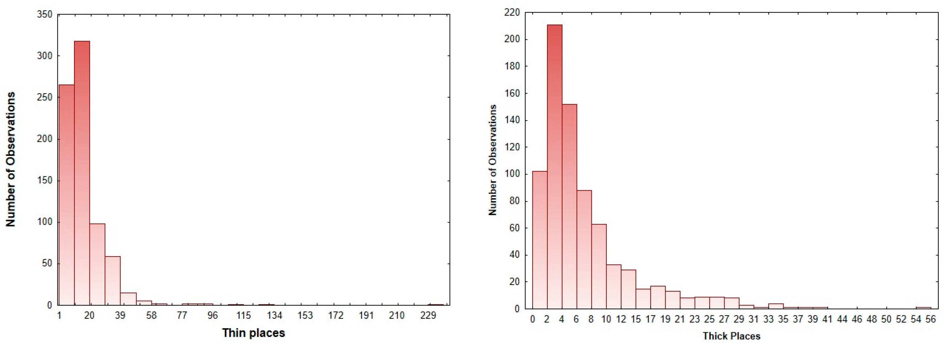
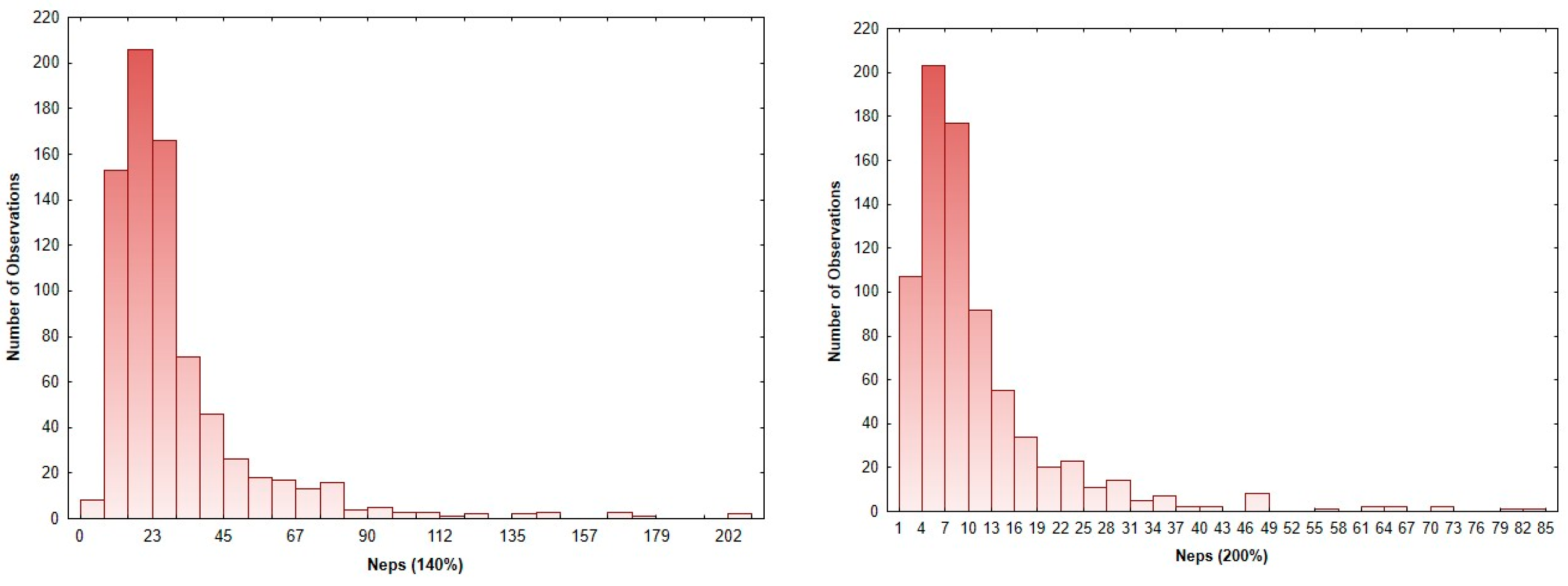
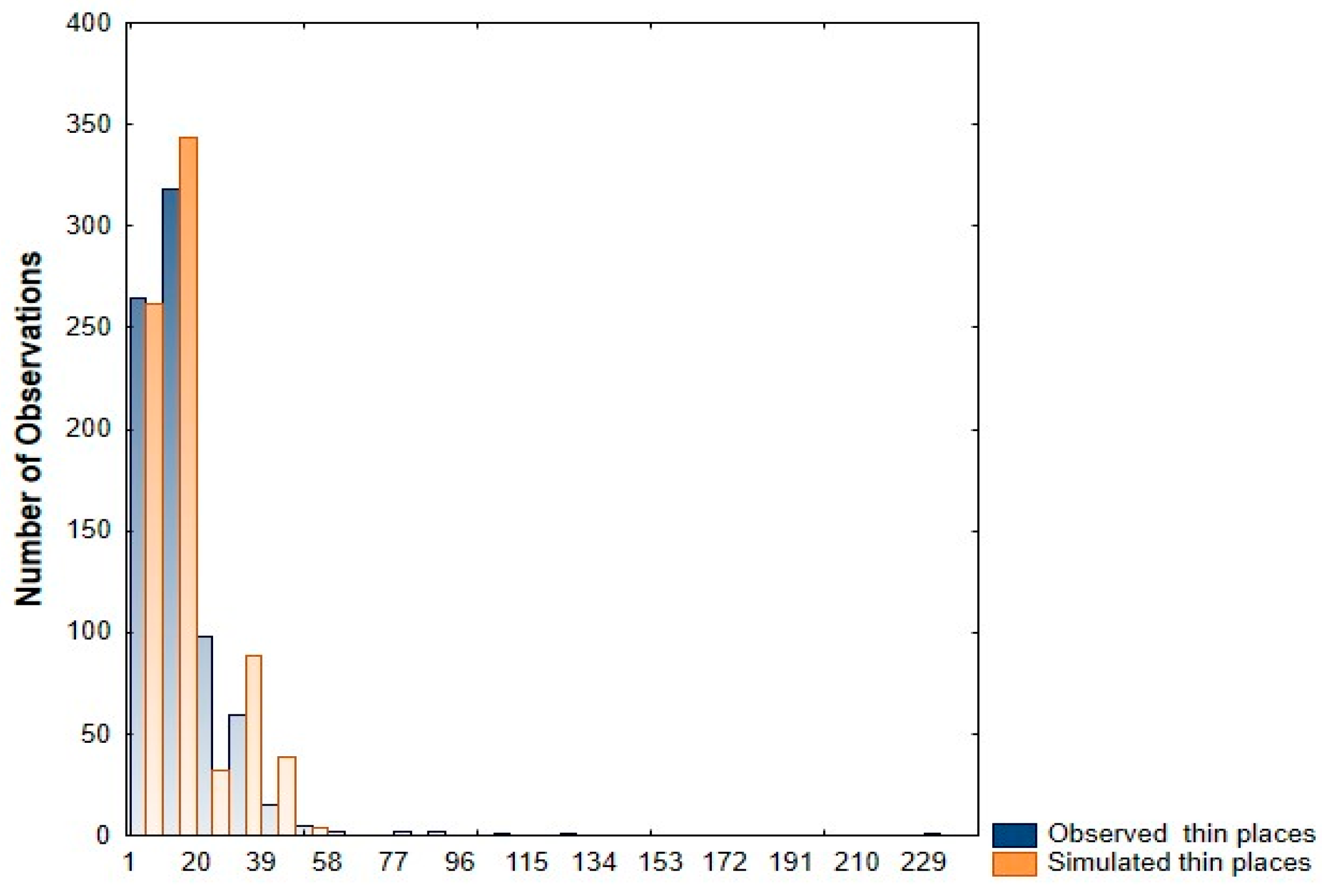
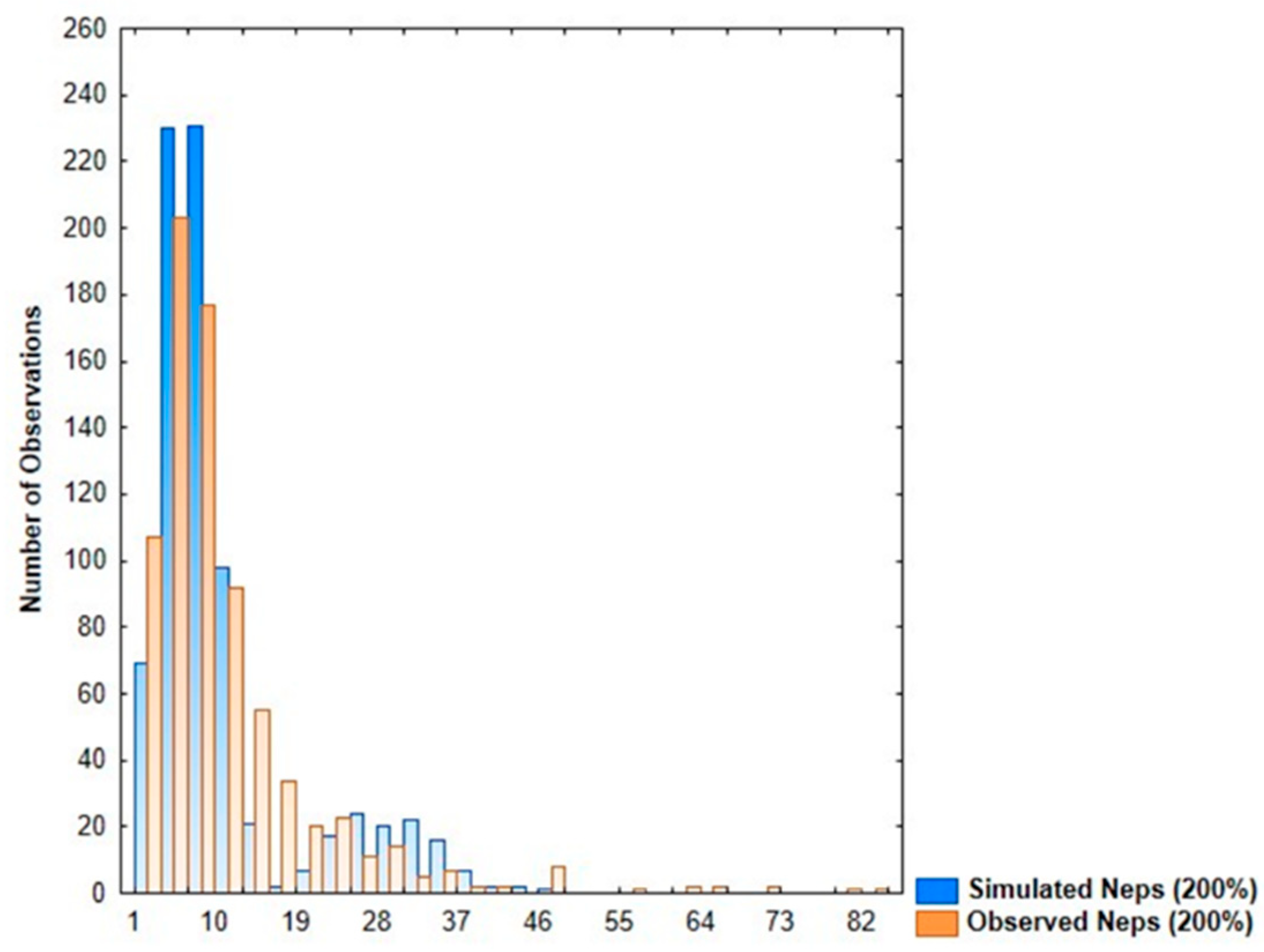
3.1. Distribution Fitting of Yarn Imperfection Parameters

The results of the chi-square (${\chi }^2)$ goodness-of-fit test revealed that the observed data for thin places, thick places, and neps in the yarn samples did not conform to standard single distributions, such as binomial, geometric, or Poisson distributions. This finding strongly suggests that these parameters follow a more complex, heterogeneous pattern that can be better described using mixture models.

The histograms of the observed data further supported this conclusion by showing multiple peaks, indicative of an underlying mixture of distributions (Figure 1 and Figure 2).

Poisson mixture distribution was applied to model each dataset, with parameters estimated using the EM algorithm. The results of these estimations are summarized in

Table 3. Poisson mixture distribution parameters for each dataset.

Data	k	Proportions			Poisson Mixture Distribution Parameters			Selection Criteria
		${\mathbf{w}}_1$	${\mathbf{w}}_2$	${\mathbf{w}}_3$	${\mathsf{\lambda }}_1$	${\mathsf{\lambda }}_2$	${\mathsf{\lambda }}_3$	AIC	BIC	LL
Thin 40%	2	0.79	0.21	-	11.64	35.68	-	6934.28	6948.21	−3464.14
Thick 50%	3	0.073	0.21	0.72	25.76	11.80	4.42	4466.874	4490.099	4634.936
Neps 140%	3	0.71	0.23	0.06	19.31	45.89	107.06	7152.014	7175.239	7224.290
Neps 200%	2	0.15	0.85	-	30.80	8.25	-	5508.402	5522.338	5550.933

. The proportions and parameters of each Poisson mixture distribution were calculated using the Flexmix (version 2.3-19) package in the R (version 4.1.0) programming environment.

These results indicate that a two-component Poisson mixture distribution is sufficient for modeling thin places and neps (200%), while a three-component distribution better fits the data for thick places and neps (140%).

The estimated proportions and distribution parameters provide valuable insights into the occurrence of imperfections in the yarn.

• Thin places: The analysis identifies a high-proportion component (0.79) with a mean of 11.64. This indicates that most thin places are relatively minor deviations, with occasional severe irregularities (mean of 35.68).
• Thick places: The three components represent varying degrees of thickness irregularities, with the largest proportion (0.72) attributed to minor variations. The presence of more extreme thick places (means of 25.76 and 11.80) highlights potential process inefficiencies, potentially attributable to such factors as inappropriate tension settings or irregular fiber feeding.
• Neps: The data indicate that across both the 140% and 200% sensitivity levels for neps, there is a mixture of mild, moderate, and severe instances. The extreme values identified could be indicative of inconsistencies in fiber preparation or during spinning processes. Such irregularities are often linked to fiber contamination or processing errors that can lead to significant adverse effects on the overall fabric quality.

The validity of the Poisson mixture models was evaluated through both visual inspection and statistical testing using the Mann–Whitney U test. The same dataset used for parameter estimation was also used for this evaluation. A close agreement between the observed data and the fitted models was observed, as evidenced by the overlay of histograms of the observed data with the probability density functions derived from the estimated models. These visual comparisons are presented for thin places, thick places, and both neps (140% and 200%) in Figure 3, Figure 4, Figure 5 and Figure 6, respectively.

An even more reliable method for determining whether the observed data and the data generated from the distribution come from the same population is to perform the Mann–Whitney U test.

The null hypothesis (H₀) of the Mann–Whitney U test suggests that the two groups are drawn from the same population. In other words, it proposes that the two independent groups are homogeneous and follow the same distribution. The alternative hypothesis (H₁), which is tested against the null hypothesis, suggests that the distribution of data in the first group differs from that of the second group [37]. Thus, the hypotheses are as follows:

H₀. 

There is no significant difference between the distribution of the observed dataset and the Poisson mixture distribution.

H₁. 

There is a significant difference between the distribution of the observed dataset and the Poisson mixture distribution.

According to the Mann–Whitney U test results, all examined datasets produced p-values greater than 0.05. Specifically, the p-value was 0.26 for the thin places dataset, 0.49 for the thick places dataset, 0.75 for the neps 200% dataset, and 0.30 for the neps 140% dataset. These findings confirm that the Poisson mixture distributions effectively represent each dataset.

The Poisson mixture parameters provided in Table 3 were applied in conjunction with Equations (30) and (34) to compute the mean and standard deviation for thin places, thick places, and neps. The computed values exhibit strong concordance with the observed data for elongation and tensile strength, as presented in

Table 4. Mean and standard deviation of yarn imperfection parameters: observed data vs. Poisson mixture model data.

Quality Parameters	Observed Data		PMM Data
	Mean	Standard Dev.	Mean	Standard Dev.
Thin Places (40%)	16.63	14.83	16.68	10.60
Thick Places (50%)	7.52	6.67	7.54	6.51
Neps (140%)	29.70	23.61	30.68	22.92
Neps (200%)	11.55	9.61	11.63	8.74

. Thus, the strong agreement between the observed and modeled mean and standard deviation values further strengthens the reliability of the proposed Poisson mixture models.

After establishing the validity of the mixed distribution using the Mann–Whitney U test, the probability functions were obtained by substituting the Poisson mixture distribution parameters provided in Table 3 into Equation (2).

$${f(x)}_{thin}=0.79{\displaystyle \frac{{11.64}^x{e}^{-11.64}}{x!}}+0.21 {\displaystyle \frac{{35.68}^x{e}^{-35.68}}{x!}}$$

(68)

$${f(x)}_{thick}=0.073{\displaystyle \frac{{25.76}^x{e}^{-25.76}}{x!}}+0.21{\displaystyle \frac{{11.8}^x{e}^{-11.8}}{x!}}+0.72{\displaystyle \frac{{4.42}^x{e}^{-4.42}}{x!}}$$

(69)

$${f(x)}_{neps140}=0.71{\displaystyle \frac{{19.31}^x{e}^{-19.31}}{x!}}+0.23{\displaystyle \frac{{45.89}^x{e}^{-45.89}}{x!}}+0.06{\displaystyle \frac{{107.06}^x{e}^{-107.06}}{x!}}$$

(70)

$${f(x)}_{neps200}=0.15{\displaystyle \frac{{30.80}^x{e}^{-30.80}}{x!}}+0.85 {\displaystyle \frac{{8.25}^x{e}^{-8.25}}{x!}}$$

(71)

Determining the probability distribution function of thin places (Equation (68)), thick places (Equation (69)), and neps (Equations (70) and (71)) provides significant benefits for optimizing quality control and enhancing production efficiency. The derived probability functions offer predictive insight into the likelihood of yarn imperfections, enabling more proactive and data-driven quality control practices. These models can be directly compared against specification limits defined for each imperfection type to estimate the probability of conformance. This capability can significantly enhance quality control mechanisms in production processes.

To further evaluate the practical applicability of the proposed Poisson mixture models in quality control, conformance probabilities were calculated based on upper specification limits provided by the yarn manufacturer. These limits reflect the quality thresholds expected by the company’s customers for each defect type—namely, thin places (≤35), thick places (≤10), neps at 140% sensitivity (≤127), and neps at 200% sensitivity (≤26). The probability of conformance was computed as the cumulative probability $P\left(X\le spec.\right)$ under the respective mixture distribution functions (Equations (69)–(72)).

The results reveal that the estimated conformance probabilities are 0.923 for thin places, 0.793 for thick places, 0.998 for neps at 140%, and 0.892 for neps at 200%. These values indicate that, while neps at 140% and thin place imperfections are largely within acceptable bounds, neps at 200% and thick places exhibit relatively lower conformance levels. This insight can help quality engineers prioritize improvement efforts and implement corrective measures more effectively for specific defect categories.

Thus, understanding the probability distribution enables predictive insights, allowing for proactive measures to prevent similar irregularities in future production batches. Such foresight is instrumental in minimizing potential quality issues, thereby fostering higher levels of customer satisfaction. Furthermore, integration of these models into real-time quality monitoring systems allows for instant alerts when defect probabilities exceed tolerable bounds. This capability ensures timely intervention and minimizes the occurrence of defective batches.

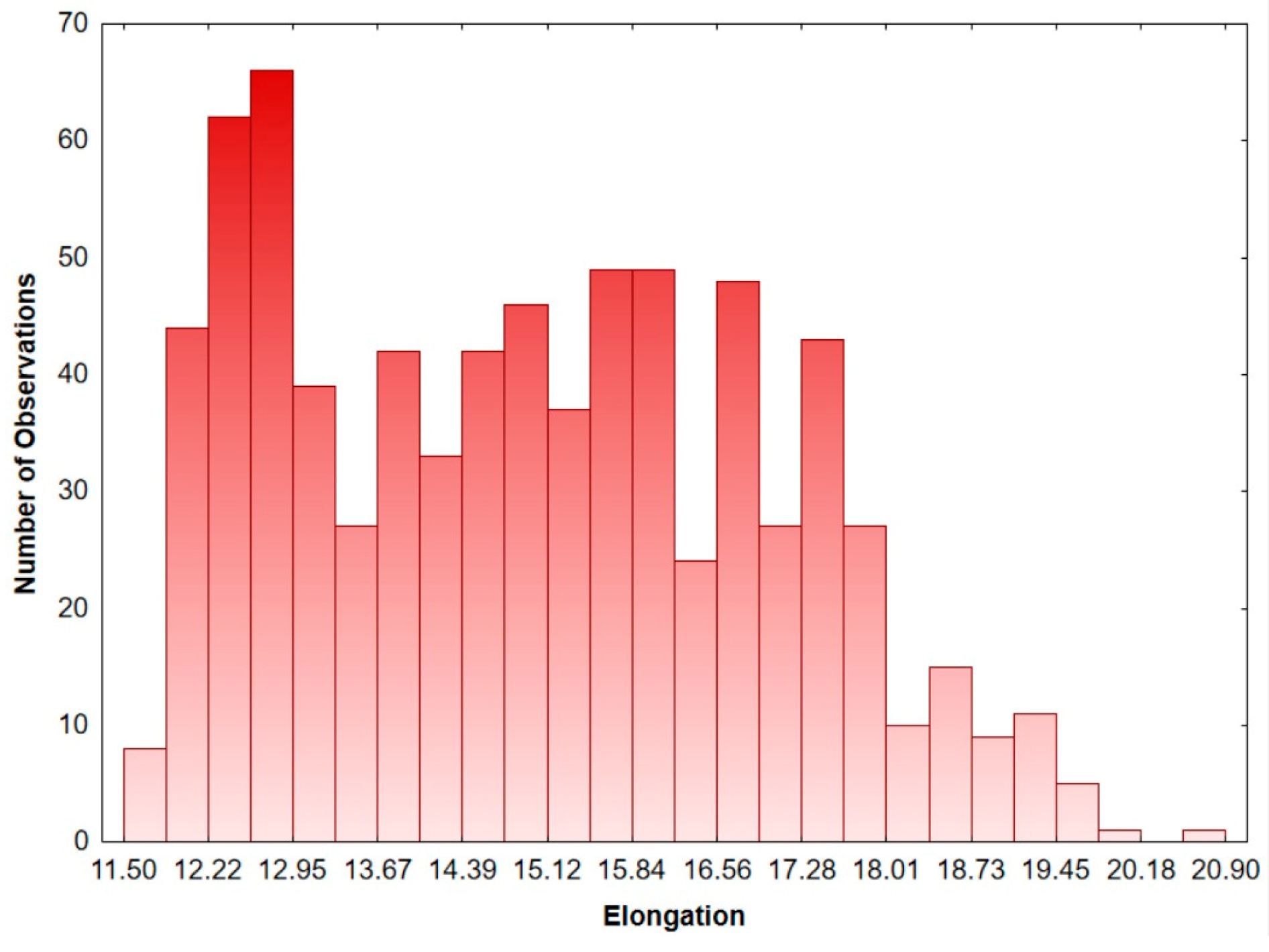
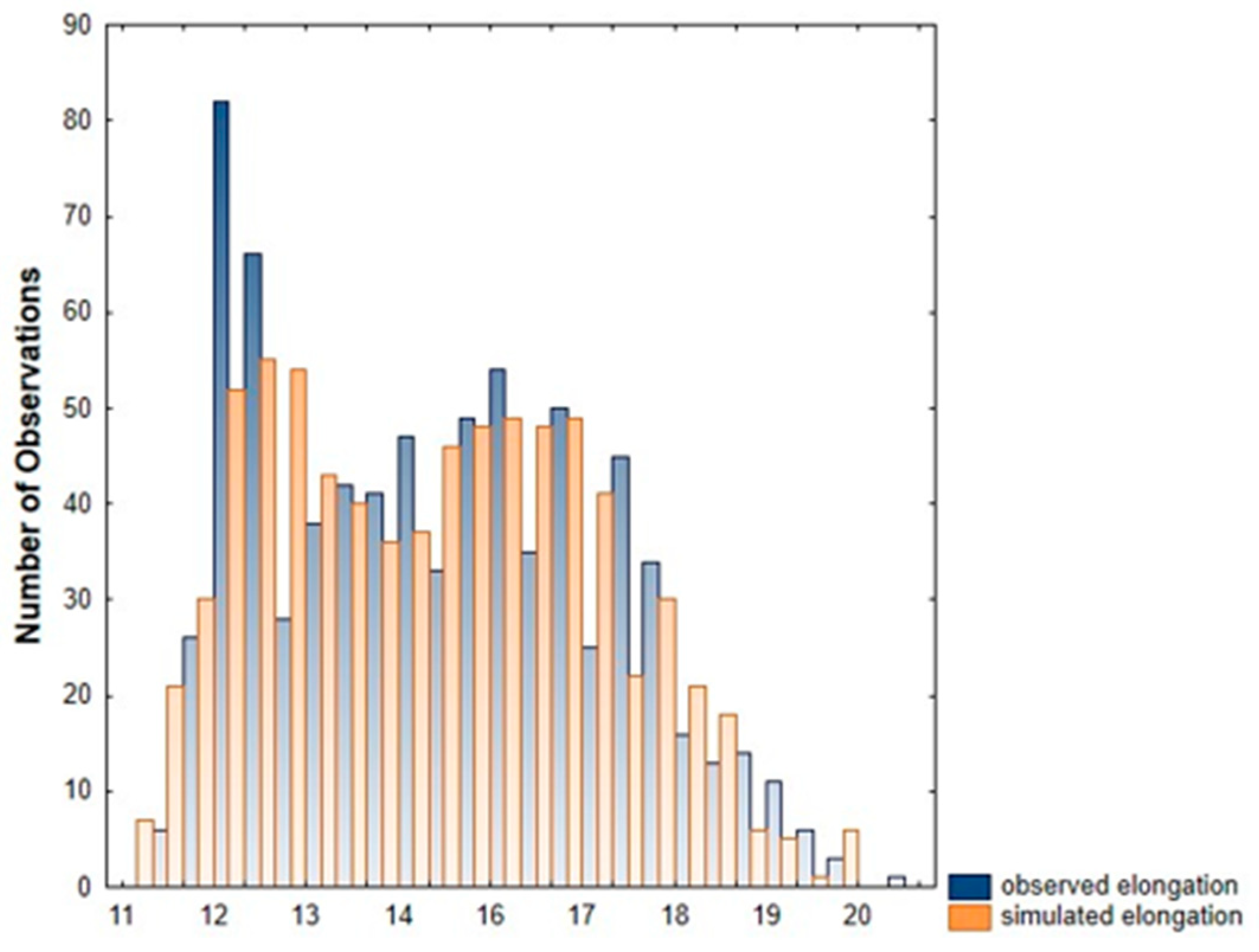
3.2. Distribution Fitting of Yarn Mechanical Properties

Following the comprehensive evaluation of yarn imperfection parameters, the subsequent analysis focused on investigating the mechanical properties of the yarn, particularly tensile strength (tenacity) and elongation. This investigation was conducted under the assumption that the underlying data might follow a specific statistical distribution. However, the application of the chi-square goodness-of-fit test indicated that the datasets related to these mechanical properties did not conform to any single distribution, suggesting a more complex underlying structure in the observed data.

Figure 7 and Figure 8 illustrate the histogram of the respective datasets, revealing multiple peaks, which suggest that the data may follow a mixed distribution.

Each dataset was modeled using gamma mixture distributions, with parameters estimated through the EM algorithm. A summary of these estimation results is provided in

Table 5. Gamma mixture distribution parameters for each dataset.

Data	k	Proportions		Gamma Mixture Distribution Parameters		Selection Criteria
		${\mathsf{\pi }}_1$	${\mathsf{\pi }}_2$	$({\mathit{\alpha }}_1,{\mathit{\beta }}_1)$	$({\mathit{\alpha }}_2,{\mathit{\beta }}_2)$	AIC	BIC	LL
Elongation	2	0.33	0.67	(320, 0.04)	(110, 0.146)	3121.86	3145.06	−1555.93
Tensile Str.	2	0.52	0.48	(120, 0.17)	(280, 0.09)	3825.70	3848.90	−1907.85

. The proportions and parameters of each gamma mixture distribution were determined using the Flexmix package in the R programming environment.

A comparison of the histograms representing the observed data with the probability density functions derived from the fitted gamma mixture models is illustrated in Figure 9 and Figure 10, which clearly demonstrates a strong degree of agreement between the empirical data and the models. Such visual consistency underscores the assertion that the proposed gamma mixture models adequately capture the underlying distribution of the observed data for both tensile strength and elongation.

In addition to visual assessments, the Mann–Whitney U test was employed to statistically analyze the differences between the observed and modeled distributions. The results of this non-parametric test indicated that all examined datasets produced p-values exceeding the conventional threshold of 0.05. Specifically, the p-value for the tensile strength dataset was 0.69, while the elongation dataset produced a p-value of 0.40. These findings imply that there are no significant differences between the distributions of the observed data and those modeled by the gamma mixture framework.

The parameters of the gamma mixture models, detailed in Table 5, were employed alongside Equations (64) and (66) to calculate the mean and standard deviation for both elongation and tensile strength. The computed values from these equations indicate a close alignment with the observed data, which are documented in

Table 6. Mean and standard deviation of elongation and tensile strength: observed data vs. gamma mixture model data.

Quality Parameters	Observed Data		GMM Data
	Mean	Standard Dev.	Mean	Standard Dev.
Elongation	14.97	2.03	14.98	2.01
Tensile strength	22.89	3.25	22.86	3.35

. This congruence reinforces the validity of the gamma mixture models in accurately capturing the statistical characteristics of the underlying datasets.

Following the validation of the mixed distribution, the corresponding probability functions for elongation and tensile strength were derived by substituting the gamma mixture distribution parameters from Table 5 into Equation (35). The resulting probability density functions are given in Equations (72) and (73).

$${f(x)}_{elongation}=0.33{\displaystyle \frac{{0.04}^{320}{x}^{319}{e}^{-0.04x}}{{\int }_0^{\infty }{t}^{319}{e}^{-t}dt}}+0.67{\displaystyle \frac{{0.146}^{110}{x^{109}e}^{-0.146x}}{{\int }_0^{\infty }{t}^{109}{e}^{-t}dt)}}$$

(72)

$${f\left(x\right)}_{tstrength}=0.52{\displaystyle \frac{{0.17}^{120}{x}^{119}{e}^{-0.17x}}{{\int }_0^{\infty }{t}^{119}{e}^{-t}dt}}+0.48{\displaystyle \frac{{0.09}^{280}{x^{279}e}^{-0.09x}}{{\int }_0^{\infty }{t}^{279}{e}^{-t}dt)}}$$

(73)

In spinning mills, the variability in elongation and tensile strength directly affects the performance characteristics of the produced yarns. Establishing the probability density function for these properties is critical for effectively modeling the statistical behavior of elongation and tensile strength, providing insights that can be leveraged for quality control and predictive analysis in yarn production processes.

In summary, employing a suitable FMM for both yarn irregularity and mechanical properties offers several key advantages, as follows:

• Prediction and control: The obtained probability density functions allow for the prediction of the likelihood of specific parameter values occurring in future yarn production. This predictive capability is crucial for process control, enabling adjustments to maintain desired quality standards. When integrated into real-time quality monitoring systems, this predictive capability enables timely interventions by triggering alerts when the probability of conformance falls below critical thresholds.
• Modeling and simulation: Probability functions can be integrated into more complex models and simulations of textile manufacturing processes. This facilitates virtual experimentation and optimization, reducing reliance on costly and time-consuming physical trials.
• Risk assessment: The obtained probability density functions allow for a more precise evaluation of the risk associated with producing fabrics that do not meet predefined performance specifications. By quantifying the probability of conformance, manufacturers can assess the likelihood of deviation from quality standards in advance. This type of risk assessment is particularly crucial in high-performance applications—such as medical textiles, aerospace composites, or protective fabrics—where yarn failure could lead to severe functional or safety consequences.

4. Conclusions

This study demonstrates the effective application of finite mixed models for characterizing key yarn quality parameters in a 28/1 Ne ring-spun polyester/viscose yarn. By employing Poisson and gamma mixture distributions and using advanced statistical techniques, such as the EM algorithm, this research provides a robust framework for modeling the heterogeneity observed in yarn quality parameters. Moreover, the validation of the model using goodness-of-fit tests and the Mann–Whitney U test underscores the reliability of the proposed method.

The findings have significant implications for the textile industry. Understanding the probability distributions of quality parameters enables manufacturers to implement proactive quality control measures, optimize production processes, and predict irregularities in future batches. This approach not only reduces waste and production costs but also improves quality and customer satisfaction. These insights pave the way for future studies to explore mixture models in other aspects of textile production, such as in relation to fiber properties or a wider range of yarn types.

References

1. Bouguila, N.; Fan, W. Mixture Models and Applications; Springer: Berlin/Heidelberg, Germany, 2020; Volume 530. [Google Scholar]
2. Ng, S.-K. Mixture Modelling for Medical and Health Sciences; Chapman and Hall/CRC: Boca Raton, FL, USA, 2019. [Google Scholar]
3. Yu, J.; Qin, S.J. Multiway Gaussian mixture model based multiphase batch process monitoring. Ind. Eng. Chem. Res. 2009, 48, 8585–8594. [Google Scholar] [CrossRef]
4. Hafemeister, C.; Costa, I.G.; Schönhuth, A.; Schliep, A. Classifying short gene expression time-courses with Bayesian estimation of piecewise constant functions. Bioinformatics 2011, 27, 946–952. [Google Scholar] [CrossRef] [PubMed]
5. Neema, I.; Böhning, D. Improved methods for surveying and monitoring crimes through likelihood based cluster analysis. Int. J. Criminol. Sociol. Theory 2010, 3, 477–495. [Google Scholar]
6. Chambers, S.K.; Ng, S.K.; Baade, P.; Aitken, J.F.; Hyde, M.K.; Wittert, G.; Frydenberg, M.; Dunn, J. Trajectories of quality of life, life satisfaction, and psychological adjustment after prostate cancer. Psycho-Oncology 2017, 26, 1576–1585. [Google Scholar] [CrossRef] [PubMed]
7. Wessman, J.; Paunio, T.; Tuulio-Henriksson, A.; Koivisto, M.; Partonen, T.; Suvisaari, J.; Turunen, J.A.; Wedenoja, J.; Hennah, W.; Pietiläinen, O.P. Mixture model clustering of phenotype features reveals evidence for association of DTNBP1 to a specific subtype of schizophrenia. Biol. Psychiatry 2009, 66, 990–996. [Google Scholar] [CrossRef]
8. Palardy, G.J.; Vermunt, J.K. Multilevel growth mixture models for classifying groups. J. Educ. Behav. Stat. 2010, 35, 532–565. [Google Scholar] [CrossRef]
9. ElMoaqet, H.; Kim, J.; Tilbury, D.; Ramachandran, S.K.; Ryalat, M.; Chu, C.-H. Gaussian mixture models for detecting sleep apnea events using single oronasal airflow record. Appl. Sci. 2020, 10, 7889. [Google Scholar] [CrossRef]
10. Fahey, M.T.; Ferrari, P.; Slimani, N.; Vermunt, J.K.; White, I.R.; Hoffmann, K.; Wirfält, E.; Bamia, C.; Touvier, M.; Linseisen, J. Identifying dietary patterns using a normal mixture model: Application to the EPIC study. J. Epidemiol. Community Health 2012, 66, 89–94. [Google Scholar] [CrossRef]
11. Ji, Z.; Xia, Y.; Sun, Q.; Chen, Q.; Xia, D.; Feng, D.D. Fuzzy local Gaussian mixture model for brain MR image segmentation. IEEE Trans. Inf. Technol. Biomed. 2012, 16, 339–347. [Google Scholar]
12. Tentoni, S.; Astolfi, P.; De Pasquale, A.; Zonta, L.A. Birthweight by gestational age in preterm babies according to a Gaussian mixture model. BJOG Int. J. Obstet. Gynaecol. 2004, 111, 31–37. [Google Scholar] [CrossRef]
13. Sun, T.; Wen, Y.; Zhang, X.; Jia, B.; Zhou, M. Gaussian mixture model for marine reverberations. Appl. Sci. 2023, 13, 12063. [Google Scholar] [CrossRef]
14. Krifa, M. Fiber length distribution in cotton processing: A finite mixture distribution model. Text. Res. J. 2008, 78, 688–698. [Google Scholar] [CrossRef]
15. Cui, X.; Rodgers, J.; Cai, Y.; Li, L.; Belmasrour, R.; Pang, S.-S. Obtaining cotton fiber length distributions from the beard test method Part 1-Theoretical distributions related to the beard method. J. Cotton Sci. 2009, 13, 265–273. [Google Scholar]
16. Belmasrour, R.; Li, L.; Cui, X.; Cai, Y.; Rodgers, J. Obtaining cotton fiber length distributions from the beard test method. Part 1—A new approach through PLS Regression. J. Cotton Sci. 2011, 15, 73–79. [Google Scholar]
17. Lin, Q.; Xing, M.; Oxenham, W.; Yu, C. Generation of cotton fiber length probability density function with length measures. J. Text. Inst. 2012, 103, 225–230. [Google Scholar] [CrossRef]
18. Kuang, X.; Hu, Y.; Yang, J.; Yu, C. Application of finite mixture model in cotton fiber length probability distribution. J. Text. Inst. 2015, 106, 146–151. [Google Scholar] [CrossRef]
19. Repon, M.R.; Al Mamun, R.; Reza, S.; Das, M.K.; Islam, T. Effect of spinning parameters on thick, thin places and neps of rotor spun yarn. J. Text. Sci. Technol. 2016, 2, 47–55. [Google Scholar] [CrossRef]
20. Mwasıagı, J.; Mırembel, J. Influence of Spinning Parameters on thin and thick Places of rotor spun yarns. Int. J. Comput. Exp. Sci. Eng. 2018, 4, 1–7. [Google Scholar] [CrossRef]
21. Ozcelik, G.; Kirtay, E.; Derici, I.M. Examination of fiber neps count during yarn manufacturing. In Proceedings of the Beltwide Cotton Conference, New Orleans, LA, USA, 4–7 January 2005; pp. 2229–2235. [Google Scholar]
22. Frydrych, I.; Matusiak, M. Predicting the Nep Number in Cotton Yarn—Determining the Critical Nep Size. Text. Res. J. 2002, 72, 917–923. [Google Scholar] [CrossRef]
23. Nath, J.M.; Shukla, S.; Patil, P. Neps in cotton. J. Cotton Res. Dev. 2015, 29, 329–332. [Google Scholar]
24. Habib, A.; Olgun, Y.; Babaarslan, O. Development of dual-core spun yarn using different filaments as a core and its impact on denim fabric properties. Text. Leather Rev. 2024, 7, 534–549. [Google Scholar] [CrossRef]
25. Kebabcı, M.; Babaarslan, O.; Hacıoğulları, S.Ö.; Telli, A. The effect of drawing ratio and cross-sectional shapes on the properties of polypropylene CF and BCF yarns. Tekst. Mühendis 2015, 22, 46–53. [Google Scholar] [CrossRef]
26. Lemmi, T.S.; Barburski, M.; Kabziński, A.; Frukacz, K. Effect of thermal aging on the mechanical properties of high tenacity polyester yarn. Materials 2021, 14, 1666. [Google Scholar] [CrossRef] [PubMed]
27. Li, Z.; Meng, C.; Zhou, J.; Li, Z.; Ding, J.; Liu, F.; Yu, C. Characterization and control of oxidized cellulose in ramie fibers during oxidative degumming. Text. Res. J. 2017, 87, 1828–1840. [Google Scholar] [CrossRef]
28. Liu, Y.; Thibodeaux, D.; Gamble, G.; Rodgers, J. Preliminary study of relating cotton fiber tenacity and elongation with crystallinity. Text. Res. J. 2014, 84, 1829–1839. [Google Scholar] [CrossRef]
29. Široká, B.; Manian, A.P.; Noisternig, M.F.; Henniges, U.; Kostic, M.; Potthast, A.; Griesser, U.J.; Bechtold, T. Wash–dry cycle induced changes in low-ordered parts of regenerated cellulosic fibers. J. Appl. Polym. Sci. 2012, 126, E397–E408. [Google Scholar] [CrossRef]
30. Upreti, M.; Jahan, S. Study the effect of scouring time on Grewia asiatica (Phalsa) fibres properties. J. Appl. Nat. Sci. 2017, 9, 1388. [Google Scholar] [CrossRef]
31. Maiti, S.; Islam, M.R.; Uddin, M.A.; Afroj, S.; Eichhorn, S.J.; Karim, N. Sustainable fiber-reinforced composites: A review. Adv. Sustain. Syst. 2022, 6, 2200258. [Google Scholar] [CrossRef]
32. Gorjanc, D.S.; Bizjak, M. The influence of constructional parameters on deformability of elastic cotton fabrics. J. Eng. Fibers Fabr. 2014, 9, 155892501400900106. [Google Scholar] [CrossRef]
33. Dempster, A.P.; Laird, N.M.; Rubin, D.B. Maximum likelihood from incomplete data via the EM algorithm. J. R. Stat. Soc. Ser. B Methodol. 1977, 39, 1–22. [Google Scholar] [CrossRef]
34. Ghojogh, B.; Ghojogh, A.; Crowley, M.; Karray, F. Fitting a mixture distribution to data: Tutorial. arXiv 2019, arXiv:1901.06708. [Google Scholar]
35. Almhana, J.; Liu, Z.; Choulakian, V.; McGorman, R. A recursive algorithm for gamma mixture models. In Proceedings of the 2006 IEEE International Conference on Communications, Istanbul, Turkey, 11–15 June 2006; pp. 197–202. [Google Scholar]
36. Liu, Z.; Almhana, J.; Choulakian, V.; McGorman, R. Traffic modeling with gamma mixtures and dynamical bandwidth provisioning. In Proceedings of the 4th Annual Communication Networks and Services Research Conference (CNSR’06), Moncton, NB, Canada, 24–25 May 2006; pp. 8–130. [Google Scholar]
37. Nachar, N. The Mann-Whitney U: A test for assessing whether two independent samples come from the same distribution. Tutor. Quant. Methods Psychol. 2008, 4, 13–20. [Google Scholar] [CrossRef]
Figure 1. Histograms of thin and thick places.
Applsci 15 06407 g001
Figure 2. Histograms of neps (140%, 200%).
Applsci 15 06407 g002
Figure 3. Thin places: histogram of observed data and fitted Poisson mixture data.
Applsci 15 06407 g003
Figure 4. Thick places: histogram of observed data and fitted Poisson mixture data.
Applsci 15 06407 g004
Figure 5. Neps (%140): histogram of observed data and fitted Poisson mixture data.
Applsci 15 06407 g005
Figure 6. Neps (%200): histogram of observed data and fitted Poisson mixture data.
Applsci 15 06407 g006
Figure 7. Histogram of elongation (%).
Applsci 15 06407 g007
Figure 8. Histogram of tensile strength (cN/tex).
Applsci 15 06407 g008
Figure 9. Tensile strength observed data and fitted gamma mixture data.
Applsci 15 06407 g009
Figure 10. Elongation observed data and fitted gamma mixture data.
Applsci 15 06407 g010