Comparative Experimental Study on the Dynamic and Static Stiffness of Sandy Soils Utilizing Alpan’s Empirical Approach


Abstract
1. Introduction
2. Materials and Test Methods
2.1. Materials
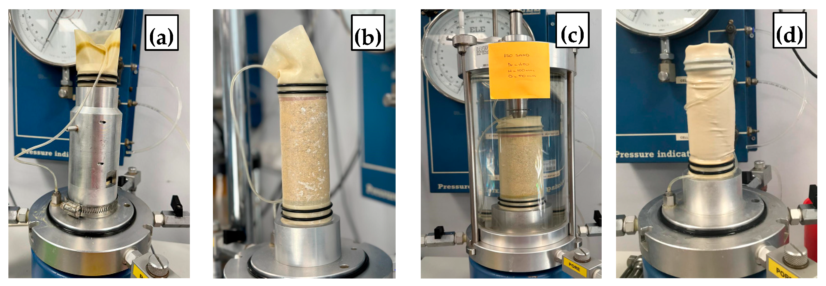
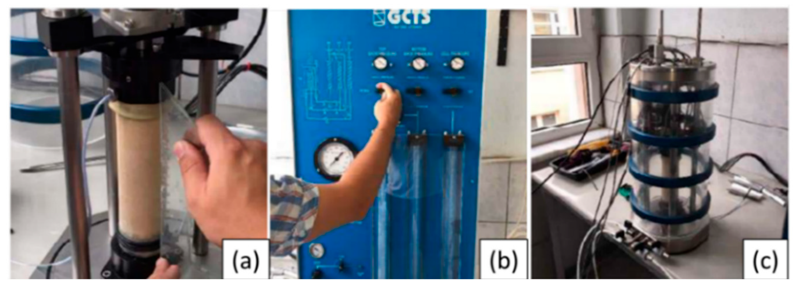
2.2. Test Methods
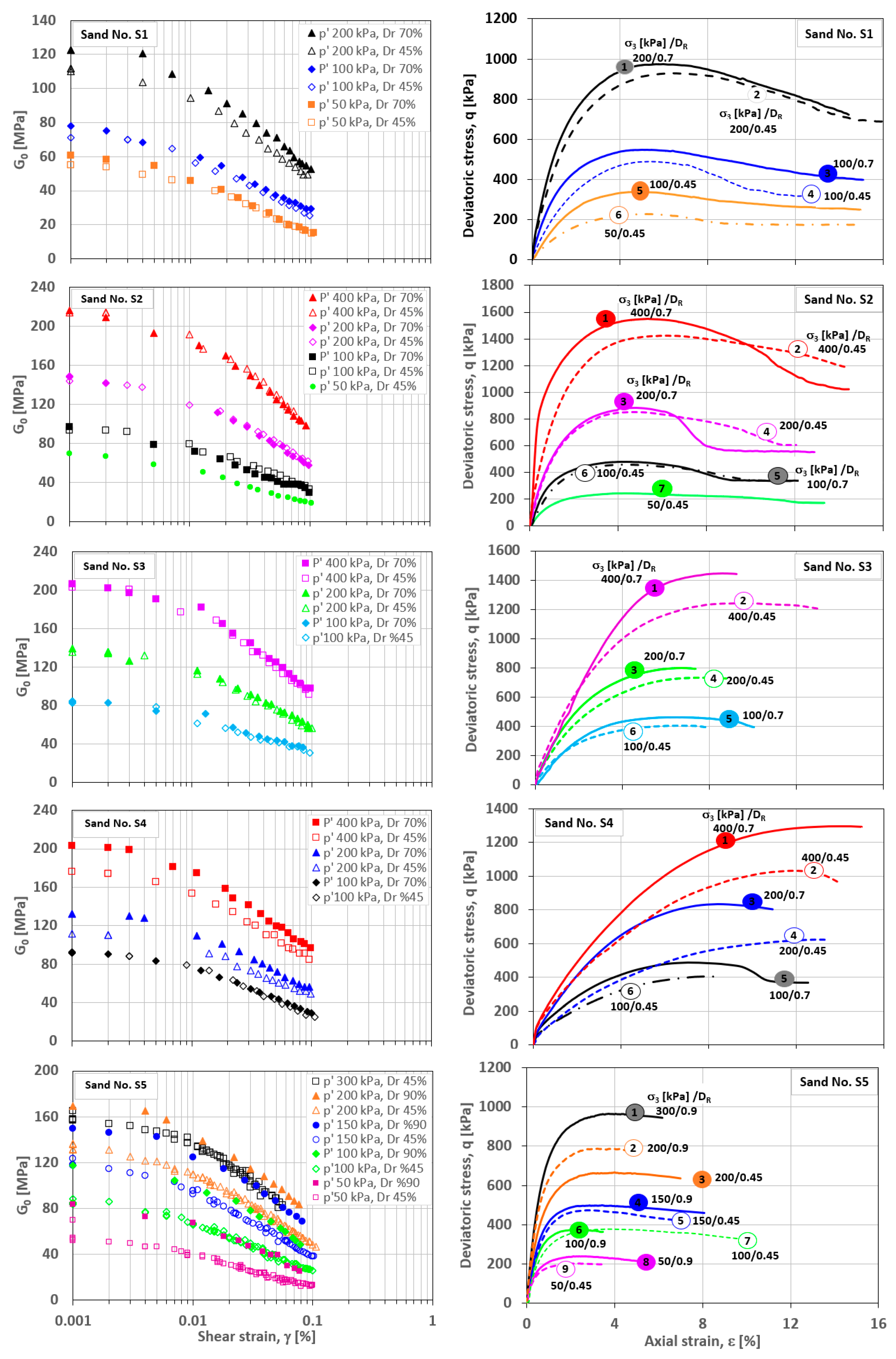
3. Results and Discussion
4. Concluding Remarks
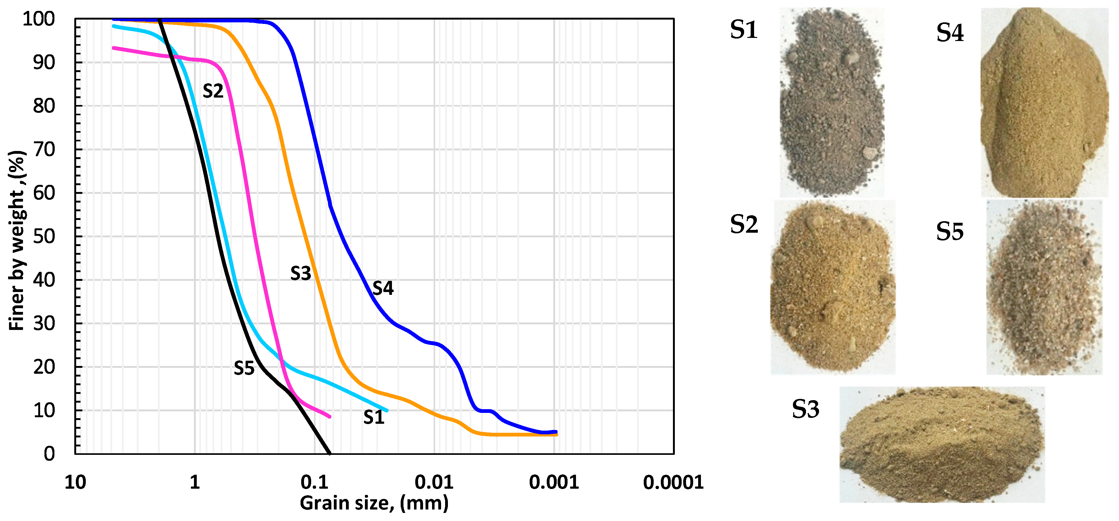
- This study examines sands classified as fine sand “SC” (S1 and S3) and well graded “SW” (S2, S4 and S5) according to the Unified Soil Classification System (USCS). These soils were tested with varying fine content (FC = 0–45%) and different levels of relative density (DR = 45% and DR = 70–90%). Therefore, the results obtained are valid for sandy soil with similar properties to the tested specimens.
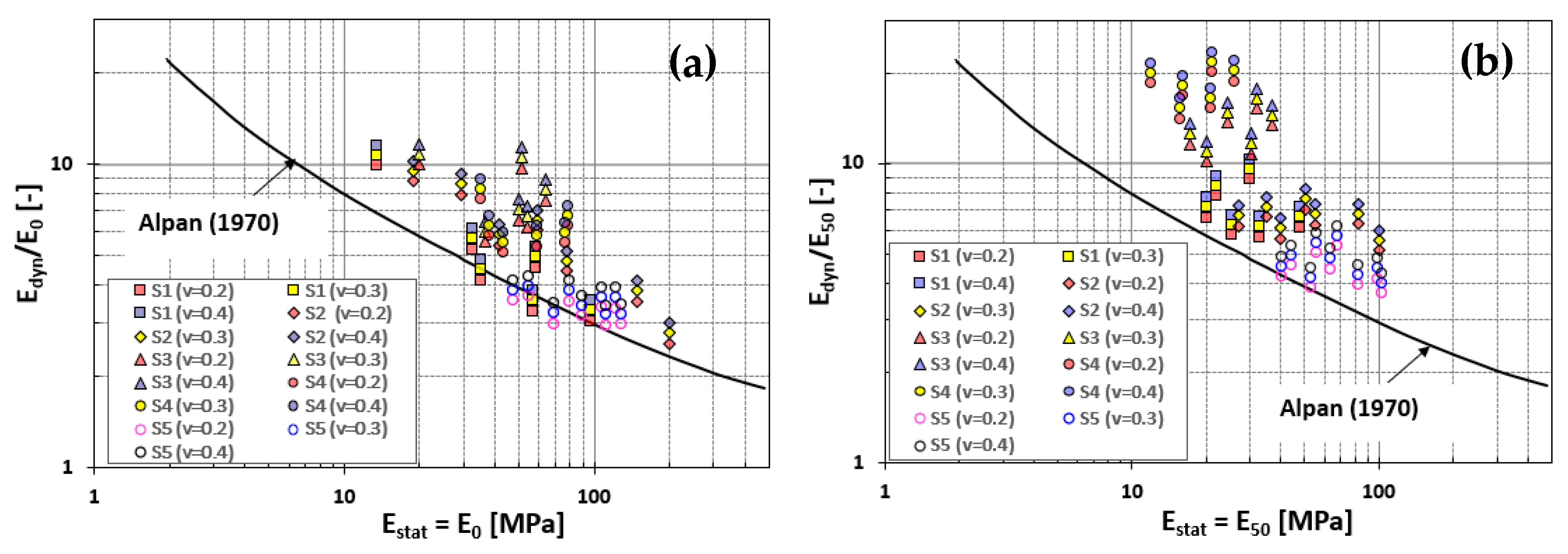
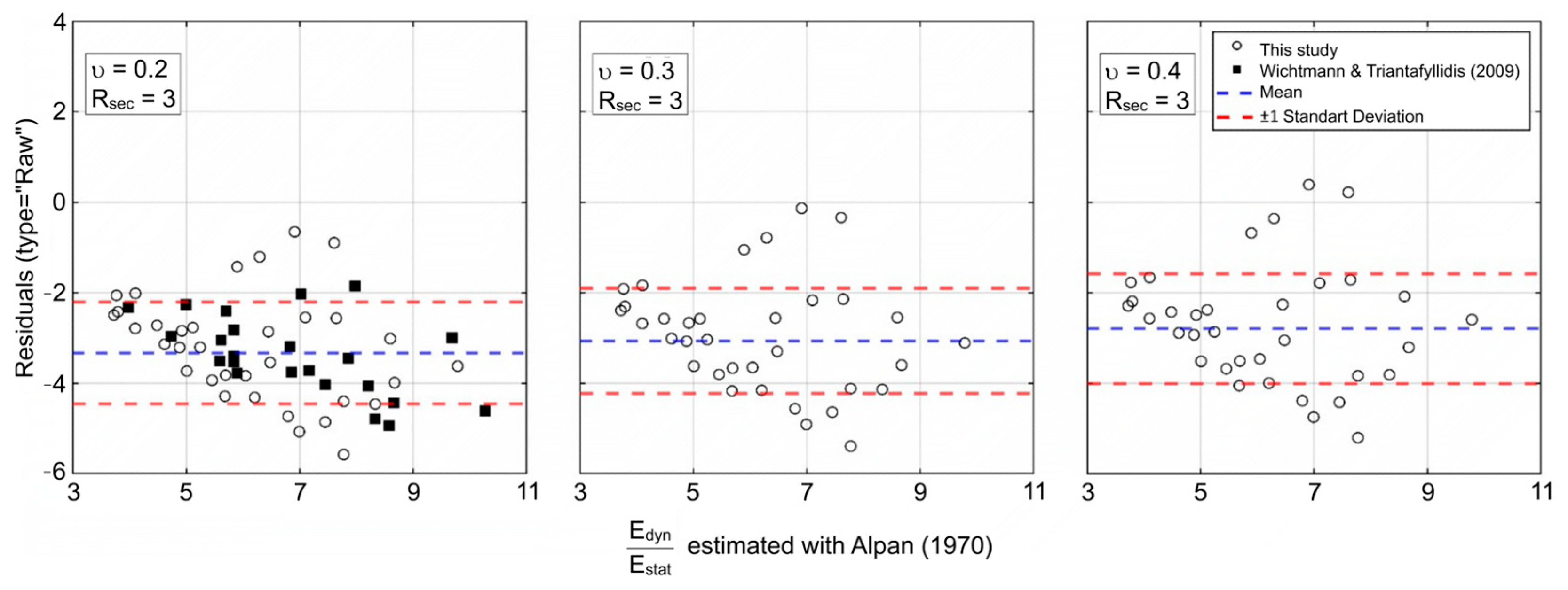
- The measured Edyn/Estat values are generally underestimated by the Alpan approach. When Poisson’s ratio is assumed to be small, the Alpan curve is approximated more closely. The results reveal that Poisson’s ratio significantly affects Edyn and hence the Edyn/Estat ratio.
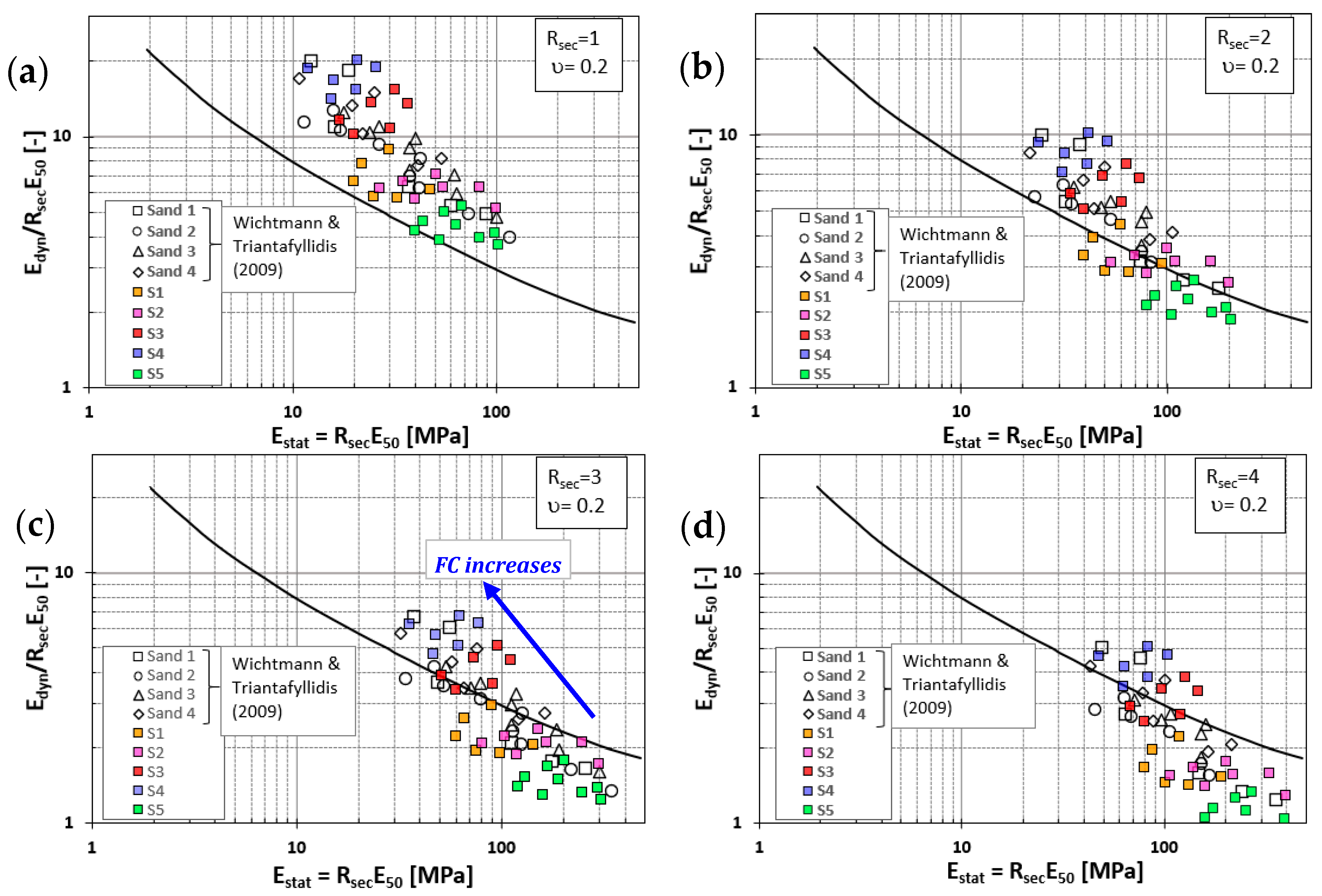
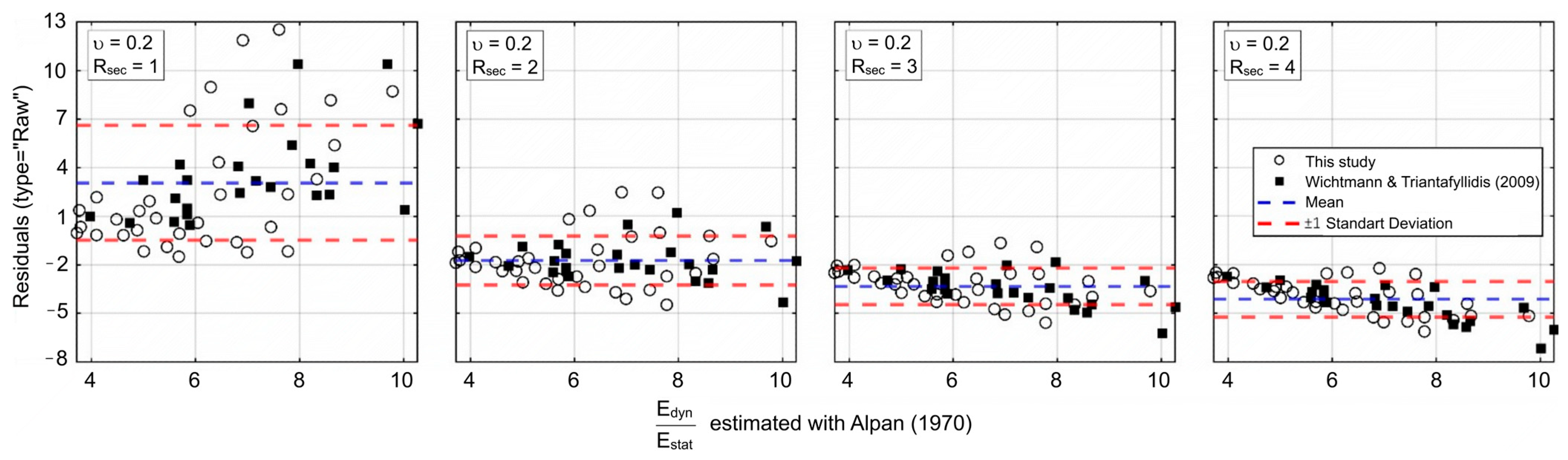
- The ratio between dynamic and static modulus as proposed by Alpan, the static elastic modulus (Estat) is not explicitly defined. The coefficient Rsec = Estat/E50 was introduced that Estat is a multiple of E50. Test results revealed the best agreement between dynamic and static stiffness ratio (Edyn/Estat) and static modulus of elasticity (Estat) for Rsec = 2 (when v is assumed 0.2). Statistical error analyses support this finding.
- According to the experimental results, it is safe to say that Alpan’s empirical approach is still valid when the values of Poisson’s ratio and Estat in the small deformation region are used. Ref. [3] diagram was found to be practical and appropriate when both static and dynamic tests were not performed on a soil.
- Since there are limited studies on Edyn/Estat ratio in the literature, it is thought that the findings in this paper will contribute to engineers and researchers. However, this work would also assist engineers in selecting appropriate stiffness parameters for calibrating constitutive models.
- It is observed that Edyn/Estat increases as the fine content increases. This and the updating of the mathematical expression originally proposed by [3] through new index properties (such as Cu and D50), confining stress and relative density are the subject of ongoing research.
Author Contributions
Funding
Institutional Review Board Statement
Informed Consent Statement
Data Availability Statement
Acknowledgments
Conflicts of Interest
References
- Jiang, S. Study on the Dynamic Characteristics of Solidified Silt Under Dynamic Load. Vibroengineering Procedia 2019, 27, 24–29. [Google Scholar] [CrossRef]
- Liu, S.; Li, J.; Ji, X.; Fang, Y. Influence of Root Distribution Patterns on Soil Dynamic Characteristics. Sci. Rep. 2022, 12, 13448. [Google Scholar] [CrossRef] [PubMed]
- Alpan, I. The geotechnical properties of soils. Earth-Sci. Rev. 1970, 6, 5–49. [Google Scholar] [CrossRef]
- Kelvin, W.T.B. On the elasticity and viscosity of metals. Proc. R. Soc. Lond. 1865, 14, 289–297. [Google Scholar]
- Voigt, W. Ueber innere Reibung fester Körper, insbesondere der Metalle. Ann. Phys. 1892, 283, 671–693. [Google Scholar] [CrossRef]
- des Arbeitskreises, E. “Baugrunddynamik“. Deutsche Gesellschaft Für Geotechnik EV (Hrsg.); Ernst & Sohn: Berlin, Germany, 2002. [Google Scholar]
- Benz, T.; Vermeer, P.A. Discussion of On the Correlation of Oedometric and Dynamic Stiffness of Non-cohesive Soils by T. Wichtmann and Th. Triantafyllidis (Bautechnik 83(7), 2006). Bautechnik 2007, 84, 361–364. (In German) [Google Scholar]
- Wichtmann, T.; Triantafyllidis, T. On the correlation of “static” and “dynamic” stiffness moduli of non-cohesive soils. Bautechnik 2009, 86 (Suppl. S1), 28–39. [Google Scholar] [CrossRef]
- Öztoprak, S.; Işık, N.S.; Karaca, Ö.; Ocakbaşı, E.; Eyisüren, O.; Işık, M.F.; Bektaş, Ö.; Sargın, S.; Büyüksaraç, A.; Umu, S.U.; et al. Development of Corresponding Methods, Coefficients and Maps for Including the Bedrock Depth and Basin Effect Into the Design Response Spectrums Obtained from Earthquake Design Codes and Seismic Site Response Analyses (TÜBİTAK 1001 Project No. 121M760); The Scientific and Technological Research Council of Türkiye (TÜBİTAK): Ankara, Turkey, 2021.
- ASTM D6913-04; Test Methods for Particle-Size Distribution (Gradation) of Soils Using Sieve Analysis. ASTM International: West Conshohocken, PA, USA, 2004. [CrossRef]
- ASTM D854-00; Test Methods for Specific Gravity of Soil Solids by Water Pycnometer. ASTM International: West Conshohocken, PA, USA, 2006. [CrossRef]
- EN 196-1; Methods of Testing Cement—Part 1: Determination of Strength. European Committee for Standardization (CEN): Brussels, Belgium, 1994.
- Bentley. PLAXIS 2D 2023.2 Material Models Manual; Bentley: Crewe, UK, 2025. [Google Scholar]
- Wichtmann, T.; Triantafyllidis, T. Reply to the Discussion of T. Benz and PA Vermeer on” On the correlation of oedometric and” dynamic” stiffness of non-cohesive soils (Bautechnik 83, No. 7, 2006). Bautechnik 2007, 84, 364–366. [Google Scholar]


| Sand No | Uniformity Coeff. Cu [-] | Coff. Of Curvature, CC [-] | Average Diameter, D50 [mm] | Specific Gravity, Gs [-] | Fine Content FC [%] | Maximum Void Ratio, emax [-] | Minimum Void Ratio emin [-] | Unified Soil Class. System (USCS) |
|---|---|---|---|---|---|---|---|---|
| S1 | 27.0 | 6.0 | 0.52 | 2.65 | 16 | 0.960 | 0.590 | SC |
| S2 | 6.20 | 2.9 | 0.38 | 2.64 | 11 | 0.830 | 0.500 | SW |
| S3 | 13.6 | 3.4 | 0.12 | 2.67 | 28 | 1.020 | 0.600 | SC |
| S4 | 25.0 | 1.5 | 0.08 | 2.70 | 45 | 1.230 | 0.670 | SC |
| S5 | 6.00 | 1.28 | 0.63 | 2.64 | 0 | 0.674 | 0.415 | SW |
| Sand No | Type of Experiment | Initial Void Ratio e0 (-) | Relative Density DR (%) | Confining Stress σ3 (kPa) | Initial Shear Modulus G0 (MPa) | Initial Static Modulus E0 (MPa) | Secant Static Modulus E50 (MPa) |
|---|---|---|---|---|---|---|---|
| S1 | RCT, MTX | 0.794 | 45 | 50 | 55.1 | 13.4 | 20.0 |
| RCT, MTX | 100 | 71.3 | 32.7 | 22.0 | |||
| RCT, MTX | 200 | 111.9 | 58.1 | 30.0 | |||
| RCT, MTX | 0.701 | 70 | 50 | 60.9 | 35.2 | 25.3 | |
| RCT, MTX | 100 | 78.1 | 57.2 | 33.0 | |||
| RCT, MTX | 200 | 122.4 | 96.8 | 48.0 | |||
| S2 | RCT, MTX | 0.682 | 45 | 50 | 69.6 | 19.0 | 27.0 |
| RCT, MTX | 100 | 93.6 | 29.3 | 35.0 | |||
| RCT, MTX | 200 | 143.8 | 59.2 | 50.7 | |||
| RCT, MTX | 400 | 214.1 | 147.6 | 82.9 | |||
| RCT, MTX | 0.599 | 70 | 100 | 96.7 | 41.6 | 40.0 | |
| RCT, MTX | 200 | 148.8 | 77.9 | 55.3 | |||
| RCT, MTX | 400 | 216.5 | 200.0 | 100.0 | |||
| S3 | RCT, MTX | 0.831 | 45 | 100 | 83.04 | 20.0 | 17.2 |
| RCT, MTX | 200 | 136.1 | 53.9 | 24.5 | |||
| RCT, MTX | 400 | 203.4 | 64.1 | 32.0 | |||
| RCT, MTX | 0.726 | 70 | 100 | 84.4 | 36.4 | 20.0 | |
| RCT, MTX | 200 | 139.4 | 50.0 | 30.3 | |||
| RCT, MTX | 400 | 206.8 | 51.0 | 37.0 | |||
| S4 | RCT, MTX | 0.978 | 45 | 100 | 91.8 | 38.3 | 12.0 |
| RCT, MTX | 200 | 111.7 | 35.0 | 16.0 | |||
| RCT, MTX | 400 | 176.1 | 76.8 | 21.0 | |||
| RCT, MTX | 0.838 | 70 | 100 | 92.5 | 43.2 | 15.7 | |
| RCT, MTX | 200 | 131.9 | 59.4 | 20.8 | |||
| RCT, MTX | 400 | 203.4 | 78.1 | 26.0 | |||
| S5 | RCT, MTX | 0.56 | 45 | 50 | 70.0 | 47.4 | 40.2 |
| RCT, MTX | 100 | 85.0 | 68.6 | 53.2 | |||
| RCT, MTX | 150 | 118.0 | 90.0 | 63.7 | |||
| RCT, MTX | 200 | 136.1 | 111.2 | 83.0 | |||
| RCT, MTX | 300 | 157.9 | 128.2 | 102.8 | |||
| RCT, MTX | 0.44 | 90 | 50 | 83.6 | 54.7 | 44.0 | |
| RCT, MTX | 100 | 117.7 | 80.0 | 56.3 | |||
| RCT, MTX | 150 | 149.9 | 107.0 | 68.0 | |||
| RCT, MTX | 200 | 169.5 | 121.3 | 98.5 |
| Case Definition | MAE | MSE | RMSE | R2 | Slope | Intercept |
|---|---|---|---|---|---|---|
| Rsec = 3, ν = 0.2 | 3.3274 | 12.316 | 3.5095 | 0.63 | 0.70 | −1.37 |
| Rsec = 3, ν = 0.3 | 3.0612 | 10.702 | 3.2714 | 0.59 | 0.76 | −1.49 |
| Rsec = 3, ν = 0.4 | 2.8161 | 9.2618 | 3.0433 | 0.59 | 0.82 | −1.60 |
| ν = 0.2, Rsec = 1 | 3.3212 | 21.687 | 4.6569 | 0.58 | 2.10 | −4.12 |
| ν = 0.2, Rsec = 2 | 2.0445 | 5.245 | 2.2902 | 0.66 | 1.05 | −2.06 |
| ν = 0.2, Rsec = 3 | 3.3274 | 12.316 | 3.5095 | 0.63 | 0.70 | −1.37 |
| ν = 0.2, Rsec = 4 | 4.1259 | 18.205 | 4.2668 | 0.60 | 0.53 | −1.03 |
Disclaimer/Publisher’s Note: The statements, opinions and data contained in all publications are solely those of the individual author(s) and contributor(s) and not of MDPI and/or the editor(s). MDPI and/or the editor(s) disclaim responsibility for any injury to people or property resulting from any ideas, methods, instructions or products referred to in the content. |
© 2025 by the authors. Licensee MDPI, Basel, Switzerland. This article is an open access article distributed under the terms and conditions of the Creative Commons Attribution (CC BY) license (https://creativecommons.org/licenses/by/4.0/).
Share and Cite
Korkmaz, G.; Sargin, S.; Oztoprak, S. Comparative Experimental Study on the Dynamic and Static Stiffness of Sandy Soils Utilizing Alpan’s Empirical Approach. Appl. Sci. 2025, 15, 6389. https://doi.org/10.3390/app15126389
Korkmaz G, Sargin S, Oztoprak S. Comparative Experimental Study on the Dynamic and Static Stiffness of Sandy Soils Utilizing Alpan’s Empirical Approach. Applied Sciences. 2025; 15(12):6389. https://doi.org/10.3390/app15126389
Chicago/Turabian StyleKorkmaz, Guldem, Sinan Sargin, and Sadik Oztoprak. 2025. "Comparative Experimental Study on the Dynamic and Static Stiffness of Sandy Soils Utilizing Alpan’s Empirical Approach" Applied Sciences 15, no. 12: 6389. https://doi.org/10.3390/app15126389
APA StyleKorkmaz, G., Sargin, S., & Oztoprak, S. (2025). Comparative Experimental Study on the Dynamic and Static Stiffness of Sandy Soils Utilizing Alpan’s Empirical Approach. Applied Sciences, 15(12), 6389. https://doi.org/10.3390/app15126389