Modeling Heat Consumption of an Office Building During COVID-19 Restrictions

Abstract

COVID-19 restricted the number of employees. Operational data showed that traditional methods of modeling heat consumption are not correct anymore. The aim is to model the energy demand of an office building during COVID-19 limitations and showcase improvements after a new controller or suggested alternatives are applied. After an actual heat consumption profile was simulated, energy conservation scenarios were considered: the usage of thermostatic radiator valves (TRVs); accounting impacts of solar radiation and wind; changing mass flow rates based on the indoor temperature; adopting an additional control, changing the temperature setpoint; introducing night and day setbacks. After implementing new design and operational methods, the overheating of indoor spaces was alleviated, and the average indoor temperature was reduced from 23.5 °C to 20.4 °C. The annual specific heat consumption decreased to 174 kWh/m² (20.2% lower). The methodology ensured thermal comfort and high energy-saving potential. If operating parameters were adjusted, the total saving effect in energy demand was 119.8 MWh, with an energy-saving rate of 19.8%. Employing TRV-related savings and considering thermal inertia provided more stable indoor temperatures and higher energy performance. The minimum saving effect corresponded to the optimal operation and ensuring the indoor environment by considering wind and the maximum one-to-night setbacks. The fluctuations in indoor temperature became smoother.

1. Introduction

According to the International Labor Organization, full or partial lockdown activities have already affected the lives of almost 2.7 billion employees (representing 81% of the world’s workforce), who are being fired, limited in working hours, or pushed to remote work completely. That organization has also estimated that 1.25 billion employees, representing around 38% of the active population worldwide, are now facing a growing risk of job losses or massive workforce displacement [1]. COVID-19 has especially restricted the number of office employees. Studying operational data has shown that traditional methods of modeling the heat consumption of an office building became incorrect. Vu et al. [1] list many predictions that these social and economic crises may result in long-term company changes. The possibility of a global pandemic lasting 4–5 years threatens employees and makes them less confident of their work positions. That results in the feeling of being threatened by the prospect of unemployment or a reduction in the quality of their work position. The psychological feelings and the real situation in the world will make these changes in the demand for heat last long in the future.

The overall heating demand depends on outdoor temperature, which may rise or drop steeply, for example, every hour. Fortunately, drastic changes in outdoor temperature over a period of 1 h are rare. Additionally, heating systems have implemented algorithms and procedures that protect the heat source (heating node or gas boiler room) from sudden changes in outdoor temperature. Heating systems (especially water systems) have high inertia and are not able to react to rapid changes in outdoor conditions. Heat accumulation and other factors mean that there is no need for a system to react rapidly.

However, peaks and valleys are inevitable in any energy consumption profile. Besides weather-related peaks, there are peaks associated with the behavior of occupants (or employees). Harney et al. [2] report that in addition to the morning peak, another peak demand for a space heating (SH) system happens in the late evening at around 21:00.

The number of office employees is the second factor affecting heat consumption, i.e., fewer employees are associated with higher energy demand due to lower internal heat gains [3]. This phenomenon is related to the behavior of employees in an office building that lacks automation and control (such as the one used in the case study). When present, employees use doors to enter the buildings, open windows to let some fresh air in, etc. Without employees and contemporary double glazing and plastic window frames, the building is completely airtight, preventing the ingress of cold air and leading to overheating. The present paper discusses what is necessary to avoid that and which effects additional control and automatics may bring. Ren et al. [4] present that some parameters of the indoor environment also correlate with the number of inhabitants or employees. However, the predicted mean vote (PMV) corresponds to indoor thermal comfort rather than indoor temperature. This factor is especially vital to comprehend during the COVID-19 restrictions [3].

The peak demands in the morning and evening are typically due to domestic hot water (DHW) use. This third factor is typical among district heating (DH) systems all over the world [2]. Unlike that, I also study less frequently encountered factors of intense heat consumption after a night setback, i.e., the fourth factor.

The results of any research correlate with the performance and accuracy of the building model. That is why comparing the methodology and the obtained model is relevant. Therefore, potentially, the best available results for analyzing indoor temperature and energy efficiency are obtained based on a real-life heating, ventilation, and air conditioning (HVAC) control system. This thesis has been corroborated by Ren et al. [4]. Like in the present paper, Luc et al. [5] incorporated the internal and solar gains in their model to distribute energy consumption as used in a real building. To study night setbacks, the building should not be modeled as a single space with intensive air mixing and even indoor temperature distribution.

In addition to the infiltration of cold air, internal and solar gains are the sixth and the seventh factors; the issue is that they are not distributed evenly across the whole building. Furthermore, solar insolation does not achieve the interior of all spaces at all times during the day as offices typically have windows only with one or two orientations. To the best of the author’s knowledge, there is no detailed model incorporating the influence of the radiator and additional heat gains (losses) and focusing on a realistic control system of a building substation simultaneously.

For these reasons, even the wind (and its speed) inducing natural convection is defined as the eighth factor, although it has a low or medium contribution compared to others. At a substation, the supply temperature is corrected according to the discrepancy between the design outdoor temperature and its actual value. Flow rate correlates with terminal heating types and building thermal characteristics [6], representing the ninth factor for establishing the difference between the design profile of heat consumption and its counterpart after COVID-19 restrictions.

To address the adverse impact of all these factors, Guelpa [7] shows that a flexible operation of the SH system is generally advantageous. In heat supply, flexibility is typically created by temporarily increasing the supply temperature [8]. To help cut peak demand, flexibility engages either special devices, which store heat (in the form of chemical reactions or hot water), or the energy naturally accumulated in the DH network, substation, SH system, and building envelopes. That brings an adverse effect of high indoor and return temperatures.

Indoor temperature bothers the property owner (DH consumer) although a motivation to keep return temperature low is not widely available [9]. Several papers have placed a special emphasis on indoor temperature. For instance, Sleptsov et al. [10] tuned PI controllers’ parameters to comprehend their influence on the performance of a substation under changing indoor temperature setpoint profiles. If indoor-temperature-based controllers are implemented, the indoor temperature may drop at the end of the day because the indoor temperature feedback responds by showing that the previous level was too high. That means that when the outdoor temperature abruptly decreases or internal heat gains are reduced, the supply temperature or flow rate does not decrease accordingly, which is very common for older buildings. Compared to what has been previously published in the literature on the same topic, Sun et al.’s [6], Yuan et al.’s [11], Brandi et al.’s [12], and Johra et al.’s [13] papers are the closest ones. Johra et al.’s [13] paper is compared in the Case Study section. Sun et al. [6] report an indoor temperature deviation of 1 °C while the correction range of a substation supplying a radiator with no TRV is the largest, about 4 °C. They even impose an upper threshold of adjustment and set it to 5 °C to ensure the stable operation of the DH system. Yuan et al. [11] report the results when the indoor temperature varies in a much narrower range with an average of 23 °C, with a maximum value of 23.4 °C, a minimum value of 22.6 °C, and a difference of 0.8 °C, i.e., quite-constant thermal comfort with almost no fluctuations. The operational data show that their methodology is promising at ensuring indoor temperature at 23 ± 0.4 °C. Similar equations and plots, as shown in [11], are used here to assess the daily fluctuation of supply and indoor temperatures. The same as us, Brandi et al. [12] showed profiles generated according to several scenarios, although for the first 6 weeks only, they focused on the daily indoor temperature. It is pertinent to remark that in [12], the difference between the profiles increased over time, meaning that Brandi et al.’s scenarios had different lifetime capabilities.

Furthermore, Sleptsov et al. [10] compared these controllers’ performances to find out the perspectives of suggested controllers in contemporary HVAC systems. The limitations of most of the control patterns are that they only utilize setbacks (especially daily ones) to a very limited extent [9]. However, new daily setbacks have been introduced lately to decrease energy consumption. The most real reason for the setbacks during midday is COVID-19 restrictions limiting the number of employees.

Turski et al. [14] introduced compensation times, which were also obtained with the help of operational data. However, to ensure the desired 24 and 48 h compensation periods, they mainly modified the heat production and elaborated on the potential of creating thermal energy storage within a DH system.

Camci et al. [15] studied the heat emitted by occupants and domestic appliances creates thermal plumes caused by the buoyancy effect and upward ventilation direction. The heat in the vicinity of the room’s ceiling also changes the building’s thermal inertia. The accumulated heat discharges through the exhaust ventilation without any heat recovery and does not affect the energy consumption profiles of the building. The difference is the author’s focus on a residential building and its specs. They studied a building in relatively artificial conditions, where the indoor temperature was fixed at 20 °C and furniture was represented by a planar element with an area of 100 m². The thickness of envelopes was set to 4 cm while material-specific heat capacity was 1.4 kJ/kg K with a material thermal conductivity of 0.3 W/mK and a 600 kg/m³ density. Unlike office buildings, in residential ones, most of the cooling thermal load resulting from thermal sources such as lightning, people, machines, and accumulated next to the ceiling is never met by an HVAC system, except for radiation heat transfer (mainly solar insolation).

For a high-temperature DH system, the primary measures involve decreasing distribution losses by decreasing the network temperatures and ensuring lower SH demand [9]. Based on this conclusion, it may be possible to continue the research with the present paper aiming at decreasing network return temperatures and enhancing modeling quality. Unlike previous papers, a low return temperature is declared a key factor in keeping high performance and decreasing primary energy consumption. An increased temperature difference on the system level also eases DH system expansion without endangering the indoor comfort of existing consumers.

Unlike previous papers, e.g., [9,16,17,18], energy demand is now more flexible as outdoor temperatures increase or decrease; energy demand depends now on specific building characteristics and regional particularities, e.g., whether it is a weekday or a weekend.

A framework to simulate the steady-state demand in DH systems is formulated for a branched DH network, which addresses the issues of the previously proposed methods [9,17,18]. Unlike now, we used to assume a model containing the set of constraints and the Jacobian matrix configured manually based on a fixed-point iteration approach [19]. Kurek et al. [20] studied DH substations equipped with an additional meter to record SH heat demand only. Compared to the present paper, the shared DH substation measurements were used to establish a forecast model for winter, intermediate, and summer seasons. At the same time, the design heat demand is defined according to the equation. Using such an approach extends its applicability.

As for the models and methods, Ivanko et al. [21] studied control point temperature, defined as the last day of the SH season. If the correlation between outdoor temperature and heat demand is known, the regression function can be plotted using the least squares method for two parts of the model. The difference is the focus on control point temperature, which was identified with the help of the piecewise regression method.

Barone et al. [22] corroborated this idea; they found that non-negligible temperature drops of flow branches with respect to the outlet power station temperature are detected and low-temperature drops of return branches are observed. Moreover, the same as us, they attributed this to abnormal thermal response (due to the rather slight effect of the energy consumption of a few DH consumers). Based on [23], two possible reasons for high error have already been found: (1) a too-high return temperature after a DHW or SH heat exchanger and (2) a wrong design approach when assessing the surface areas of radiators of an SH system. For a building with a hydronic SH system that prevails in Russia and Europe, with a secondary supply temperature design, the return temperature fails to reach low values. Nevertheless, indoor comfort is maintained. The solution to alleviate low-temperature differences is to check and upgrade the operation of the building’s HVAC system and its connected heat demand, as stated in [23].

In [8], all the neighborhood’s buildings were aggregated into a single substation, representing the average heat demand of that district. Eventually, their model of a district energy system included only a DH plant and one aggregated district substation. However, such a system will not indicate variations in temperature within supply and return lines. Compared to the present paper, we developed a much more detailed model since the aggregation only excludes abnormal heat demand profiles, increasing accuracy and decreasing the number of heat demand peaks.

Our contribution to the pool of knowledge is in analyzing potential savings once a building achieves the maximum energy flexibility potential and answering whether it is worth it for excessive heat to be dumped into the envelopes, increasing thermal inertia further for additional energy storage capacity and O&M savings. The relevance of this research is based on introducing adjustment factors representing the difference between heat consumption profiles before and after COVID-19 restrictions.

These factors differ for light, medium, or heavy structures and low- and high-insulation dwellings since not every building can compensate for the heat losses through the envelopes. That significantly limits the recovery of accumulated heat and, thus, the total energy flexibility potential. That means that the novelty is in comparing different building models and substation control logic for the specific application of flexible operation.

As highlighted in the literature, the research gaps revolve around the inadequacy of existing models and methodologies in addressing the dynamic and complex factors influencing heat consumption in office buildings, particularly under the evolving conditions induced by COVID-19 restrictions. These gaps are summarized in

Table 1. The research gaps in relation to the existing literature.

Research Gap	Explanation
Insufficient modeling of heat consumption changes post COVID-19	Current models fail to incorporate the unique and enduring impacts of reduced office occupancy, remote work trends, and the psychological and operational shifts brought about by the pandemic. These factors have altered internal heat gains and user behavior in ways that traditional heat consumption models cannot predict accurately
Lack of comprehensive integration of diverse factors	Factors such as night setbacks, cold air infiltration, internal and solar gains, wind-induced convection, and variations in the performance of thermostatic radiator valves (TRVs) are often studied in isolation. Existing studies (e.g., Harney et al. [2], Ren et al. [4], Guelpa [7]) focus on individual aspects rather than a holistic approach that integrates these variables into a single, robust model
A gap in control system analysis for realistic HVAC systems	Few studies explore the performance of real-world HVAC control systems, especially in conjunction with flexible operation strategies like temperature adjustments and thermal inertia. While some research has examined PI controller tuning or indoor temperature stabilization (e.g., Slepstov et al. [10], Sun et al. [6]), these studies have not sufficiently addressed the interplay between flexible operation and long-term energy efficiency in post-COVID scenarios
Limited focus on building-specific factors	Variations in building structure, insulation, and design characteristics significantly impact heat recovery and energy flexibility. Current models rarely differentiate between building types or include realistic operational scenarios influenced by building-specific parameters
Underexplored potential of flexible heating operations	The potential for saving and optimization through flexible operation strategies, including thermal inertia and the use of building envelopes for energy storage, is not adequately explored. Studies like those by Guelpa et al. [7] have highlighted the benefits of flexibility but lacked a detailed analysis of its implementation across diverse building configurations
Insufficient post-COVID adaptations in heating system profiles	Adjustment factors that capture the differences in heat consumption profiles before and after COVID-19 restrictions remain underexplored. The novelty is addressing these profiles for light, medium, and heavy structures

.

To sum up, this paper addresses the gap in integrating and simulating all relevant factors affecting heat consumption in office buildings under new operational conditions influenced by COVID-19. Specifically, it aims to develop and validate a detailed model that incorporates internal/external heat gains, HVAC control logic, and flexible operation strategies, addressing the limitations of the existing literature and providing actionable insights into optimizing heat consumption for varied building types and scenarios.

2. Materials and Methods

Our analysis focuses on evaluating the heat consumption of an office building using a quantitative methodology. The primary method employed is based on the heating degree day (HDD) concept, which calculates heating demand by comparing the outdoor temperature to a baseline indoor temperature, typically 18 °C for office settings. To regulate the secondary supply and return temperatures of the heating system, the analysis uses a method that adjusts these temperatures based on the current level of heat consumption relative to the design demand. This adjustment incorporates factors such as the convective heat transfer rate and the ratio of design to actual heat demand.

The daily heat demand is calculated by summing overall heat losses, internal heat gains from occupancy, and solar heat gains while also considering the thermal inertia of the building. Heat losses are estimated through design heat losses via building envelopes and additional losses due to feedback mechanisms caused by indoor temperature fluctuations. These feedback losses are approximated using empirical formulas that account for ventilation rates, infiltration, air properties, and temperature variations.

Heat gains from internal sources are determined based on occupancy and specific internal heat generation rates. Solar heat gains are computed considering the glazing area and solar radiation intensity, oriented by cardinal directions. Several adjustment factors refine the analysis, including those for thermal inertia (considering radiator adjustments and setback schedules), wind influence (accounting for direction and speed), and operational patterns like night or day temperature setbacks. Due to the computational complexity of modeling detailed feedback losses, the paper employs simplified empirical formulas for practicality. This approach allows for reasonable estimations without requiring extensive numerical simulations.

Finally, the methodology integrates elements from existing practices such as the Dwelling Energy Assessment Procedure (DEAP). It enhances them by including building-specific and dynamic factors, making the approach suitable for analyzing heat consumption in the context of changing operational conditions such as those seen post COVID-19.

The first step is usual and is based on the HDD method [24]:

$$HDD=\left(t_{in}-t_{out.a}\right)\cdot z.$$

(1)

Here, t_out.a and z are the daily average outdoor temperature [°C] and its duration [h], respectively; t_in is design (minimal allowed) indoor temperature in an office [°C], typically 18 °C.

As the authors solve the problem of heat consumption of an existing building, the traditional method for regulating secondary supply temperature is applied [24]:

$${\mathrm{t}}_{1\mathrm{TP}}=t_{in}+0.5\left({\mathrm{t}}_1^{\mathrm{p}}-t_2^p\right){\displaystyle \frac{\overline{\mathrm{Q}}}{K}}+\left({\displaystyle \frac{t_1^p+t_2^p}{2}}-t_{in}\right){\left({\displaystyle \frac{\overline{Q}}{K}}\right)}^{{\displaystyle \frac{1}{1+\mathrm{m}}}},$$

(2)

$$t_{2TP}=t_{1TP}-\left(t_1^p-t_2^p\right){\displaystyle \frac{\overline{Q}}{K}}.$$

(3)

• Here, t_1TP and t_2TP are secondary supply and return temperatures for each value of outdoor temperature (current), respectively [°C].
• $\overline{Q}$: the relative value of the current level of heat consumption (Equation (4));
• t₁^p, t₂^p: design secondary supply and return temperatures, respectively [°C];
• m: factor to account for the fact that convective heat transfer from a radiator depends on supply temperature, typically m = 0.25;
• K: ratio between the design heat demand and its actual annual average value.

The relative value of the current level of heat consumption varies between 0 and 1, according to Equation (4) [24]:

$$\overline{Q}=Q_c/Q_d=(t_{\mathit{in}}-t_{\mathit{out}})/(t_{\mathit{in}}-{t_{\mathit{out}}}^d).$$

(4)

• Here, t_out is the current outdoor temperature [°C];
• t_out^d: design outdoor temperature (DOT) [°C];
• Q_c: current level of heat consumption [kW];
• Q_d: design heat demand for DOT [kW].

An equation with adjusting factors is applied to assess the daily average SH demand of the office building described above [24]:

$${\mathrm{Q}}_{\mathrm{SH}}^{\mathrm{an}}=\left[{\mathrm{Q}}_{\mathrm{hl}}^{\mathrm{an}}-\left({\mathrm{Q}}_{\mathrm{int}}^{\mathrm{an}}+{\mathrm{Q}}_{\mathrm{ins}}^{\mathrm{an}}\right)\nu \xi \right]\beta \mu .$$

(5)

• Here, Q_hl^an overall heat losses [kWh];
• Q_int^an: internal heat gains [kWh];
• Q_ins^an: heat gains due to solar irradiation [kWh];
• v: a factor to take thermal inertia into account, which is calculated as [24]

$$\nu =0.7+0.000025(HDD-1000).$$

(6)

Here, ξ is the factor that takes into account the number of radiators equipped with TRVs:

• ξ = 1.0, i.e., 100% of radiators are equipped, and their flow rate is adjusted with the help of a TRV;
• ξ = 0.95, ditto, 90–99%;
• ξ = 0.9, ditto, 80–89%;
• ξ = 0.85, ditto, 70–89%;
• ξ = 0.7, ditto, 60–69%;
• ξ = 0.5, ditto, 59% or less.

β: shutdown factor:

• β = 1.13 for a 6–8-h long night setback;
• β = 1.11, 3–6-h long day setback;
• β = 1.07, 3–4-h long night setback;
• β = 1.05, in case of a day or night setback lasting less than 3 h.

μ: factor representing wind influence:

• μ = 1.1, if the wind direction predicted (recorded) is opposite compared to the design one;
• μ = 1.15 if the wind speed expected (recorded) is 2 or more times stronger than the design one.

To compare, in Harney et al. [2], this daily heat demand was assumed to remain fixed throughout the year as heat consumption for DHW was declared to be a social heat load rather than a physical energy demand.

The determination of the overall heat losses [kWh] for the outlined problem is quite a challenging task [24]:

Q_hl^an = Q_des^an + Q_itf^an,

(7)

• Here, Q_des^an is the design heat loss through the envelopes (Equation (8)) [kWh];
• Q_itf^an: additional heat losses/savings due to indoor temperature feedback [kWh].

The design heat losses through the envelopes [kWh] [24]:

Q_des^an = 24·10⁻³·U·HDD·A_env,

(8)

Here, U is the overall heat transfer coefficient [W/m² °C], calculated as [24]:

$$U=n{\displaystyle \frac{\left(A_{wall}/R_{\mathrm{wall}}+A_{win}/R_{win}+A_{door}/R_{\mathrm{door}}+A_{att}/R_{att}+A_{bas}/R_{bas}\right)}{A_{\mathrm{env}}}},$$

(9)

• Here, A_wall and R_wall are for envelopes: surface area [m²] and thermal resistance [m² °C/W], respectively;
• A_win, R_win: ditto, for glazing;
• A_door, R_door: ditto, for doors and gates;
• A_att, R_att: ditto, for an attic (if any);
• A_bas, R_bas: ditto, for a ground floor (basement);
• A_env: overall area of envelopes [m²];

n: factor representing thermal inertia:

• for a light structure building n = 1;
• for a medium structure building, n = 0.9;
• for a heavy structure one [24]:

$$\mathrm{n}=(t_{\mathit{in}}-t_{\mathit{out}})/(t_{\mathit{in}}-{t_{\mathit{out}}}^d).$$

(10)

Here, t_adj is the indoor temperature within an adjoining space [°C]. The adjoining spaces for the second floor are the first and third ones; for the top floor, an attic and the second-to-last floor; for the first floor, a basement or a ground floor; and so on.

In fact, with the tools and machine capacity available today, numerical modeling of additional heat losses/savings due to indoor temperature feedback cannot be completed under reasonable efforts, i.e., the problem of interest is (computationally) intractable or takes too much time.

Therefore, we apply an empirical formula, which includes adjustment factors to calculate additional heat losses/savings due to indoor temperature feedback [kWh] [24]:

$${Q_{\mathit{itf}}}^{\mathit{an}}=0.04·{10}^{-3}·(L_{\mathit{vent}}·{\rho }_a·n_{\mathit{vent}}+G_{\mathit{inf}}·n_{\mathit{inf}})·c_a·\mathit{HDD},$$

(11)

Here, L_vent is the flow rate of incoming (heated) air [m³/h]:

• L_vent = 4 A, if the difference between the target indoor temperature and the actual one is less than 3 °C;
• L_vent = 5 A, if the difference between the target indoor temperature and the actual one ranges between 3 and 3.9 °C;
• L_vent = 7 A, if the difference between the target indoor temperature and the actual one ranges between 4 and 4.9 °C;
• L_vent = 10 A, if the difference between the target indoor temperature and the actual one is greater than 5 °C.

• A: gross internal floor area [m²];
• ρ_a: air density for indoor temperature [kg/m³],
• n_vent: AHU operating hours during a week [h];
• G_inf: the amount of infiltrating air for a single hour [kg/h];
• n_inf: hours of non-air-tightness during a week [h], typically 168 h;
• c_a: specific heat capacity of air [kJ/kgC];
• 0.04 = 0.28·24/168.
• Here, 0.28 is the experimental factor, with 24 h a day and 168 h in a week.

Equation (12) is applied to calculate the amount of infiltrating air for a single hour [kg/h] [24]:

$${\mathrm{G}}_{\inf }=\left({\mathrm{A}}_{\mathrm{win}}/{\mathrm{R}}_{\mathrm{win}}\right)\cdot {\left(\Delta \mathrm{P}/10\right)}^{2/3}+\left({\mathrm{A}}_{\mathrm{door}}/{\mathrm{R}}_{\mathrm{door}}\right)\cdot {\left(\Delta \mathrm{P}/10\right)}^{1/2},$$

(12)

Here, ΔP is the pressure difference between outdoor and indoor environments [Pa] [24].

Internal heat gains are calculated as follows [24]:

$${Q_{\mathit{int}}}^{\mathit{an}}=24·{10}^{-3}·\mathrm{f}·q_{\mathit{int}}·z·A,$$

(13)

Here, f is the occupancy factor:

• 0.7 for 80% of employees working;
• 0.6 for 70% of employees working;
• 0.5 for 60% of employees working, etc.

q_int: specific internal heat gains [W/m²].

For the sake of simplicity, we exclude non-quadratic constrained components, and to add the influence of insolation, we use linear equations only.

Heat gains due to solar insolation [kWh] are thus [24]:

$$Q_{ins}^{an}=A_{\mathrm{wN}}{I}_N+A_{\mathrm{wS}}{I}_S+A_{\mathrm{wW}}{I}_W+A_{\mathrm{wE}}{I}_E+A_{\mathrm{sky}}{I}_{hor},$$

(14)

• Here, A_wN, A_wS, A_wW, and A_wE are glazing areas, oriented North, South, West, and East, respectively [m²];
• A_sky: surface area of skylights [m²];
• I_N, I_S, I_W, and I_E: average annual solar radiation on vertical surfaces, oriented North, South, West, and East, respectively [kWh/m²];
• I_hor: average annual solar radiation on a horizontal surface [kWh/m²].

To compare with the closest methodology, Harney et al. [2] used the Dwelling Energy Assessment Procedure (DEAP), the official Irish method for calculating the energy performance of dwellings.

3. Case Study

A multi-story building with 3471 m² of internal floor area and a typical geometry for offices in Omsk, Russia, was chosen for a base case study. Offices are open from Monday to Saturday; Sunday is a day off. According to the description of envelope performance, the considered building belongs to the archetype of a high-insulation house from the 2000s featuring heavy structures. The high-insulation case corresponds to a concept of the modern highly energy-efficient building (B-grade) and has been designed according to the national codebooks in 2012 with an annual heat demand of about 218 kWh/m². To compare, in Denmark, the yearly energy consumption of 160 kWh/m² is already associated with the low-insulation archetype and corresponds to buildings constructed in the 1980s, which are characterized by relatively poor energy performance [13]. All the studied scenarios were based on hourly and daily (weather-dependent) schedules created considering actual energy demand profiles in the Omsk DH system.

The building is located in Omsk, Russia, a city within a continental climatic zone characterized by cold winters and moderately warm summers. The region experiences significant temperature variations, with annual sunlight hours averaging around 2000 to 2200 h, depending on specific meteorological conditions. The building is oriented with its longer façades facing east and west, optimizing daylight exposure for the office spaces during working hours. Nearby structures and vegetation are sparse, with no significant trees or buildings casting prolonged shadows on the façade. This unobstructed exposure to sunlight ensures that solar gains are a relevant factor for energy modeling and conservation strategies within the study.

To compare, Johra et al. [13] did not follow the case study approach and did not focus on the behavior of an office building. They presented a total of 144 different versions of the single-family house, which had been generated with variations of four building parameters. However, the same considerations, such as the thermal inertia of envelopes, internal heat gains, thermal performance of a building, and type of SH system, were under study in that paper.

The U-values were constant at 1.31 W/mK for the wall and 0.75 W/mK for the roof and accounted for 0.75 W/mK and 5.20 W/mK for the floor and glazing, respectively. To compare with Johra et al. [13], the U-values were assumed to depend on temperature but specifically fixed at 0.22 W/mK for temperatures below 16 °C, constant at 0.18 W/mK for temperatures above 28 °C, and vary linearly from 0.22 W/mK to 0.18 W/mK within the temperature range of 16 °C to 28 °C.

Most offices have one exterior wall (up to 50.8 m²), with up to 60% of the window area. Skylights are only relevant for top-floor rooms as these are the only types of roofs exposed to the external environment. The building was assumed to have two types of offices, small and large, with total floor areas of 40 and 104 m², respectively. Thermal bridging at element junctions was 5.5 W/K. The number of taps in each bathroom was detailed in a building plan.

The building was equipped with a range of measurement and monitoring equipment. The building DH substation had primary and secondary supply and return temperature sensors, all components of a Vzlyot TSR heat meter, each with an accuracy of ±0.5 °C. A heat meter also had an in-built ultrasonic flow rate meter with an accuracy varying between 0.05 and 0.48 m³/h. The heat meter recorded the building’s energy consumption, with a data resolution of 1 h. Regulation and control valves manufactured by Danfoss (AVTB series) were used for precise temperature management. The characteristics and manufacturers are aligned with standard industrial-grade components typically used for DH systems in similar applications. The offices also had sensors to monitor and control the indoor environment. These thermistor-based sensors came as temperature loggers manufactured by Testo (testo 160 IAQ). These sensors had an accuracy of ±0.1 °C and were suitable for precise temperature (humidity and CO₂ content, if necessary) monitoring in office environments. According to the design blueprints, the average occupancy per m² before COVID-19 restrictions was 0.05.

After a simulated diurnal heat consumption profile, energy conservation scenarios relevant to COVID-19 restrictions were considered (

Table 2. Summary of the scenarios.

Scenarios/Factors Considered	TRVs	Solar Radiation	Wind	Night/Day Setback [°C]	Indoor Temperature Feedback
#1 (Indoor temperature feedback)	no	no	no	no/no	yes
#2 (Solar insolation)	no	yes	no	no/no	no
#3 (Night setbacks)	no	no	no	by 4 °C/no	no
#4 (TRVs)	yes	no	no	no/no	no
#5 (Thermal inertia)	no	no	no	by 4 °C/fixed to 14 °C	no
#6 (Wind)	no	no	yes	no/no	no
All the scenarios implemented	yes	yes	yes	by 4 °C/fixed to 14 °C	yes

).

The methodology made it possible to take into account the usage of TRVs (scenario #4), solar radiation (scenario #2), and wind (scenario #6) impacts. Another suggested idea (scenario #1) was changing the mass flow rate coming into the SH system not only according to the outdoor temperature but also based on monitoring the indoor temperature. According to scenario #3, the temperature setpoint was lowered by 4 °C during the night, with the temperature increasing back at 7:00. The temperature decreased at 22:00. In scenario #5, a similar pattern was applied, but the temperature setpoint during the day was reduced to 14 °C to enable the potential of using latent heat of the envelopes (thermal inertia). This scenario was particularly pertinent because, unlike [12], it implemented the total absence of occupants during some days.

Scenarios #1, #3, and #5 assumed changing the control strategy, which was implemented by adopting an additional PI control. The aim was to regulate the mass flow rate within an SH system for each period of time while the secondary supply temperature remained unchanged. That would lead to reduced energy consumption and the potential for energy savings.

4. Results

Table 3. Assessing SH energy consumption for each area with the help of the HDD method.

Area Name	Floor Area [m2]	Degree Days	Corrected Degree Days	Equivalent Full Load [h]	Length of Day Correction	Corrected Equivalent Full Load [h]	SH Energy Demand [kWh/Year]
Basement
Storage room	3750	2314	3008	n/a	1.04	n/a	n/a
Technical rooms	n/a	n/a	n/a	n/a	n/a	n/a	n/a
Ground floor
Main offices	104	2314	3008	3008	1.04	3129	12,866
Dining room	52	2314	3008	3008	1.04	3129	6414
Auxiliary offices	40	2314	3008	3008	1.04	3129	5517
Exhibition hall	66	2314	3008	3008	1.04	3129	88,613
Hallway/Stairwell	18	n/a	n/a	n/a	n/a	n/a	n/a

exemplifies converting the surface area into SH energy demand using the HDD method.

To compare, instead of the ordinary degree day method, Harney et al. [2] calculated the total monthly SH energy consumption of an office building using the EnergyPlus model.

Table 4. DHW consumption for some spaces of the ground floor and the basement.

Area Name	Number of Occupants	Average Consumption [l/s]	Heat Load [kW]	Distribution Efficiency [%]
Basement
Storage room	n/a	n/a	n/a	n/a
Technical rooms	n/a	n/a	n/a	n/a
Ground floor
Main offices	5	0.0070	0.180	80%
Dining room	3	0.0035	0.101	95%
Auxiliary offices	4	0.0044	0.161	75%
Exhibition hall	1	0.0017	0.039	75%
Hallway/Stairwell	n/a	n/a	n/a	n/a

shows an example of calculating the DHW energy consumption of an office building.

There was no heat demand for daily average outdoor temperatures above 12 °C when the space heating season was expected to end (

Table 5. The number of hours in which a temperature occurs in the specified band yearly (2020).

Daily Average Outdoor Temperature Range [°C]	Daily Operation (07:00–22:00) [h]	Night Operation (22:00–07:00) [h]	Indoor Design Temperature [°C]	Heating Demand [kWh per Annum]
−34 and below	9	2	18	250
−32 to −33.9	6	2	18	160
−30 to −31.9	6	1	18	152
−28 to −29.9	15	4	18	363
−26 to −27.9	26	10	18	598
−24 to −25.9	32	19	18	697
−22 to −23.9	38	14	18	782
−20 to −21.9	36	12	18	697
−18 to −19.9	83	41	18	1506
−16 to −17.9	111	29	18	1880
−14 to −15.9	157	46	18	2470
−12 to −13.9	135	43	18	1960
−10 to −11.9	168	65	18	2236
−8 to −9.9	211	71	18	2553
−6 to −7.9	183	60	18	1993
−4 to −5.9	158	36	18	1529
−2 to −3.9	146	33	18	1237
0 to 1.9	163	51	18	1183
2 to 3.9	149	54	18	901
4 to 5.9	163	53	18	789
6 to 7.9	150	37	18	545
8 to 9.9	133	31	18	322
10 to 11.9	115	22	18	139
12 to 13.9	75	14	18	n/a
14 to 15.9	48	12	18	n/a
16 to 17.9	28	7	18	n/a
18 to 19.9	30	7	18	n/a
20 to 21.9	14	3	18	n/a
22 to 23.9	4	1	18	n/a
24 and above	18	3	18	n/a
Total	2610	783	n/a	24,943

).

The month with the highest heat consumption was December, with a total SH heat consumption of 118.3 MWh, accounting for 18.5% of annual demand at 641.1 MWh. In general, energy consumption was much higher in the winter months, while consumption dropped to zero from May to September, when there was no SH service. The DHW demand was assumed to be almost constant during the year, while SH varied monthly. That was a simplification while, in real life, it depended on the temperature of cold water. With such a large outdoor temperature variability, the cold tap water temperature also changed. Consequently, the heat input per unit of volume (kWh/m³ or GJ/m³) depended on the outdoor temperature.

However, occupant behavior had a much larger impact on the DHW-related components of heat consumption. For the considered building, the peak heat consumption for DHW was just under 1.3 kW and happened between 11:00 and 12:00 when employees had a lunch pause. After, an evening peak of up to 2 kW occur, corresponding to the cleansing activities. With no employees, the DHW demand profile was very similar to the continuous uniform distribution and was established using the surveyed statistical data from the previous paper [25]. It had a negligible impact on the total energy consumption profile, so simplifying DHW demand as almost constant during the year seemed viable.

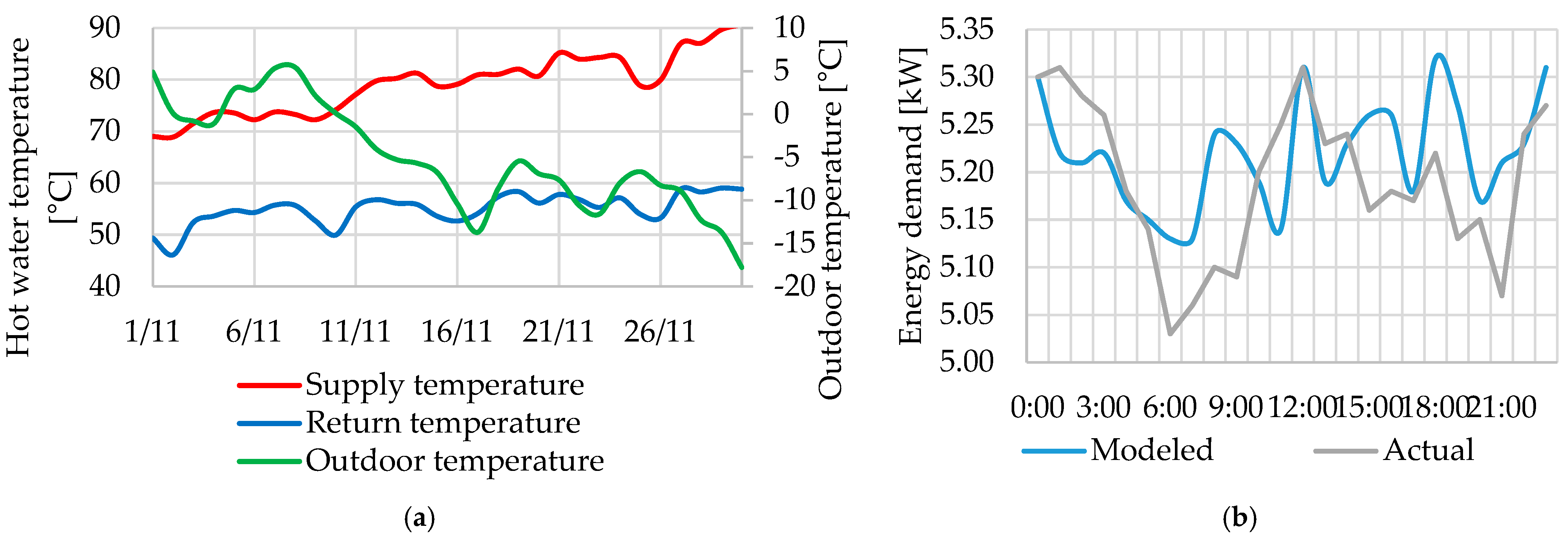
At the same time, supply temperature was still regulated by Equations (2) and (3), leading to overheating and high return temperatures in current conditions (Figure 1).

These results refer to any typical winter day (November, December, January, or February). However, in winter, the supply and return temperatures after and before a substation varied now not only according to the outdoor temperature but also due to wind, solar insolation, and the behavior of occupants changing the adjustment of TRV valves [9].

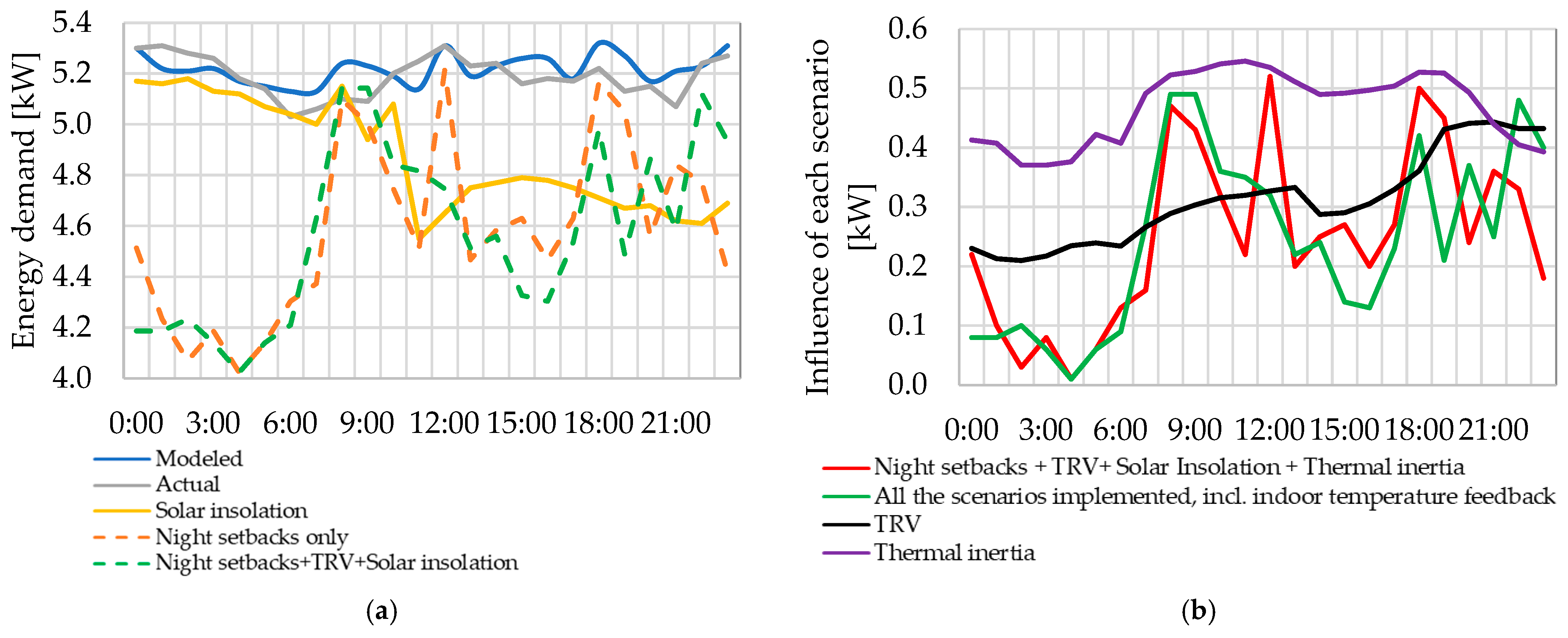
Our methodology suggests a lower profile and more smoothly distributed SH demand, which actually happened in the studied building (Figure 2).

To know the adjusting factors introduced in every simulation, the reader is invited to view

Table 6. A summary of adjusting factors for each scenario.

Scenarios	Number of Radiators with TRVs	Shutdown	Wind	Indoor Temperature Feedback	Occupancy
Notation	ξ	β	μ	Lvent	f
‘As is’	1	1	1	4A	1
#1 (Indoor temperature feedback)	0.7	1	1	4A–10A	0–0.5
#2 (Solar insolation)	0.7	1	1	4A	0–0.5
#3 (Night setbacks)	0.7	1.11	1	4A	0–0.5
#4 (TRVs)	0.5–1	1	1	4A	0–0.5
#5 (Thermal inertia)	0.7	1	1	4A	0–0.5
#6 (Wind)	0.7	1	1–1.15	4A	0–0.5
All the scenarios implemented	0.5–1	1.11	1–1.15	4A–10A	0–0.5

.

In Figure 2, the larger discrepancy in energy demand was localized during the first hours of the day, when the traditional model could not recognize employees’ arrival. A focus on operational data visualized the peak, which was present at noon. After a firmware upgrade, the controller could utilize internal heat gains correctly to decrease energy consumption.

The total daily HVAC heat demand values calculated with the help of a novel methodology and an actual one were 124.6 and 117.1 kWh, respectively. DHW now accounts for less than 14% of daily energy consumption. Total heat demand was also 36% less, which brought a 31% difference compared to the total heat demand calculated according to the traditional methodology. The error decreased since the predicted values differed less from the actual heat demand curve. This was achieved by applying corresponding factors from Equations (5), (11) and (13) to every hour when it was potentially real. Moreover, all of the buildings were now simulated according to the square floor plan and particular details, checking, for instance, whether windows were evenly distributed among the four external walls. That led to more homogenous thermal behavior of the building, which took place in reality across a 24 h period. The difference in total energy demand, especially in DHW heat consumption, was also due to the latest COVID restrictions limiting the number of employees. Being close to the heat demand profile meant the simulation had already become more accurate. This was also relevant since the methodology allowed for cutting the peaks at 8:00 and 21:00 (Figure 2).

Using the correct tools for a simulation enabled utilizing control scenarios when the design indoor temperature was decreased during the night to 16 °C. The same applied when a flexible operation during the day (from 12:00 to 14:00) was implemented, i.e., the setpoint temperature was reduced to 14 °C. From 4:00 to 7:00, energy demand increased because of the gradual increase in DHW consumption and thermal transient processes once the scheduled night setback of the SH system power finished. That resulted in a difference in the total annual SH heat demand of 5–7%. It is worth mentioning that time stamps such as 4:00, 7:00, or 12:00 are provided as benchmarks and indicators only. To ensure coherent and cohesive operation, a setback should begin only when the higher return temperature arrives at the considered substation, and the substation may decrease the heat output due to a lower temperature difference between the return temperature and the required supply temperature [8]. The same but opposite goes to the discharge phase.

Also, considering that the daily average energy supplied to cover the peak was approximately 0.15 kW (Figure 2), it represented a large fraction of the profile, highlighting the influence of the thermal masses. In the case of thermal inertia, the mass flow rate inflowing in an SH system almost does not change when a higher return temperature arrives, as opposed to the other substation scenarios. Instead, excessive heat is dumped into the building envelopes, while temperature waves may pass the pulse onto the return line. Like Luc et al. [5], all the investigated scenarios were based on pre-set schedules.

The abovementioned strategy also decreases DHW heat demand at a substation during non-space heating periods. Tap delay and, associated with that, water consumption on the consumer side (amount to be estimated) can be decreased if a solution with advanced control is used. However, additional heat demand and a high return temperature might occur [9]. Unlike that, Luc et al.’s [5] limitation was that DHW was not included in the modeling. However, the DHW heat demand profile typically has morning and evening peaks, and ignoring them results in inaccuracy during modeling. Another example is clearly visible local peaks induced by individual DHW use and a manual indoor temperature setting through a TRV or air conditioning interface. This led to a lower inconsistency between the actual and optimized load variation curves in relation to an ordinary profile in [25].

As shown in Figure 1b, from 06:00 to 10:00 and from 15:00 to 21:00, the discrepancy between actual and predicted heat consumption was especially large, with a maximum error of 0.15 kW and an average difference of 0.11 kW. The primary reason was that the impact of TRVs and thermal inertia was not considered. For instance, as shown in Figure 2b, the maximum energy demand registered was 0.52 kW at 12:00, while the heat demand at 4:00 was only 0.01 kW. Figure 2a highlights that the heat absorbed due to solar insolation was not negligible, especially when night energy demand (about 5.1 kW) was compared to the total amount consumed by the entire HVAC system during the day (about 4.7 kW, 8.51% less). Because of solar insolation, tuning the control of the building glazing’s transmittance was taking more attention day by day in the literature, and it had already come into use in some buildings, such as high-rise hotel buildings in the United Arab Emirates.

Here, the energy consumption profiles during the daily hours dynamically also changed according to the internal heat gains due to the usage of household appliances (e.g., fridges, kettles, and coffee machines), electronic devices (e.g., desktop computers and all-in-ones), and gadgets (e.g., vending machines or 3D printers). The maximum energy consumption accounted for 0.55 kW at 11:00.

After that, we added three alternative scenarios by engaging the morning and evening setbacks in the control strategy of the DH substation’s valve. The minimum heat consumption and indoor temperature were registered during nighttime hours when the setback was scheduled (from 22:00 to 7:00). Due to this handicap, with the help of TRVs, radiant heating applications could be limited to less occupied or vacant offices. At the same time, employing substation controllers with indoor temperature feedback perfectly integrated the DH technology. It addressed issues like overheating, high thermal load, and slow response time associated with conventional SH systems. Another advantage of flexible operation was energy efficiency. If the indoor temperature feedback was considered, the energy consumption did not reach 0.5 kW in the evening. Moreover, the daily average heat demand decreased, becoming only 0.25 kW. The downside was decreasing the secondary mass flow rate, which may have hampered achieving indoor comfort in the offices where an SH system did not bring ample energy earlier [12].

To compare, Sleptsov et al. [10] investigated an advanced controller (PI one), a combination of the conventional and the previous controller, i.e., a cascaded PI controller consisting of outer and inner loops. The same as [4], we proved that HVAC parameters (such as energy demand and indoor temperature) depend on the number of people (i.e., internal heat gains); therefore, the rational employment of control strategies may contribute to the faster prediction of actual heat demand and indoor thermal comfort in the short term (1–3 h), further guiding the optimal regulation along with the energy saving of HVAC systems.

However, the contribution of some strategies, such as solar insolation, thermal inertia (#5), and wind (#6), was almost negligible (between 1 and 5.1 MWh/day). At the same time, the indoor temperature feedback (#1), night setbacks (#3), and TRVs (#4) brought as much as 18.2% of the total savings (

Table 7. Economic and energy summary.

Scenarios	Cost Saving per Day [EUR]	Energy Saving (kWh)	Energy-Saving Rate [%]
#1 (Indoor temperature feedback)	270.4	38,626	6.4%
#2 (Solar insolation)	24.9	3556	0.6%
#3 (Night setbacks)	347.5	49,647	8.2%
#4 (TRVs)	979.9	21,776	3.6%
#5 (Thermal inertia)	228.5	5078	0.8%
#6 (Wind)	48.6	1080	0.2%
All the scenarios implemented	1899	119.7	19.8%

).

The additional daily effective thermal inertia of the excessive energy dumped into envelopes and furniture elements was 5078 kWh, which brought 1.46 kWh per unit of gross floor surface area. As Johra et al. [13] reported, the additional daily effective thermal inertia of the interior elements was much smaller and ranged from 6.4 to 68 Wh/Km².

The results show that the system saved approximately 49.6 MWh of heat to achieve the quasi-steady-state conditions after the night shutdown. To compare, Guelpa [7] showed that the considered DH system saved about 330 MWh of energy to reach the quasi-steady-state conditions after a night setback. The energy savings of each of the six components ranged between 1080 and 49,647 kWh per day, while the corresponding cost savings were 24.9 and 979.9 EUR as the lower and upper thresholds, respectively.

After adopting the indoor temperature feedback, the average temperature was 21.2 °C with a maximum error of ±1.62 °C. Hence, the methodology may ensure constant thermal comfort and high energy-saving potential. To compare, after Yuan et al. [11] adopted their methodology, they obtained a maximum indoor temperature difference of 0.38 °C and an average error of 0.29 °C.

Here, if the operating parameters were adjusted according to the design indoor temperature of 20 °C all SH season long (from 21 September to 26 April in 2020–2021), the total saving effect in energy demand was 119.7 MWh with the corresponding energy-saving rate of 19.8%. To compare, in [4], the saving effect was achieved at a lower supply temperature, which was highly recommended for an HVAC control system to enhance the physical environment. Indoor comfort was increased by 68% and the energy efficiency by 50%. Yuan et al. [11] concluded that if the operating parameters were adjusted according to the target indoor temperature of 23 °C from November 15 to December 8, the average energy demand would be 37.9 MWh and the associated energy-saving rate was expected to be 5.8 ± 0.1%. Sun et al. [6] reported that the heat demand of all studied substations decreased after implementing a new operational strategy, with energy-saving rates of 5.9%, 6.1%, 6.9%, and 10.0%.

Employing TRV-related savings and considering thermal inertia may ensure a more stable indoor temperature and higher energy performance.

Table 8. The system’s performance was determined after all the scenarios had been implemented. That resulted in a specific annual consumption of 174 kWh/m².

Component	Energy Demand [MWh/Annum]	O&M Costs [kEUR/Annum]
Space Heating	429.4	93.0
DHW	31.1	4.22
AHU Heating	143.3	71.0
Total Base Load & Costs	603.9	168.2

shows that the impact on different components varied greatly, with a total heat demand of 603.9 MWh per year, costs of 168.2 kEUR, and a difference in specific heat consumption of 35.2 kWh/m², which meant less heat demand and a larger cost-saving effect.

Before implementing the new control strategy, the average indoor temperature was 23.5 °C. The heat demand of SH, DHW, and AHU systems ranged between 30 and 430 MWh annually, while corresponding costs were 93.0, 4.22, and 71.0 kEUR, respectively. After implementing all the new control strategies, the average indoor temperature was 20.4 °C with an annual specific heat consumption of 174 kWh/m². To compare, Sun et al. [6] showed the obtained specific energy demand per year as follows: 425 kWh/m², 327 kWh/m², 290 kWh/m², and 281 kWh/m², as shown for each of the four substations.

5. Discussion

First, an opportunity to achieve similar results in the case of any other office building depends on TRVs and whether the building is equipped with an AHU unit or not. As indicated in the literature, when applying a traditional SH system, hot water moves across the building at almost the same temperature no matter what the mass flow rate is. In other words, hot water moves across the entire building from the DH substation to the most remote space, experiencing a limited temperature drop in the supply line. Hence, without TRVs, the entire building tends to overheat. That means the SH system ensures a minimal acceptable indoor temperature in the most remote spaces while other spaces will overheat. Compared with a hydronic SH system, AHU units do not have to heat the entire office. Moreover, they may be turned on only within the occupied zone.

We discussed advancements in experimental and dynamic analyses to evaluate transient effects in building systems, emphasizing the use of detailed models and real-time data to improve accuracy in predicting energy consumption, thermal performance, and occupant comfort. The study showed that night setbacks in HVAC systems could lead to energy savings ranging between 6.4% and 8.2%, as demonstrated in scenarios where SH demand was reduced by 49.7 MWh annually, resulting in 347 EUR/day cost savings. These transient effects, caused by temperature recovery during morning operation, can be analyzed with precision using dynamic simulation tools such as EnergyPlus and TRNSYS.

For this case study, setback periods reduced average indoor temperatures from 23.5 °C to 20.4 °C under controlled conditions, aligning with optimal comfort levels while enhancing efficiency. The scenario when the thermal inertia was considered revealed that high-inertia constructions reduced peak heating or cooling loads by up to 30%, contributing an additional 5078 kWh in annual energy savings and 228 EUR/day in cost reductions.

Similarly, advanced glazing systems with low solar heat gain coefficients can significantly mitigate transient effects. By reducing peak solar gain by as much as 50%, they address up to a 40% variation in internal zone temperatures caused by uneven solar loads, improving occupant comfort by minimizing indoor temperature swings by up to 5 °C during peak solar exposure.

The integration of real-time sensor networks and IoT devices further supports transient analyses. For example, in scenarios where dynamic setpoints were adjusted during unoccupied periods using real-time occupancy detection, energy savings of 10% to 15% were achieved, equivalent to an annual energy reduction of 38.6 MWh with 270 EUR/day in cost savings.

Novel control strategies, which analyze transient behaviors in response to weather changes, demonstrated a 15% improvement in energy efficiency compared to traditional control methods, with optimized HVAC configurations reducing fan energy consumption by 20% during transient periods. Occupant-centric experiments underline the importance of adaptive thermal comfort models, showing that temperature shifts of up to 3 °C can be tolerated without compromising comfort, enabling further energy reductions.

This research emphasizes localized thermal gradients’ impact, particularly under transient conditions, where optimizing façade technologies and shading devices reduced internal temperature swings, enhanced thermal comfort, and improved energy savings. The combination of these strategies yielded a total annual energy saving of 119.8 MWh (19.8%) and cost savings of 1.89 kEUR/day.

These findings illustrate the growing sophistication of dynamic analysis methods and experimental validations, which now capture transient effects of HVAC operations, thermal loads, and material behaviors with remarkable accuracy. This progress is crucial for optimizing energy performance and improving the sustainability of building systems under real-world conditions.

The discussion of the proposed indoor temperature control method results is closely tied to the climatic characteristics of the location, particularly the maximum and minimum outdoor temperatures and the hours of sunlight across different seasons. Using night setbacks in HVAC systems can yield considerable energy savings in regions with extreme winter conditions, where outdoor temperatures frequently drop below freezing. However, the temperature recovery process during morning hours could lead to higher peak loads due to the significant temperature differential between indoor and outdoor conditions. Conversely, the energy savings from setbacks might be smaller in milder climates where outdoor temperatures remain closer to the desired indoor setpoints. Still, the recovery loads are less pronounced, ensuring smoother transitions and enhanced thermal comfort.

The hours of sunlight and seasonal solar gains also play a pivotal role in the performance of indoor temperature control strategies. In climates with high solar insolation during winter, passive solar heating can complement setbacks and reduce the energy required for temperature recovery. On the other hand, in regions with limited sunlight during winter months, setbacks must rely more heavily on the thermal inertia of the building materials to stabilize indoor temperatures without excessive reliance on mechanical heating.

In warmer climates, where the cooling demand is dominant, night setback strategies involve allowing higher indoor temperatures during unoccupied hours, focusing on preventing excessive indoor heat accumulation rather than maintaining low temperatures. In these conditions, integrating advanced glazing systems with low solar heat gain coefficients and shading devices becomes more critical to mitigate solar overheating and ensure occupant comfort.

If this analysis were conducted in a different type of climate, the results and conclusions could differ significantly. For example, in tropical climates with consistently high outdoor temperatures and humidity, the design of temperature control methods would prioritize ventilation and dehumidification rather than heating, and the thermal inertia of building materials would be less relevant compared to insulation and shading strategies. Similarly, in arid climates with large diurnal temperature swings, using thermal mass to capture and release heat would be a priority, and night setback strategies could involve drastic reductions in mechanical cooling during nighttime due to the rapid cooling of outdoor air.

Consequently, the design of buildings must adapt to the specific climatic conditions to optimize energy efficiency and occupant comfort. In cold climates, designs emphasize thermal insulation, airtight construction, and passive solar heating while in hot climates, shading, ventilation, and reflective materials are prioritized. In temperate climates, a balance of these strategies is necessary to address varying seasonal demands. These distinctions highlight the importance of tailoring building design and control methods to the unique challenges and opportunities of different climate types.

The proposed new indoor temperature control method significantly impacts the design of buildings as it requires the careful integration of architectural and mechanical systems to achieve optimal energy efficiency and occupant comfort. Dynamic control strategies, such as night setbacks and indoor temperature feedback, emphasize the need for air conditioning systems that can respond quickly and flexibly to changing conditions. Traditional constant-volume HVAC systems may not be the most suitable option. Instead, variable air volume systems, heat pumps with advanced modulating capabilities, or systems employing model predictive control algorithms, are better suited for such dynamic operations. These systems allow for precise adjustments to airflow and temperature in response to real-time occupancy and climatic variations, ensuring efficient performance.

Alternative layouts for air conditioning systems may also offer advantages. Zoning is particularly important when employing the proposed control method as different spaces within a building can experience varying thermal loads and occupancy patterns. By segmenting the HVAC system into smaller, independently controlled zones, it is possible to apply temperature setbacks selectively, minimizing energy use in unoccupied areas while maintaining comfort in occupied ones. For instance, larger spaces with significant solar exposure may benefit from dedicated systems that can handle peak loads effectively without overburdening other zones.

The distribution of spaces and interior partitions also warrants careful consideration. Open-plan layouts may require additional measures, such as localized temperature controls or thermal barriers, to prevent uneven heating or cooling when applying dynamic temperature adjustments. Conversely, buildings with smaller, compartmentalized spaces might allow for more targeted temperature control, reducing the energy required to condition unoccupied areas. Interior partitions designed with materials that enhance thermal inertia can also help stabilize temperatures during setbacks, complementing the control method by reducing rapid fluctuations and providing passive thermal regulation.

Furthermore, the spatial arrangement should account for the natural flow of heat and air. Spaces with higher heat gains, such as those with significant solar exposure, should be positioned to maximize passive heating benefits in winter or minimize cooling loads in summer. Integrating passive design principles, such as strategically placing windows, shading devices, and ventilation paths, can enhance overall building performance with the proposed control strategy.

Ultimately, the proposed indoor temperature control method necessitates a holistic approach to building design. Integrating advanced, adaptable HVAC systems, flexible layouts, and strategically planned spatial distributions ensures that a building can leverage the benefits of dynamic temperature adjustments while maintaining comfort and minimizing energy consumption.

The proposed indoor temperature control method and associated design strategies can be generalized and applied to various building types and climates to improve energy efficiency and indoor thermal comfort. However, effective implementation requires the careful consideration of several key variables and design criteria. Climate characteristics are crucial in determining how the method can be adapted. The maximum and minimum outdoor temperatures, diurnal temperature swings, solar insolation levels, and seasonal humidity patterns all influence the heating, cooling, and ventilation requirements of a building. For instance, in cold climates with long winters and limited sunlight, the focus would be on maximizing insulation, using thermal inertia to stabilize indoor temperatures, and optimizing passive solar heating strategies. In contrast, in hot and humid climates, strategies prioritize minimizing solar gains, enhancing natural ventilation, and ensuring efficient dehumidification.

The type of building and its operational patterns also affect the applicability of these methods. The control method can rely on scheduled temperature setbacks during unoccupied hours for residential buildings, where occupancy patterns may be predictable and static. In commercial buildings with more variable occupancy patterns, dynamic control methods using real-time data, such as occupancy sensors, become essential. Additionally, the thermal zoning of buildings needs to align with these control methods to allow for localized adjustments, which can reduce energy use without compromising comfort in occupied areas.

Space layouts and material choices are integral to adapting the control method in use. Open-plan spaces require solutions to address uneven temperature distributions, such as localized heating and cooling systems or high-efficiency air circulation strategies. Smaller, compartmentalized spaces may allow for more precise temperature control and energy savings by targeting individual zones. The use of high thermal inertia materials can further enhance the performance of the control method by buffering against temperature fluctuations, which is particularly beneficial in climates with large diurnal swings.

Design criteria that ensure the success of these methods include optimizing building orientation to manage solar exposure, incorporating shading devices and high-performance glazing to control heat gains, and ensuring airtight construction to minimize heat loss or infiltration. These criteria must be adjusted according to the climate type. In cold regions, the emphasis would be on retaining heat and leveraging passive solar gain. In contrast, in hot regions, the focus shifts to shading, ventilation, and reflective materials to minimize cooling loads.

Ultimately, the generalization of this method to other building types and climates requires a context-sensitive approach that integrates climate data, building function, and occupancy behavior. By tailoring the design and operational strategies to these variables, buildings can improve energy efficiency while maintaining or enhancing thermal comfort across diverse climates and use cases.

6. Conclusions

The widespread virus, commonly abbreviated as COVID-19, has led authorities to introduce lockdowns and impose restrictions on the number of employees. That leads to less intensive indoor mixed convection and makes turning off some radiators of an SH system, along with limiting ventilation rates while using the same radiant heating applications, bring the risk of a high return temperature.

There are three site- and building-specific conclusions:

• After implementing new design and operational methods, the overheating of indoor spaces was alleviated. For a particular office building in Omsk (Russia), the average indoor temperature was reduced from 23.5 to 20.4 °C. According to national regulations, the threshold for indoor temperature in an office building during winter in Russia is pretty low and accounts for only 18 °C. Provided that fact, the level of thermal comfort above 20 °C is expressed as ‘normal’.
• The thermal balance between offices is to be enhanced as demonstrated by the indoor temperature, variations in which became less steep. About 19.8% of energy will also be saved during the heating season.
• Regarding the control of the indoor temperature and saving effect, we specifically compared the difference between the maximum values and the minimum values of absolute thermal comfort and heating demand per day, of which the minimum one (0.2%) corresponded to the optimal operation and ensuring the indoor environment by taking the wind into account and the maximum one to night setbacks (8.2%).

The proposed indoor temperature control method employs logged data from sensors and advanced simulations to decrease energy use while maintaining occupant comfort. It integrates model adaptive control strategies for transient effects caused by varying thermal loads, occupancy patterns, and external weather conditions. This approach dynamically adjusts HVAC setpoints based on previous patterns, improving energy efficiency by up to 15% compared to traditional systems.

The new design methods emphasize considering building materials and glazing to minimize temperature fluctuations and delay peak thermal loads. Operational methods prioritize adaptive thermal comfort models, enabling a tolerance of transient temperature variations of up to 3 °C without sacrificing comfort, alongside occupancy-driven setpoint adjustments for periods of low demand, achieving energy savings of 10% to 20%. These innovations enhance building sustainability by harmonizing energy efficiency and thermal comfort in real-world applications.

In a nutshell, the indoor temperature fluctuations became smoother after the new control strategy was implemented. The building energy consumption also decreased drastically. This proves that the control strategy suggested in this paper has considerable heat conservation potential.