Mitigating Long-Term Forecasting Bias in Time-Series Neural Networks via Ensemble of Short-Term Dependencies

Abstract

Time-series forecasting is essential for predicting future trends based on historical data, with significant applications in meteorology, transportation, and finance. However, existing models often exhibit unsatisfactory performance in long-term forecasting scenarios. To address this limitation, we propose the Time-Series Neural Networks via Ensemble of Short-Term Dependencies (TSNN-ESTD). This model leverages iTransformer as the base predictor to simultaneously train short-term and long-term forecasting models. The vanilla iTransformer’s linear decoding layer is optimized by replacing it with an LSTM layer, and an additional long-term model is introduced to enhance stability. The ensemble strategy employs short-term predictions to correct the bias in long-term forecasts. Our extensive experiments demonstrate that TSNN-ESTD reduces the MSE and MAE by 9.17% and 2.3% on five benchmark datasets.

1. Introduction

Time-series data consists of sequences of random variables organized in chronological order, reflecting the changes in a specific entity, phenomenon, or process over time. Examples of time-series data include hourly temperature readings, daily stock closing prices, and monthly sales figures.

Time-series forecasting leverages the inherent patterns within time-series data by establishing an appropriate mathematical model to estimate and predict the values of the series at specific future points or intervals. Recently, time-series forecasting has become an important branch of data science, which aims to find out the inherent regularity by analyzing historical time-series data and then predict the future development trend. It has attracted the attention of both academia and industry in the process of digital and intelligent transformation, especially in meteorology, transportation, finance, and other industries. Diverse time-series models have been developed to deal with weather forecasting, traffic flow prediction, quantitative decision-making, etc.

Recently, numerous scholars have sought to enhance the performance of conventional time-series forecasting models through various techniques like autoregression, recurrent neural networks, Long Short-Term Memory (LSTM), etc. Transformer, as the mainstream technique, was widely introduced by the frontier models, for example, iTransformer, PatchTST, Crossformer, and Autoformer. These transformer-based models significantly improve the ability of multivariate time-series data modeling and achieve state-of the-art performance.

However, the performance is often unsatisfactory when faced with long-term forecasting scenarios. The bias between the predicted value and ground truth is usually within expectation in the short-term scenario but shows an obvious linear growth trend as the forecast period grows. Therefore, improving the awareness and prediction ability of time-series models for long-term scenarios has emerged as a crucial issue.

To facilitate this line of research, we innovatively propose the Time-Series Neural Networks via Ensemble of Short-Term Dependencies (TSNN-ESTD) to fill the gaps of the off-the-shelf model in long-term prediction scenarios. TSNN-ESTD mainly focuses on mitigating the long-term forecasting bias of long-term predictions through hybrid ensemble strategies.

TSNN-ESTD takes iTransformer as the base predictor to train the short-term and long-term prediction models at the same time. Considering the limitations of the linear decoding layer in the vanilla iTransformer, we optimize the decoder layer as the LSTM and additionally train another long-term model for enhancing stability. The short-term prediction results are replicated in multiple copies to ensure the consistency of the output dimension. Then, we design the ensemble strategy that uses the short-term prediction results to correct the prediction bias of the long-term model. In this situation, TSNN-ESTD enhances the iTransformer by substituting its linear decoding layer with an LSTM layer and incorporating an additional long-term forecasting model to ensure stability. A hybrid ensemble method is employed to integrate short-term and long-term predictions, thereby mitigating bias in long-term forecasts.

The main contributions of this paper can be summarized as follows:

(1)

We investigate the efficacy of numerous existing methodologies in both short-term and long-term forecasting and construct a general ensemble learning framework for multivariate time-series forecasting.

(2)

We optimize the decoding layer structure of iTransformer by modifying the MLP to an LSTM layer to improve the ability of long-term dependencies.

(3)

We explore the ensemble strategy of multiple base predictors with different scales to mitigate the long-term forecasting bias in time-series neural networks with short-term dependencies.

(4)

Extensive experiments have been conducted to demonstrate the superiority of our proposal.

2. Related Work

2.1. Time-Series Forecasting with Statistic Theory

Statistical methods serve as the origin and foundation of time-series prediction, utilizing mathematical modeling techniques to model and analyze the trends, periodicity, and randomness within data. Early statistical methods include Moving Average (MA) and simple exponential smoothing (ES), which predict future trends by smoothing data in a weighted average or exponentially weighted manner [1,2].

Subsequently, the Autoregressive (AR) and Moving Average (MA) models were integrated to develop the Autoregressive Moving Average (ARMA) model [3], which can effectively capture the auto-correlation and average characteristics of time series by combining the characteristics of Autoregressive and Moving Averages. To deal with non-stationary time series, the Autoregressive Integrated Moving Average (ARIMA) [4] model is proposed to transform non-stationary series into stationary series by difference operation, to improve the prediction accuracy.

In addition, Holt [5] introduced the exponential smoothing method, which demonstrates excellent performance in modeling time series with trend and seasonality. Ralaivola [6] extended this work by developing the state space model and the local linear trend model, enhancing the adaptability of models to dynamic changes in real-world data. Hamilton [7] made groundbreaking contributions to nonlinear state transition modeling, enabling the capture of mutational events in time series. Hyndman [8] further advanced the field by introducing the ETS framework, which facilitates automatic model structure selection and significantly improves the generalization capability of forecasting models.

These methods perform well under small-scale data and strong assumptions, which effectively enhances seasonality, trend, and periodicity. However, with the expansion of data scale and the complexity of the data generation mechanism, traditional statistical methods face bottlenecks in high-dimensional multivariate, nonlinear, and long-term dependence modeling, lacking sufficient expressive power and making it difficult to capture complex dynamic patterns. Aiming at this problem, this paper proposes an ensemble strategy that exploits short-term dependence to mitigate long-term prediction bias.

2.2. Time-Series Forecasting with Machine Learning

With the improvement of computing power and the convenience of data acquisition, traditional machine learning models have been introduced into time-series prediction. These models can achieve accurate prediction of time-series data by learning the complex mapping relationship between input features and output targets without explicit modeling [9,10,11].

Zhang [12] introduced multi-layer perceptron (MLP) into time-series prediction and applied the nonlinear mapping function through the backpropagation algorithm for nonlinear dynamic systems. Cao [13] proposed the Support Vector Regression (SVR) time-series model, which adopted the ε-insensitive loss function and kernel technique to have a stronger generalization ability for nonlinear data. Lemke [14] applied XGBoost to financial market prediction and selected the closing price and trading volume lagging periods as key factors through feature importance analysis, which verified the adaptability of the gradient boosting tree to non-stationary time series. Taieb [15] proposed a combined regression framework (CRF), which decomposed multi-step prediction into several independent regression problems and introduced the bagging strategy to reduce variance. Bontempi [16] proposed a Lazy Learning framework, which dynamically constructs neighbor sub-models through local weighted regression, and realizes stable prediction when the feature dimension is extended to 50 dimensions on UCI multivariate datasets, thus solving the problem of dimension disaster of high-dimensional time series.

Recent studies show that linear models are still competitive in high-signal-to-noise-ratio time-series data. Zeng [17] used learnable linear layers instead of complex nonlinear transformations and restricted the Frobenius norm of the weight matrix through ridge regression, which achieved the same accuracy as Autoformer with only a few parameters on the ETTh1 dataset. Li [18] employed a linear transformation approach for time-series forecasting, demonstrating that simple linear models can effectively capture complex temporal patterns. Zhou [19] further designed a deep linear network to achieve multi-scale trend decomposition by stacking multiple linear layers, which achieved performance comparable to complex models at low complexity.

Meanwhile, researchers have proposed a variety of alternative deep learning architectures. For example, Festag [20] constructed a dual recurrent architecture based on GAN, in which both the generator and the discriminator were designed to capture the dynamic characteristics of time series. Staffini [21] employed a Deep Convolutional Generative Adversarial Network (DCGAN) that utilizes multi-channel convolution to extract features from stock data and generate future price series. Oreshkin [22] proposed the Neural Basis Expansion Analysis (N-BEATS) architecture, which focuses on mining the intrinsic interpretable structure of time series. Bai [23] introduced causal convolution, extended convolution, and parallel computing to solve the problem of slow training speed and difficulty in capturing long-term dependence of RNN series in sequence modeling, and improved the performance of sequence prediction tasks. Xiang [24] integrated multivariate feature extraction, spatiotemporal decomposition, and LSTM memory units. This approach effectively combines the spatial features extracted by SATCN with the temporal features derived from LSTM, allowing the model to comprehensively account for both spatial and temporal dimensional information. Cheng [25], inspired by TCN, proposed a new basic structure for temporal convolution that combines ds-inception and 1D CBAM mechanisms.

Machine learning methods break the strict assumptions on data distribution and demonstrate significant capability in complicated scenarios. However, most models tend to focus on the local information of the current time step, which makes it difficult to capture the deep temporal dependencies in the sequence. To solve this problem, researchers have begun to introduce the attention mechanism into time-series prediction, which promotes the wide application of the transformer structure.

2.3. Time-Series Forecasting with Transformer Structure

Recently, transformer architectures have made tremendous progress in the field of natural language processing, which has become a new mainstream research paradigm. Considering the similar characteristics of time-series data and text data in the sequential relationship, many scholars have introduced the transformer structure to leverage the time-series forecasting methods with diverse optimized recurrent neural networks [26,27].

Liu [28] considered each variable as an independent variates token and constructed the iTransformer model with the multi-head self-attention mechanism, thus effectively capturing the complex collaborative relationship between variables in multivariate time series and improving the modeling ability of multivariate information. Borrowing the idea of patch embedding in image processing, Nie [29] divided the time series into patches of fixed length and proposed the PatchTST model, which better extracts global dependencies while preserving local features and effectively alleviates the problem of capturing long-distance dependencies in the time dimension. Zhang [30] proposed Crossformer, which constructs a dual-channel attention mechanism, namely the time channel and variable channel, to adaptively learn the cross-dependencies between time points and variables. The ability to model the interaction between variables is enhanced. Das [31] developed a time-series modeling method called TiDE, which decomposes the series into trend and seasonal components and models them separately using the attention mechanism. It significantly improves the stability and accuracy of the model in long-term prediction scenarios. Wu [32] innovatively introduced 2D temporal modeling structures that not only model the temporal dimension of time series but also introduce 2D convolution operations across time periods, thus capturing complex nonlinear temporal evolution patterns. Liu [33] proposed SCINet, using a learnable Sample Convolution Interaction module. This structure allows the model to learn the nonlinear interaction between different time steps and performs efficient time modeling by layer-by-layer convolution. Zhou [34] enhances the transformer model by incorporating frequency decomposition. The time series is projected into the frequency domain, and then the frequency components are modeled by self-attention, which allows the model to capture both short-term and long-term dependencies in time-series data. Liu [35] introduced a stationarity enhancement module to make the dynamic characteristics of time series more stationary through an adaptive transformation mechanism, aiming at the difficulty of modeling non-stationary time series. Wu [36] introduced the auto-correlation mechanism to mine the periodicity and trend in time series. This method achieved leading performance in multiple prediction tasks through stacked decomposition modules and reconstruction mechanisms.

The transformer structure utilizes the attention mechanism to capture the potential correlation of dynamic time series and then makes predictions for the next time steps, instead of the conventional recurrent neural network structure. However, the model exhibits limited capacity for long-term dependency capture and is unable to provide accurate predictions over extended periods.

To address this limitation, the proposed TSNN-ESTD utilizes a short-term predictor based on iTransformer, optimistically strengthens long-term modeling, and introduces a bias-correction strategy that combines short-term outputs to calibrate long-term predictions. This design improves stability, reduces cumulative error, and significantly alleviates prediction bias in long-term scenarios.

3. Methodology

The multivariate time-series data can be formalized as $X=\left\{X_1,X_2,\dots ,X_T\right\}\in {\mathbb{R}}^{T\times N}$. Each element $X_i$ represents the value of $N$ variables at timestamp $i$. In addition, the constants T and N denote the dimension of time steps and variates, respectively. Time-series forecasting intends to analyze the latent relationship of the observation and then predict the next L time steps, i.e., $Y=\left\{X_{T+1},X_{T+2},\dots ,X_{T+L}\right\}\in {\mathbb{R}}^{L\times N}$. TSNN-ESTD focuses on improving the long-term dependence capture ability of traditional time-series prediction models, so as to optimize the long-term prediction performance.

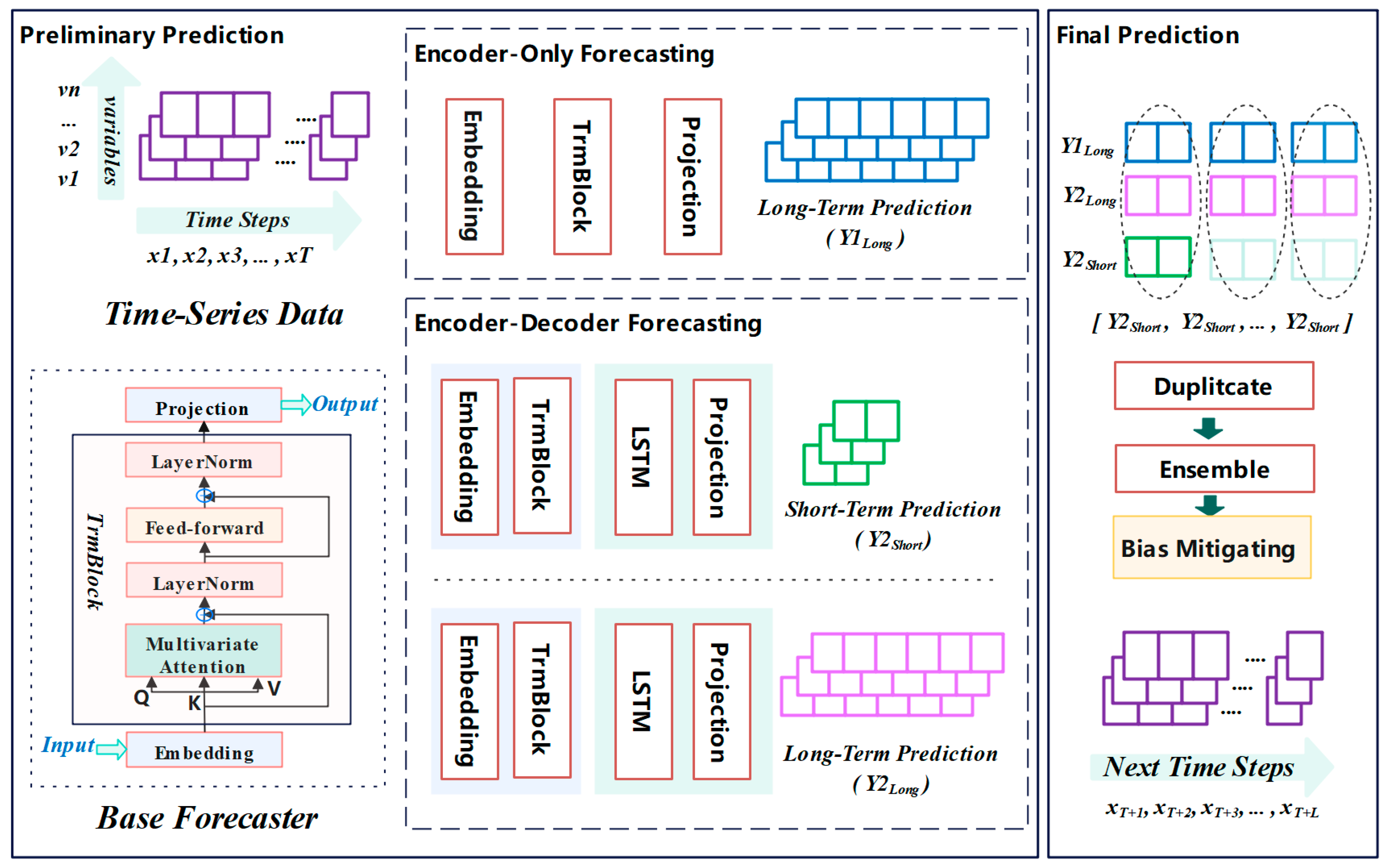
As shown in Figure 1, the two-stage integration strategy was adopted to correct the deviation of long-term prediction with the help of short-term prediction. First, the vanilla encoder-only forecaster iTransformer was utilized to achieve the preliminary prediction. Furthermore, we introduced the encoder–decoder architecture to optimize the original version for both short-term and long-term prediction. Subsequently, we explored the ensemble strategy of the three benchmark predictors to obtain the final prediction.

Figure 1. TSNN-ESTD framework. (Left part: Base time-series forecaster network structure. Middle part: Three individual time-series forecasters with encoder-only and encoder–decoder architecture. Right part: Ensemble strategy for bias mitigating).

TSNN-ESTD retains the iTransformer encoder (which uses self-attention and inverted embeddings to capture global dependencies) and replaces the MLP projection in the decoder with an LSTM-based decoder. The LSTM decoder complements the iTransformer encoder by addressing the MLP’s inability to model sequential dependencies during generation, ensuring coherent and stable predictions while leveraging the encoder’s global insights. This hybrid approach balances global context and local temporal coherence, particularly beneficial for complex time-series forecasting tasks.

3.1. Encoder-Only Forecasting

TSNN-ESTD takes the advantages of diverse time-series forecasters into consideration and integrates both encoder-only and encoder–decoder architectures. The encoder-only forecaster is consistent with the iTransformer. Instead of aggregating different variables with the same timestamp, all variables with different time steps are regarded as the independent input tokens $h_i^0$ in the embedding procedure. Specifically, the embedding layer establishes the mapping from ${\mathbb{R}}^{\mathrm{T}}$ to ${\mathbb{R}}^{\mathrm{D}}$, where $\left\{X_{1i},X_{2i},\dots ,X_{Ti}\right\}, i\in [1,N]$ denotes the values of the i-th variable with different timestamps. Subsequently, the tokens of a sequence of the i-th variables are computed as the input layer in Equations (1) and (2).

$$h_i^0=Embedding(X_{1i},X_{2i},\dots , X_{Ti})$$

(1)

$$H=\left\{h_1,h_2,\dots ,h_N\right\}\in {\mathbb{R}}^{\mathrm{N}\times \mathrm{D}}$$

(2)

In addition, the acquired variate tokens engage in interactions through self-attention mechanisms and are processed independently by the shared feed-forward network within each TrmBlock, as shown in Equation (3). The structure of TrmBlock is consistent with that of the classic Transformer [28].

$$H^{l+1}=TrmBlock\left(H^l\right)$$

(3)

Afterward, the multi-layer perceptron (MLP) as the projection layer is conducted to align the high-level embedding $H\in {\mathbb{R}}^{N\times D}$ to the prediction $H\in {\mathbb{R}}^{N\times L}$, i.e., the value of N variable at future $L$ time steps. Notable, multivariate time-series data for long time steps are forecasted in a straightforward manner, which is formalized as $Y{1}_{Long}\in {\mathbb{R}}^{\mathrm{N}\times \mathrm{L}}$ in Equation (4).

$$Y{1}_{Long}=Projection\left(H^{l+1}\right)$$

(4)

The encoder-only model is trained independently with the mean squared error (MSE) loss function, which quantifies the discrepancy between the predicted values and the ground truth, as illustrated in Equation (5). Here, $N_L$ represents the number of samples, $Y_i$ denotes the ground truth for the i-th sample, and $Y{1}_{Lon{g}_i}$ is the final forecast value for the i-th sample.

$${Loss}_1={\displaystyle \frac{1}{N_L}}{\sum }_{i=1}^{N_L}{\left(Y_i-Y{1}_{Lon{g}_i}\right)}^2$$

(5)

3.2. Encoder–Decoder Forecasting

The encoder-only forecasting architecture is easier to implement with a lower computation complexity. This schema focuses on capturing the potential links between variables at the time steps before and after. The projection layer simply takes the basic MLP mapping the higher-order representation to the desired output dimension. Considering that MLPs process each time step independently, lacking mechanisms to model temporal relationships between predicted steps, it is problematic for autoregressive decoding, where each prediction depends on prior outputs. On the other side, MLPs cannot maintain a hidden state across predictions, making it difficult to enforce coherence in multi-step forecasts (e.g., trend continuity or seasonality alignment). To deal with this issue, the decoder layer is introduced to describe the sequence relation of time-series data better based on the idea of auto-encoder.

Similarly, the encoder layer contains two components of the embedding and TrmBlock layer, which is consistent with the encoder-only framework. The embedding layer converts the observed time-series data input into a number of tokens for each variable characteristic in Equation (6). Then, the variate token is fed into the transformer components to learn the high-order representation as shown in Equation (7).

$$H^0:,n=Embedding\left(X:,n\right)$$

(6)

$$H^l=Transformer\left(H^{l-1}\right)$$

(7)

Afterward, we utilize the Long Short-Term Memory (LSTM) as the decoder layer to achieve the complex relationship between the elements and the time evolution law as shown in Equations (8)–(10), where $I_t,F_t,Q_t$ denote the input, forget, and output gates. These equations show how the current input $X_t$ and the previous hidden state $H_{t-1}$ are transformed with weight matrices W and bias vectors b. Afterwards, the sigmoid activation function σ is utilized for maping the input to an interval of (0, 1). LSTM explicitly models sequential dependencies between predictions, using their recurrent structure to iteratively update the hidden state. Meanwhile, LSTM is more stable than ordinary RNN because its gating mechanism can effectively capture long-term dependence and alleviate the gradient vanishing and explosion problem.

$$I_t=\sigma \left(X_t{W}_{xi}+H_{t-1}{W}_{hi}+b_i\right)$$

(8)

$$F_t=\sigma \left(X_t{W}_{xf}+H_{t-1}{W}_{hf}+b_f\right)$$

(9)

$$O_t=\sigma \left(X_t{W}_{xo}+H_{t-1}{W}_{ho}+b_o\right)$$

(10)

In addition, the candidate memory denoted by $C_t$ is calculated by Equations (11) and (12), where $\widetilde{C_t}$ denotes the candidate cell state, and tanh denotes the hyperbolic tangent activation function. The operator symbol ⊙ represents element-wise multiplication (Hadamard product). In addition, $W_{xc}$ and $W_{hc}$ denote the weight matrix of the candidate cell state, which is used to linearly transform the concatenation vector of the hidden state at the previous time and the input at the current time, and $b_c$ represents the bias term of the candidate cell state.

$$\widetilde{C_t}=tanh(X_t{W}_{xc}+H_{t-1}{W}_{hc}+b_c)$$

(11)

$${\mathrm{C}}_{\mathrm{t}}=F_t\odot C_{t-1}+I_t\odot \widetilde{C_t}$$

(12)

The forget gate is used to control the memory state of the previous step, and the input gate controls the candidate memory state, as shown in Equation (13).

$$H_t=O_t\odot tanh\left(C_t\right)$$

(13)

Also, the MLP is used to align the decoder results to the desired output $Y{2}_{Long}\in {\mathbb{R}}^{\mathrm{N}\times \mathrm{L}}$, as shown in Equation (15).

$$Y{2}_{Long}=ML{P}_{Long}\left({\mathrm{H}}_{\mathrm{t}}^{l+1}\right)$$

(14)

Afterward, the model is trained independently by minimizing the mean squared error (MSE), which calculates the average squared difference between the predicted values and the target values as shown in Equation (15).

$${Loss}_2={\displaystyle \frac{1}{N_L}}{\sum }_{i=1}^{N_L}{\left(Y_i-Y{2}_{Lon{g}_i}\right)}^2$$

(15)

3.3. Long-Term Bias Mitigating

Considering the pitfall of long-term prediction, we additionally forecast the short term as preparation for correcting the bias of the long-term prediction. Specifically, this only requires adjusting the parameters of the final MLP layer in the encoder–decoder framework to obtain the short-term prediction $Y{2}_{short}\in {\mathbb{R}}^{\mathrm{N}\times \mathrm{S}}$ as Equations (16) and (17), where $S$ is less than and divisible by $L$. In other words, L can be written as $n\times S$, where n is an integer.

$$\begin{gathered} Y{2}_{Short}=ML{P}_{Short}\left({\mathrm{H}}_{\mathrm{t}}^{l+1}\right) \\ L=n\times S, n,L,S\in {\mathbb{Z}}^{+} \end{gathered}$$

(16)

Meanwhile, the loss function is defined as the mean squared error (MSE) for independent training as shown in Equation (17), where $N_s$ represents the number of samples.

$${Loss}_3={\displaystyle \frac{1}{N_s}}{\sum }_{i=1}^{N_s}{\left(Y_i-Y{2}_{shor{t}_i}\right)}^2$$

(17)

In this situation, the preliminary long-term forecast $Y{1}_{Long}\in {\mathbb{R}}^{\mathrm{N}\times \mathrm{L}}$ from the encoder-only framework and both the long-term $Y{2}_{Long}\in {\mathbb{R}}^{\mathrm{N}\times \mathrm{L}}$ and short-term $Y{2}_{Short}\in {\mathbb{R}}^{\mathrm{N}\times \mathrm{S}}$ forecast from the encoder–decoder framework are available for subsequent bias mitigating and final forecasting. To align the dimension, the extended sequence is constructed by replicating the short-time prediction sequence into n copies as shown in Equation (18). In most conditions, time-series data such as temperature and electricity do not fluctuate much and inherently show a strong periodic law. Therefore, iterating short-term forecasting is not just an error correction trick but a mechanism to decompose long-term dependencies into locally coherent segments. By averaging these segments, the model constructs a long-term forecast that reflects the hierarchical, multi-scale nature of real-world time-series data. This approach effectively bridges the gap between the global insights provided by the transformer encoder and the decoder’s requirement for local temporal fidelity, ultimately enhancing dependency modeling and mitigating error propagation.

$$\mathrm{Y}{2}_{\mathrm{s}\mathrm{h}\mathrm{o}\mathrm{r}\mathrm{t}}^{rep}=[Y{2}_{Short},Y{2}_{Short},\dots ,Y{2}_{Short}]$$

(18)

Furthermore, TSNN-ESTD integrates these three outputs by means of a weighted average and gives the final forecast as shown in Equation (19). The core contribution of TSNN-ESTD is to correct the bias of long-term forecasts with short-term forecasts. According to our preliminary experiments, it is found that the model generally achieves the best performance when the weights of the two long-term models are adjusted to be the same. The long-term predictions of both models with encoder-only and encoder–decoder architectures are treated as equally important. The final result is then calculated by the weighted average of the long-term and short-term forecast series.

$$\begin{gathered} Y_{Final}=\alpha \times {\displaystyle \frac{1}{2}}(Y{1}_{Long}+Y{2}_{Long})+\mathsf{\beta }\times \mathrm{Y}{2}_{\mathrm{s}\mathrm{h}\mathrm{o}\mathrm{r}\mathrm{t}}^{rep} \\ s.t \alpha +\beta =1 \end{gathered}$$

(19)

At this point, the long-term forecasts $Y{1}_{Long}$ and $Y{2}_{Long}$ at time steps 1 to S, S + 1 to 2S, and so on, can be corrected by the short-term forecast $Y{2}_{Short}$, which can help the model’s performance in capturing long-term dependencies to some extent.

4. Experiments Analysis and Discussion

4.1. Data Statistic

TSNN-ESTD is committed to breaking the bottleneck of the time-series model in long-term prediction. For evaluation, we test the performance on the benchmark dataset as shown in Table 1.

Table 1. Data statistics.

Dataset	Variates	Time Steps	Granularity
ECL	321	26,305	1 h
Exchange	8	7588	1 day
Traffic	862	17,544	1 h
Weather	21	52,696	10 min
ETT	7	17,420/69,680	1 h/15 min
ERA5	38	17,544	1 h

ECL collects the electricity consumption of 321 clients. Exchange is a financial dataset including the daily exchange rates for eight countries from 1990 to 2016. Traffic describes road occupancy and contains hourly data recorded by sensors on San Francisco highways. Weather consists of 21 meteorological indicators, including air temperature and humidity, which are recorded every 10 min. In addition, ETT is a composite transformer temperature dataset consisting of two 1-hour-level (ETTh) and two 15 min level datasets (ETTm) with seven oil and power transformer load features. Furthermore, we conduct experiments on the additional real industry data ERA5, which is the temperature and wind speed of 3850 automatic stations at 1 h intervals over a period of 2 years, provided by our partner.

4.2. Comparison with Other Frontier Methods

TSNN-ESTD utilizes the short-term forecast to mitigate the long-term forecast with the ensemble strategy, which enriches the capability of long-term dependency capturing. Table 2 and Table 3 demonstrates the performance of TSNN-ESTD and other frontier methods on four benchmark datasets and one composite dataset. The prediction time step is set to 96 with reference to the current literature.

Table 2. Performance on four benchmark datasets.

	ECL		Exchange		Traffic		Weather
	MSE	MAE	MSE	MAE	MSE	MAE	MSE	MAE
iTransformer [28]	0.148	0.240	0.086	0.206	0.395	0.268	0.174	0.214
Rlinear [18]	0.201	0.281	0.093	0.217	0.649	0.389	0.192	0.232
Dlinear [19]	0.197	0.282	0.088	0.218	0.650	0.396	0.196	0.255
PatchTST [29]	0.181	0.270	0.088	0.205	0.462	0.295	0.177	0.218
Crossformer [30]	0.219	0.314	0.256	0.367	0.522	0.290	0.158	0.230
TiDE [31]	0.237	0.329	0.094	0.218	0.805	0.493	0.202	0.261
TimesNet [32]	0.168	0.272	0.107	0.234	0.593	0.321	0.172	0.220
SCINet [33]	0.247	0.345	0.267	0.396	0.788	0.499	0.221	0.306
FEDformer [34]	0.193	0.308	0.148	0.278	0.587	0.366	0.217	0.296
Stationary [35]	0.169	0.273	0.111	0.237	0.612	0.338	0.173	0.223
Autoformer [36]	0.201	0.317	0.197	0.323	0.613	0.388	0.266	0.336
TSNN-ESTD	0.133	0.225	0.046	0.152	0.585	0.427	0.129	0.151

Table 3. Performance on one composite dataset.

	ETTm1		ETTm2		ETTh1		ETTh2		Average
	MSE	MAE	MSE	MAE	MSE	MAE	MSE	MAE	MSE	MAE
iTransformer [28]	0.334	0.368	0.180	0.264	0.386	0.405	0.297	0.349	0.299	0.347
Rlinear [18]	0.355	0.376	0.182	0.265	0.386	0.395	0.288	0.338	0.303	0.344
Dlinear [19]	0.345	0.372	0.193	0.292	0.386	0.400	0.333	0.387	0.314	0.363
PatchTST [29]	0.329	0.367	0.175	0.259	0.414	0.419	0.302	0.348	0.305	0.348
Crossformer [30]	0.404	0.426	0.287	0.366	0.423	0.448	0.745	0.584	0.465	0.456
TiDE [31]	0.364	0.387	0.207	0.305	0.479	0.464	0.400	0.440	0.363	0.399
TimesNet [32]	0.338	0.375	0.187	0.267	0.384	0.402	0.340	0.374	0.312	0.355
SCINet [33]	0.418	0.438	0.286	0.377	0.654	0.599	0.707	0.621	0.516	0.509
FEDformer [34]	0.379	0.419	0.203	0.287	0.376	0.419	0.358	0.397	0.329	0.381
Stationary [35]	0.386	0.398	0.192	0.274	0.513	0.491	0.476	0.458	0.392	0.405
Autoformer [36]	0.505	0.475	0.255	0.339	0.449	0.459	0.346	0.388	0.389	0.415
TSNN-ESTD	0.305	0.360	0.221	0.307	0.380	0.395	0.144	0.251	0.262	0.328

Rlinear [18] employs a linear transformation approach for time-series forecasting, demonstrating that simple linear models can effectively capture complex temporal patterns. Dlinear [19] employs a deep linear model for time-series forecasting, demonstrating that deep linear architectures can effectively capture temporal patterns. iTransformer reimagines transformer architecture for time-series forecasting by embedding each time series as variate tokens, enabling the capture of multivariate correlations through self-attention mechanisms. PatchTST [29] treats time-series data as sequences of patches, similar to image processing, allowing the transformer to model long-term dependencies effectively. Crossformer [30] introduces a cross-dimensional attention mechanism to capture both temporal and inter-variable dependencies in multivariate time-series forecasting. TiDE [31] focuses on modeling temporal dynamics by decomposing time series into trend and seasonal components, enhancing forecasting accuracy. TimesNet [32] utilizes a temporal 2D-variation modeling approach to capture complex temporal patterns in time-series data. SCINet [33] introduces a sample convolutional interaction network to model complex temporal dynamics in time-series forecasting. FEDformer [34] enhances transformer models by incorporating frequency decomposition, allowing the model to capture both short-term and long-term dependencies in time-series data. Stationary [35] focuses on modeling non-stationary time-series data by introducing a stationarity assumption, improving forecasting performance. Autoformer [36] introduces an auto-correlation mechanism to transformer models, enabling the capture of both trend and seasonal components in time-series forecasting.

Compared with conventional individual MLP-based and transformer-based models, TSNN-ESTD achieves relatively lower forecast error in the metric of mean squared error (MSE) and mean absolute error (MAE) in most situations with the long-term bias mitigating trick. Furthermore, TSNN-ESTD additionally introduces the encoder–decoder forecaster on the basis of the encoder-only iTransformer model. The mean squared error has been reduced by 10.14%, 46.51%, and 25.86% on dataset ECL, Exchange, and Weather datasets, respectively, where the relative error is calculated as the quotient of the reduced error and the original error. However, the traffic data does not have such a strong periodic law, so the short-term deviation prediction correction effect designed by TSNN-ESTD is not so significant. Meanwhile, TSNN-ESTD reduces the MSE and MAE by 12.4% and 5.4%, respectively, on the four composite temperature datasets of ETTm1, ETTm2, ETTh1, and ETTh2. In summary, there was a reduction in MSE and MAE by 9.17% and 2.3% on the five benchmark datasets.

4.3. Performance of Long-Term Forecasting

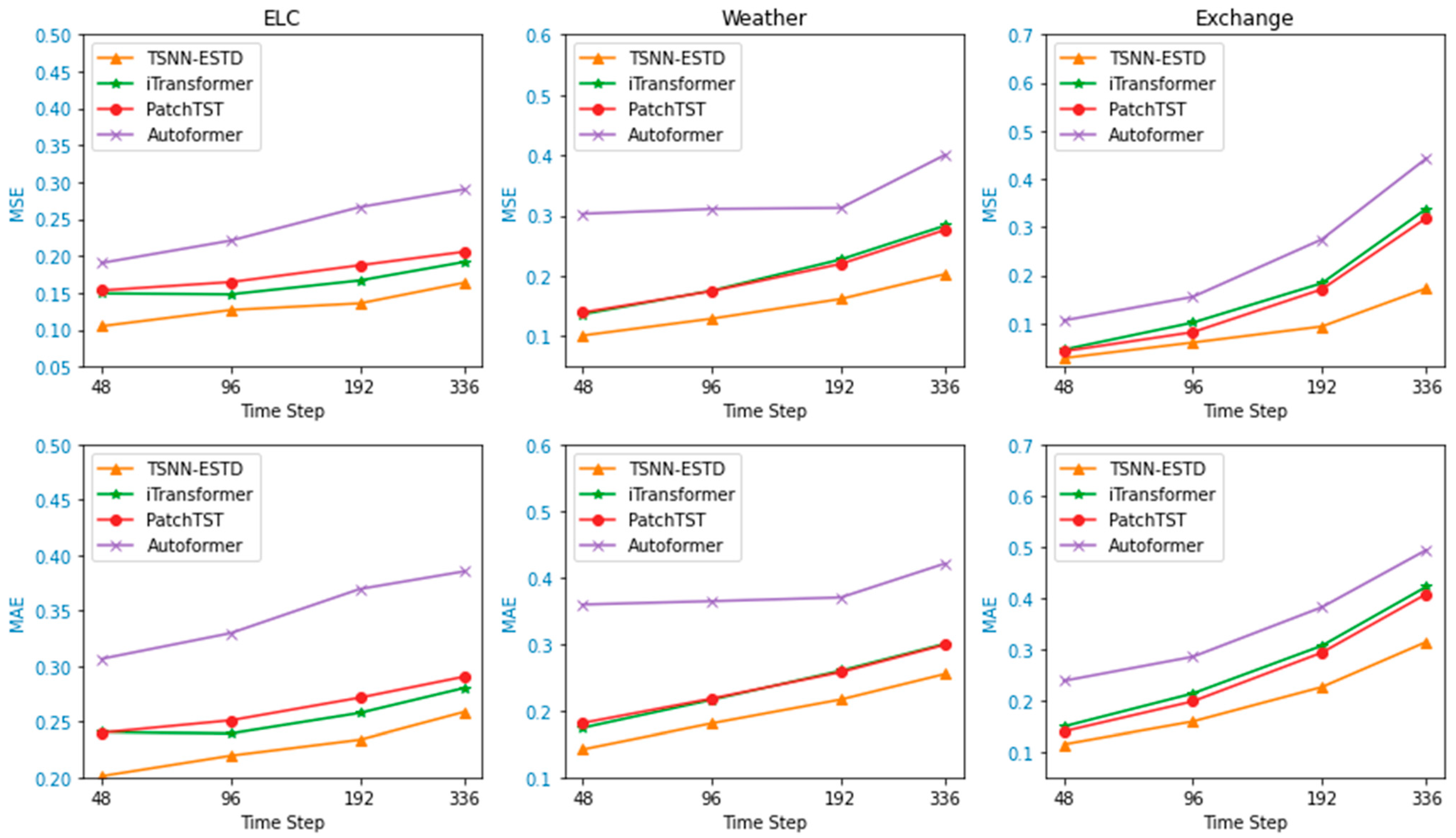
TSNN-ESTD applies an integrated strategy and strives to use short-term dependencies to correct long-term bias. Figure 2 further discusses the performance under different prediction step sizes. In detail, we verify the MAE and MSE metric of TSNN-ESTD and three mainstream frontier models (iTransformer, PathchTST, and Autoformer) under 48 to 336 time steps. Since PathchTST and Autoformer are inherently encoder–decoder architectures, we only integrate the short term and long term in the hope of reducing the long-term prediction bias.

Figure 2. Performance of long-term forecasting.

For short-term forecasting, there is little difference between the prediction errors of these models. Compared with the other approaches, TSNN-ESTD explores short-term dependence to bias the growth period, and the prediction error is relatively low. As the time step lengthens, the prediction errors of all models show a gradually increasing trend. However, the curve of TSNN-ESTD is more gentle, which also proves the superiority of the model in long-term prediction.

4.4. Effectiveness of Long-Term Bias Mitigating

TSNN-ESTD takes iTransformer as the baseline model for constructing the ensemble model with long-term and short-term forecasting strategies. Therefore, this represents a universal optimization approach that is also applicable to various types of time-series models. Figure 3 shows the performance of the original version and bias mitigation of three different models. When the forecasting time step is set as 96, the MSE metric of Autoformer, PatchTST, and iTransformer is reduced by 24.7%, 28.4%, and 27.2%, respectively. In addition, the prediction error is further reduced by 33.3%, 30.4%, 30.6% with 336 time steps. This indicates that our approach serves as a universal bias-correction strategy, demonstrating effectiveness across various models, with particularly significant improvements observed in long-term predictions.

Figure 3. Performance of long–term bias mitigating.

4.5. Impact of Different Parameter $S$

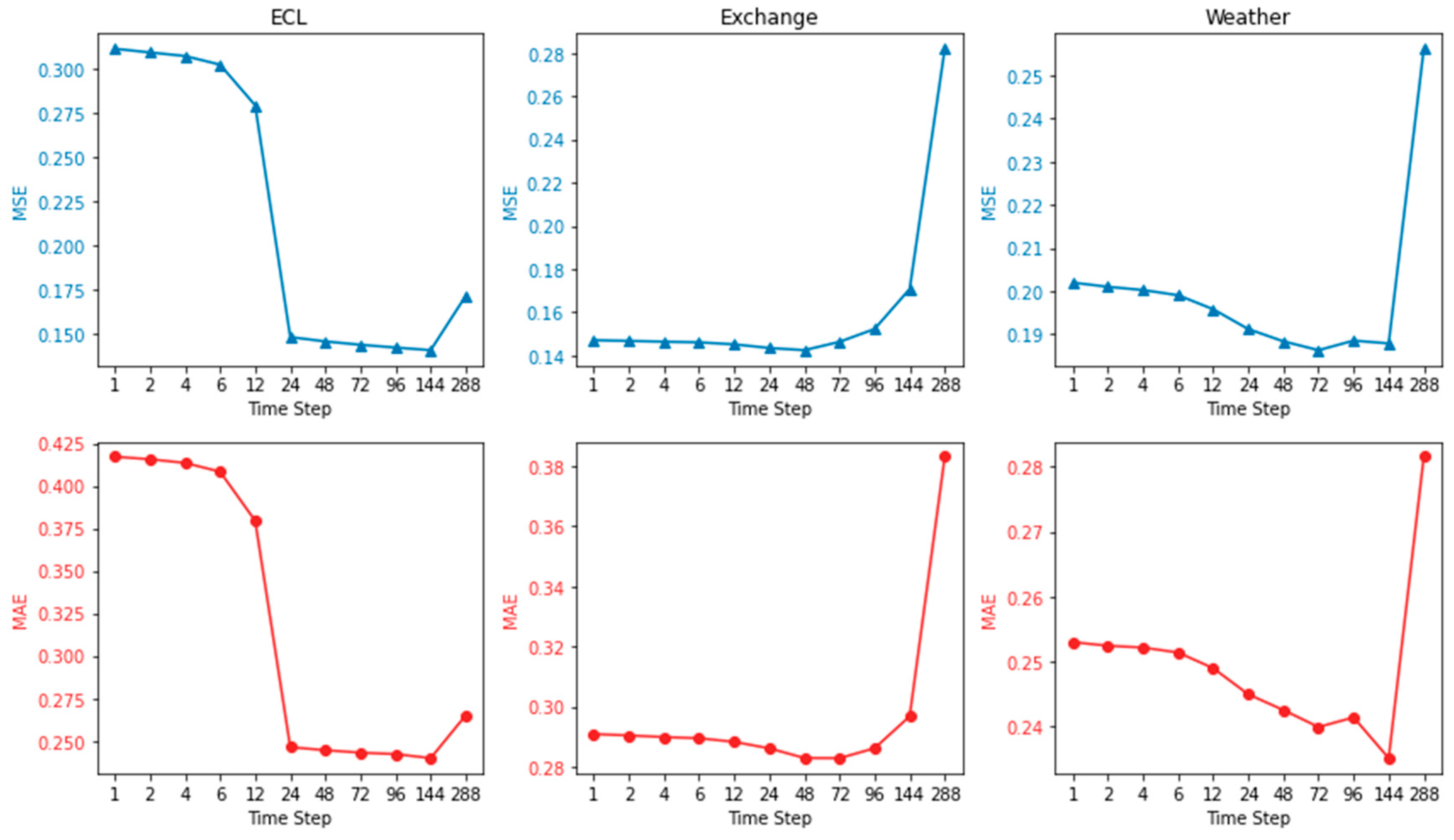
TSNN-ESTD fuses the results of long-term prediction ($Y{1}_{Long}\in {\mathbb{R}}^{\mathrm{N}\times \mathrm{L}},Y{2}_{Long}\in {\mathbb{R}}^{\mathrm{N}\times \mathrm{L}}$) and short-term $(Y{2}_{short}\in {\mathbb{R}}^{\mathrm{N}\times \mathrm{S}}, L=n\times S)$ prediction by the strategy of weighted average. This section addresses the problem of choosing the time step $S$ for short-term prediction. Specifically, we fixed the input time step as 96 and the long-term prediction time step as 288, and, on this basis, integrated the results of the short-term forecast with different time steps from 1 to 288, as shown in Figure 4. The TSNN-ESTD model makes multiple copies of the results of the short-term predictions to align the long-term predictions. Therefore, if the short-term time step $S$ is too short, it will not capture the periodicity of the prediction rule, which may interfere with the long-term performance. Conversely, a too long short-term time step $S$ does not play a role in correcting long-term bias. With a sampling frequency of 1 h for the ECL dataset, the prediction error shows a significant optimization when the parameter S is set to 24, which happens to show a strong correlation with the daily cycle variation. Exchange and Weather datasets are recorded with a frequency of 1 day and 10 min, and the curves do not fluctuate greatly. However, the curves all show a trend of decreasing at first, reaching the lowest point when the time step is around 24, and then gradually increasing. Therefore, it is recommended to set S to 24 for most application scenarios.

Figure 4. Performance of different short-term time step parameter S.

4.6. Impact of Different Weight $\alpha ,\beta$

In TSNN, the weighted average strategy is adopted to fuse the long-term and short-term prediction results, so as to achieve the goal of bias mitigating. The forecasting result outputs from the two long-term models with encoder-only and encoder–decoder architecture are treated as having equal importance. Figure 5 displays the performance of different combinations of long-term weight $\alpha$ and short-term weight $\beta$. Specifically, we fixed the input sequence time step to 96 and the prediction step to 96. At the same time, we respectively discussed the prediction effect of the weight ratio of 1:5 to 5:1 in the fields of energy, finance, and weather (i.e., ECL, Exchange, and Weather datasets). If the weight $\alpha$ for long-term predictions is set too large, it may fail to serve its intended purpose of bias correction. Conversely, it may be ineffective in capturing long-standing relationships when short-term weights are set too large. As recommended, the best performance on the Exchange dataset is achieved when the ratio of a to b is 2:1, that is, a = 0.67 and b = 0.33. In the ECL and Weather datasets, the ratio is set to 1:1, that is, the best effect is obtained when a = 0.5 and b = 0.5.

Figure 5. Performance of different weight composition.

4.7. Ablation Study

TSNN-ESTD utilizes iTransformer as a base predictor and trains short-term and long-term forecasting models concurrently. TSNN-ESTD mainly includes three components, MLP-based encoder-only architecture, LSTM-based encoder–decoder architecture, and an ensemble strategy for short-term bias prediction.

To further examine the effectiveness of each component, Table 4 presents the results of ablation experiments of the long-term forecasting with 336 time steps. iTransformer is the original benchmark model, and TSNN-ESTD is the final model presented in this paper. TSNN-ESTD w/o ensemble removes the short-term forecast correction and only uses the output results of two long-term forecast models. TSNN-ESTD w/o LSTM and ESTD w/o MLP only use short-term prediction models and the MLP-based encoder-only architecture or the LSTM-based encoder–decoder architecture for bias correction, respectively. The experiments indicate that each component plays a positive role in the overall performance improvement.

Table 4. Ablation study.

Methods	ECL		Exchange		Exchange
	MSE	MAE	MSE	MAE	MSE	MAE
iTransformer	0.192	0.280	0.338	0.422	0.283	0.300
TSNN-ESTD w/o Ensemble	0.189	0.279	0.332	0.417	0.275	0.295
TSNN-ESTD w/o LSTM	0.171	0.260	0.228	0.348	0.218	0.261
TSNN-ESTD w/o MLP	0.170	0.261	0.211	0.341	0.215	0.260
TSNN-ESTD	0.164	0.259	0.173	0.314	0.203	0.255

4.8. Statistical Significance Testing

To verify the statistical significance of the model, we ran the model 50 times with different random seeds and then performed the paired t-test of the result. Table 5 shows the results of model testing, including mean, standard deviation, t-value, significance p-value, Cohen’s d, etc. It is indicated that the average prediction error of TSNN-ESTD is significantly lower than that of vanilla iTransformer, and the p-value is less than 0.001. The Cohen’s d values of the differences in ECL, Exchange, and Weather datasets are 9.29, 63.512, and 2.975, respectively, which shows that the improvement of the model is very significant.

Table 5. Statistical significance testing.

Dataset	ITransformer (MSE)	TSNN-ESTD (MSE)	Paired Difference (MSE)	t	p	Cohen’s d
ECL	0.185 ± 0.005	0.162 ± 0.004	0.024 ± 0.001	65.691	p < 0.001	9.29
Exchange	0.326 ± 0.004	0.166 ± 0.002	0.161 ± 0.002	449.098	p < 0.001	63.512
Weather	0.319 ± 0.078	0.228 ± 0.047	0.091 ± 0.030	21.034	p < 0.001	2.975

4.9. Performance in Real Industry Scenarios

In addition to the conventional publicly available benchmark datasets, we further evaluated the effectiveness of TSNN in real-world scenarios in Figure 6. The experimental data, specifically the EAR5 meteorological dataset, was provided by our collaborators and includes wind speed and temperature data from 3850 stations over a period of 2 years.

Figure 6. Performance of meteorology forecasting.

The experimental results also indicate that our approach effectively utilizes short-term dependencies to correct long-term prediction biases, thereby successfully overcoming the predictive limitations of the benchmark iTransformer model.

5. Conclusions

This paper proposes the TSNN-ESTD framework to address the limitations in long-term time-series forecasting. Building on iTransformer, the model jointly trains short-term and long-term prediction branches. For long-term prediction, TSNN-ESTD replaces the MLP decoder with an LSTM-based decoder to improve long-term sequence stability. Afterward, the dimension-alignment strategy is designed to unify outputs by replicating short-term predictions. In addition, TSNN-ESTD introduces an ensemble mechanism that leverages short-term forecasts to dynamically correct long-term bias. Experimental results demonstrate that TSNN-ESTD effectively reduces error accumulation over extended horizons, outperforming existing methods in accuracy and robustness. The framework highlights the potential of combining transformer architectures with recurrent mechanisms and bias-correction strategies for multi-horizon forecasting.