
Enhancing Predictive Accuracy of Landslide Susceptibility via Machine Learning Optimization


 ,
,  ,
, 
Abstract
1. Introduction
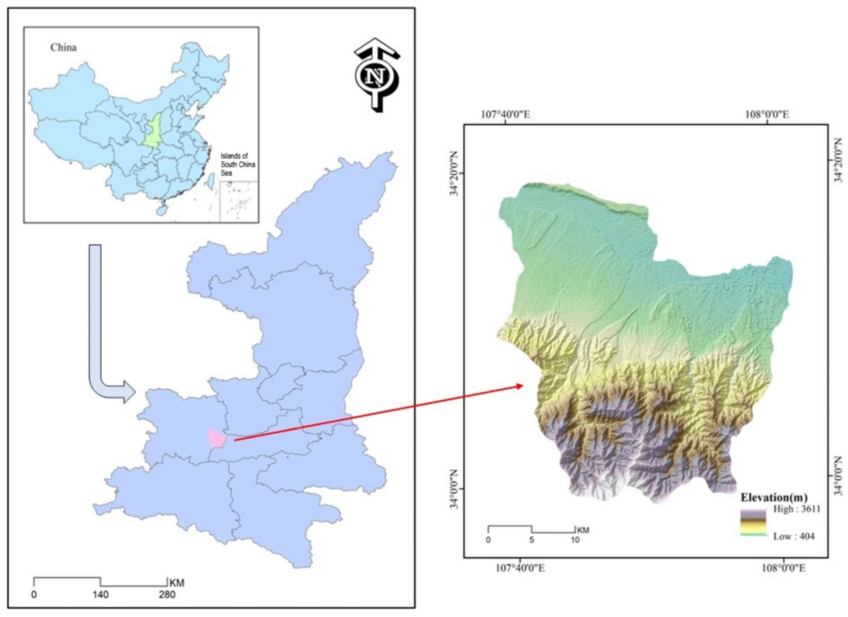
2. Study Area
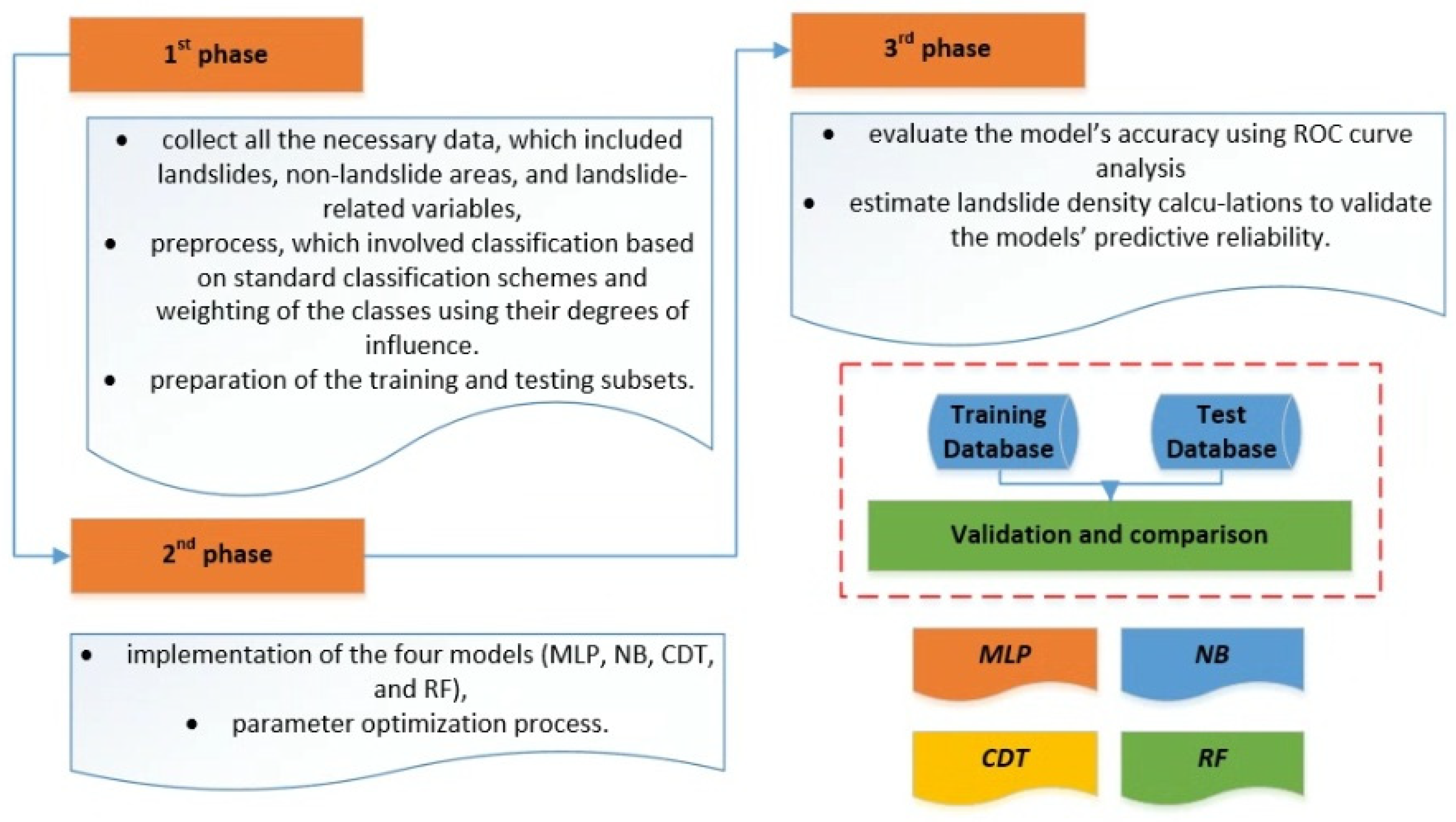
3. Methodology
3.1. First Phase: Data Collection and Preprocessing
3.2. Certainty Factor Method
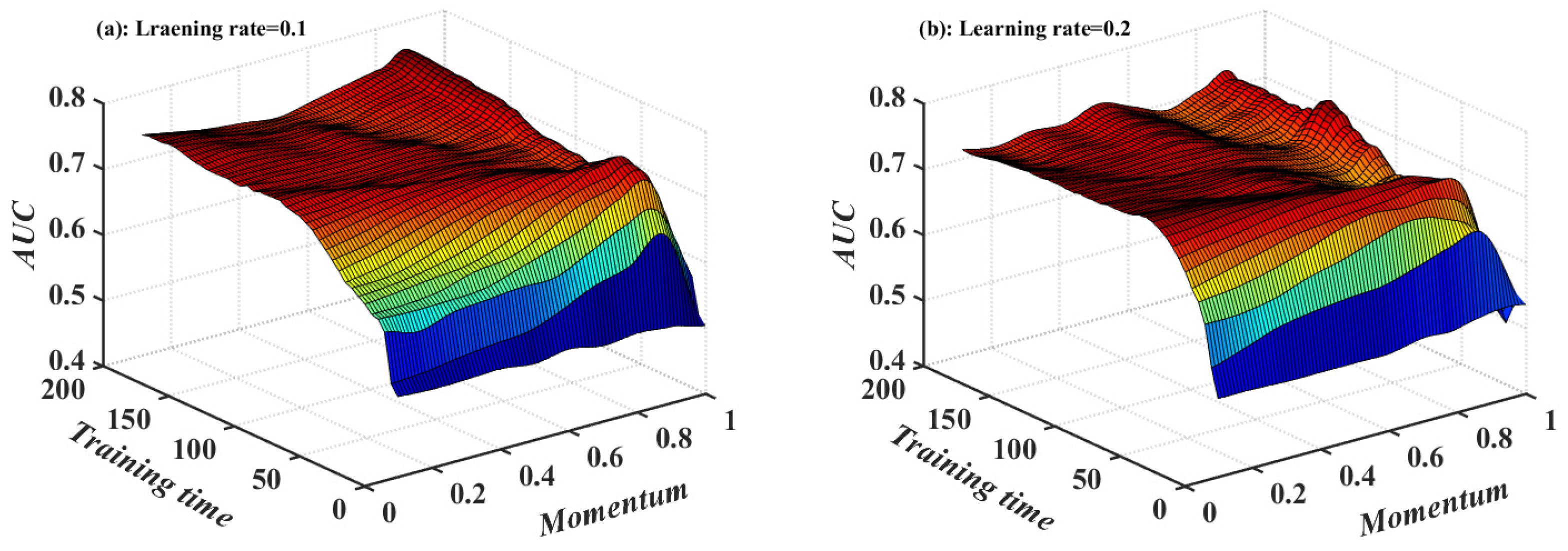
3.3. Multilayer Perceptron
3.4. Naive Bayes
3.5. Credal Decision Trees
3.6. Random Forest
4. Results
4.1. Landslide Conditioning Factor Analysis
4.2. Model Application
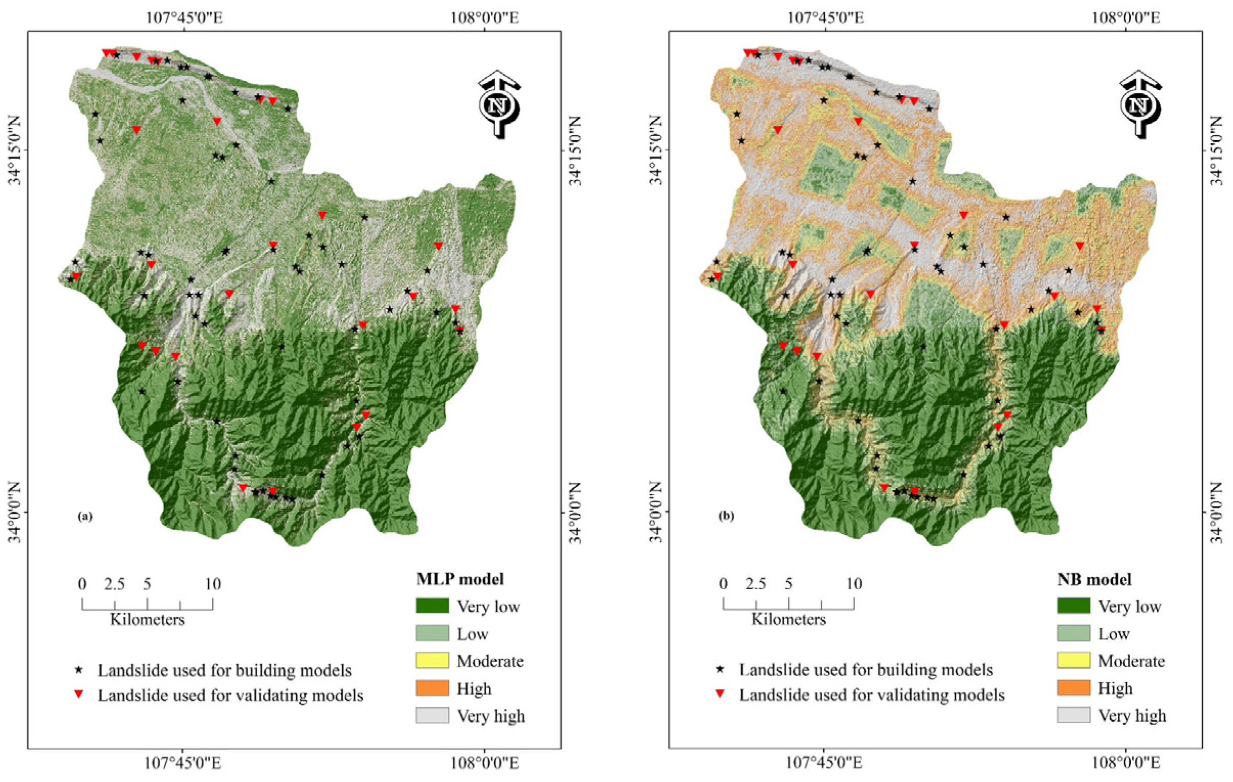
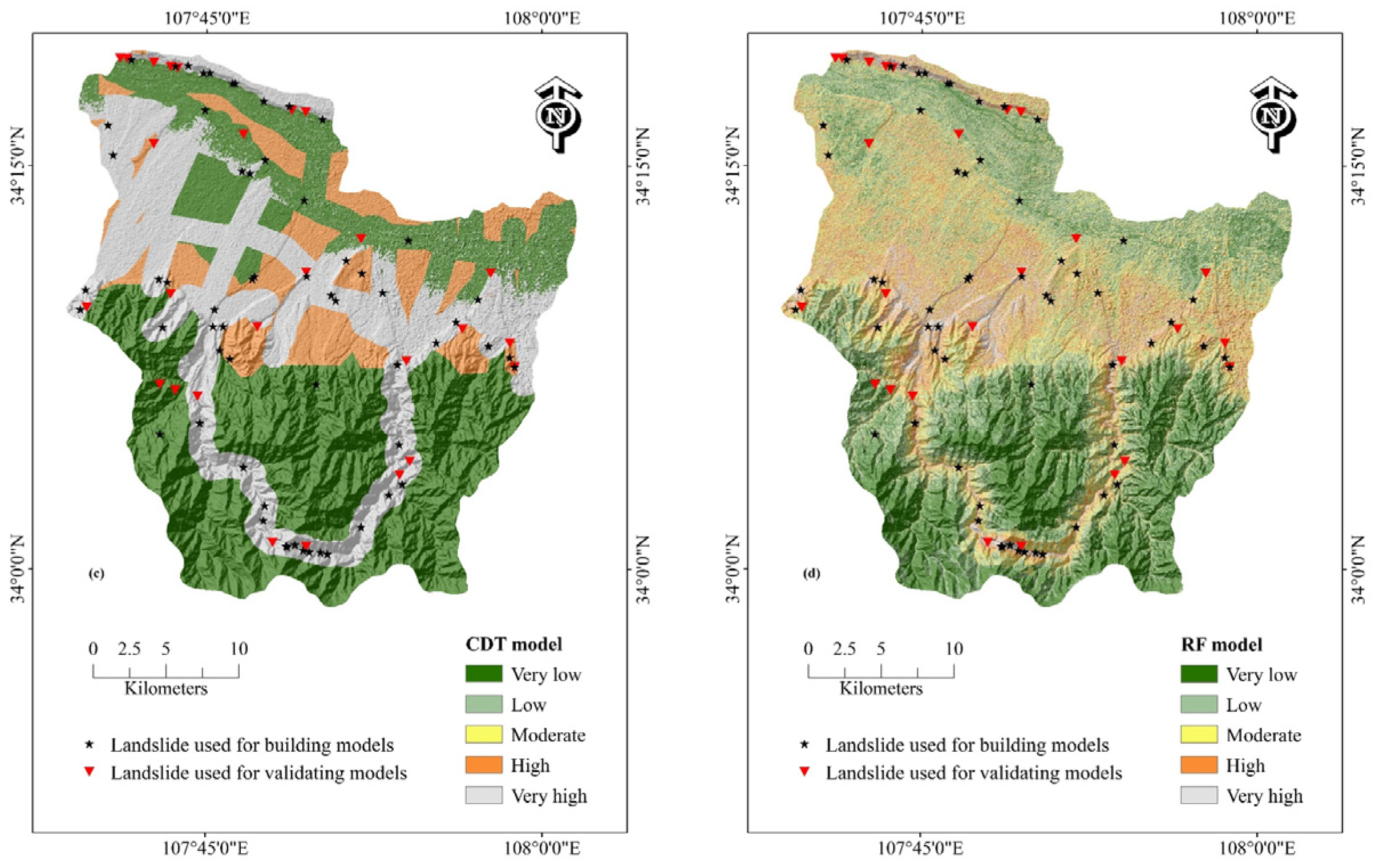
4.3. Generating Landslide Susceptibility Maps
4.4. Validation and Comparison of Models
5. Discussion
6. Conclusions
- Among the many influencing factors, the slope orientation, distance from roads, and land use type are strongly associated with the occurrence of landslides in the study area. This is likely due to geomorphological controls on slope stability and the impact of human activities near road networks. In contrast, the STI, SPI, TWI, and NDVI showed weaker correlations, possibly due to low variability or indirect influence on slope failure mechanisms.
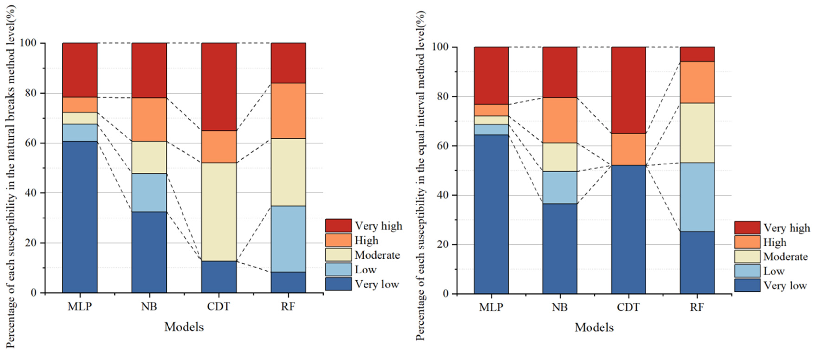
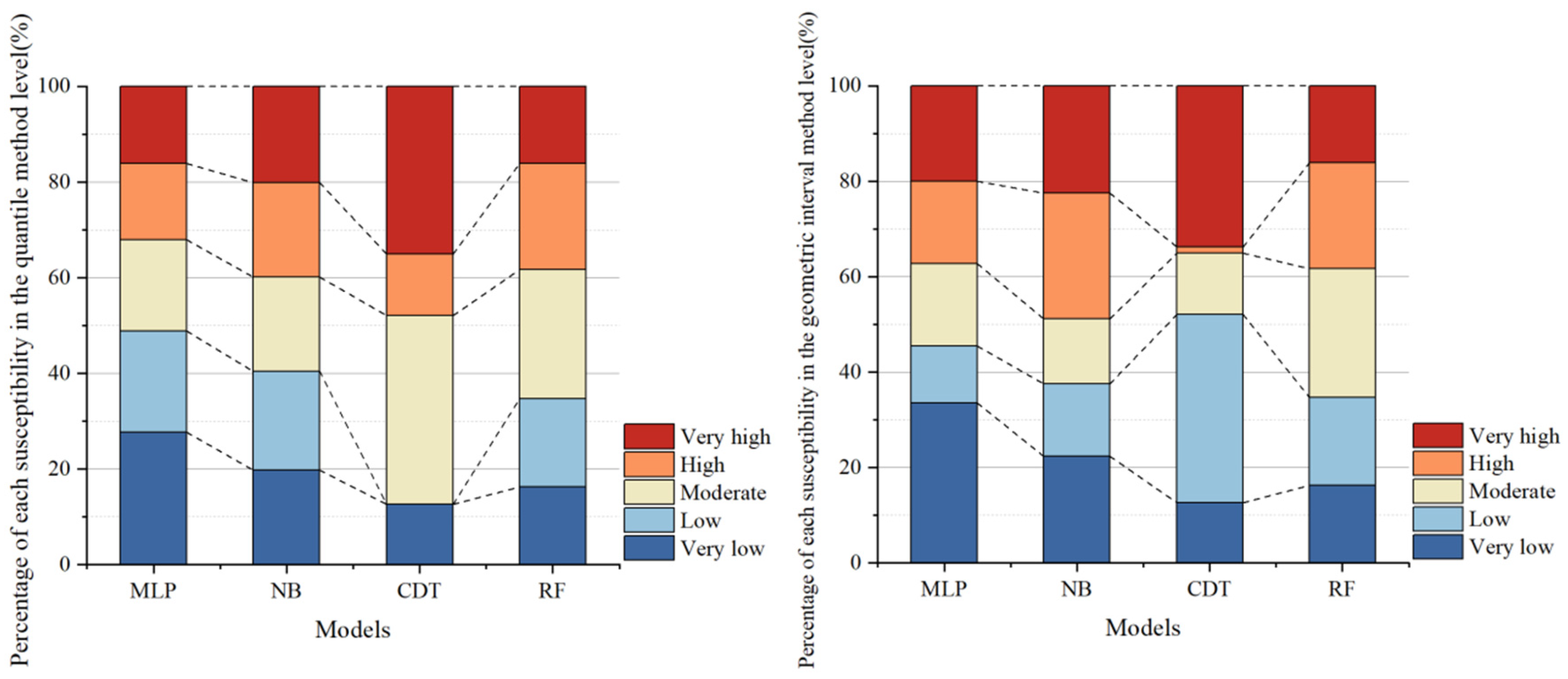
- Four partitioning methods were used to partition the results for each of the four model calculations, and the best results were obtained by using the geometric interval model. This method outperformed others because it effectively handled skewed distributions and enhanced the spatial contrast between susceptibility levels, aligning well with actual landslide occurrences.
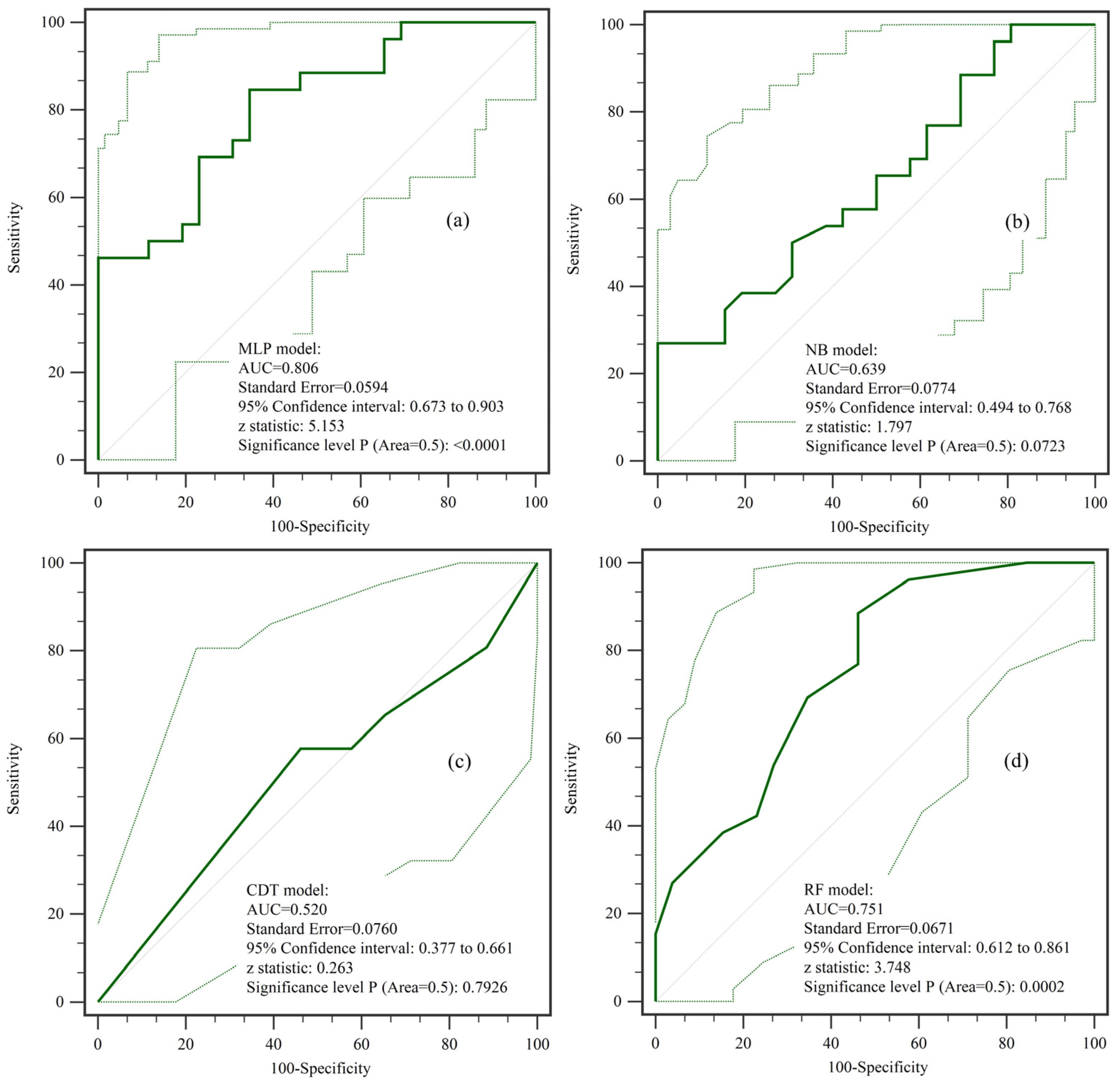
- The CDT model displayed significant segmentation issues in its landslide susceptibility analysis, leading to overly generalized classification results and lower accuracy. This probably stems from its conservative splitting mechanism, which underrepresents spatial heterogeneity. The NB model also showed limitations in its predictive performance, possibly due to its strong independence assumptions among features which rarely hold true in complex terrain. In contrast, the MLP and RF models demonstrated higher reliability and accuracy, making them better suited for landslide susceptibility assessments.
- Based on the LSI distribution, the RF model exhibited the best overall performance, providing well-defined susceptibility zones, due to its ensemble learning structure and robustness to noise. The MLP model effectively highlighted areas of very low and very high landslide susceptibility, offering a more detailed delineation of landslide-prone regions, benefiting from its flexible architecture. The models, ranked from best to worst in terms of performance, are as follows: RF, MLP, NB, and CDT.
Supplementary Materials
Author Contributions
Funding
Institutional Review Board Statement
Informed Consent Statement
Data Availability Statement
Conflicts of Interest
References
- Nguyen, V.V.; Pham, B.T.; Vu, B.T.; Prakash, I.; Jha, S.; Shahabi, H.; Shirzadi, A.; Ba, D.N.; Kumar, R.; Chatterjee, J.M. Hybrid machine learning approaches for landslide susceptibility modeling. Forests 2019, 10, 157. [Google Scholar] [CrossRef]
- Cruden, D.; Novograd, S.; Pilot, G.; Krauter, E.; Bhandari, R.; Cotecchia, V.; Nakamura, H.; Okagbue, C.; Zhuoyuan, Z.; Hutchinson, J. Suggested nomenclature for landslides. Bull. Int. Assoc. Eng. Geol. 1990, 41, 13–16. [Google Scholar]
- Bui, D.T.; Tuan, T.A.; Klempe, H.; Pradhan, B.; Revhaug, I. Spatial prediction models for shallow landslide hazards: A comparative assessment of the efficacy of support vector machines, artificial neural networks, kernel logistic regression, and logistic model tree. Landslides 2016, 13, 361–378. [Google Scholar]
- Chung, C.-J.F.; Fabbri, A.G.; Van Westen, C.J. Multivariate regression analysis for landslide hazard zonation. In Geographical Information Systems in Assessing Natural Hazards; Springer: Berlin/Heidelberg, Germany, 1995; pp. 107–133. [Google Scholar]
- Pourghasemi, H.R.; Pradhan, B.; Gokceoglu, C. Remote Sensing Data Derived Parameters and its Use in Landslide Susceptibility Assessment Using Shannon’s Entropy and GIS. Appl. Mech. Mater. 2012, 225, 486–491. [Google Scholar] [CrossRef]
- Sunil, L.S.; Abraham, M.T.; Satyam, N. Mapping built-up area expansion in landslide susceptible zones using automatic land use/land cover classification. J. Earth Syst. Sci. 2024, 133, 132. [Google Scholar] [CrossRef]
- Kim, J.-C.; Lee, S.; Jung, H.-S.; Lee, S. Landslide susceptibility mapping using random forest and boosted tree models in Pyeong-chang, Korea. Geocarto Int. 2018, 33, 1000–1015. [Google Scholar] [CrossRef]
- Ghorbanzadeh, O.; Rostamzadeh, H.; Blaschke, T.; Gholaminia, K.; Aryal, J. A new gis-based data mining technique using an adaptive neuro-fuzzy inference system (anfis) and k-fold cross-validation approach for land subsidence susceptibility mapping. Nat. Hazards 2018, 94, 497–517. [Google Scholar] [CrossRef]
- Zhang, T.-Y.; Han, L.; Zhang, H.; Zhao, Y.-H.; Li, X.-A.; Zhao, L. Gis-based landslide susceptibility mapping using hybrid integration approaches of fractal dimension with index of entropy and support vector machine. J. Mt. Sci. 2019, 16, 1275–1288. [Google Scholar] [CrossRef]
- Raja, H.; Omar, W.; Mounsif, I. An ensemble modeling of frequency ratio (fr) with evidence belief function (ebf) for gis-based landslide susceptibility mapping: A case study of the coastal cliff of Safi, Morocco. J. Indian Soc. Remote Sens. 2023, 51, 2243–2263. [Google Scholar]
- Dong, J.; Niu, R.; Chen, T.; Dong, L.Y. Assessing landslide susceptibility using improved machine learning methods and considering spatial heterogeneity for the three gorges reservoir area, China. Nat. Hazards 2024, 120, 1113–1140. [Google Scholar] [CrossRef]
- Dipika, K.; Kripamoy, S.; Lal, C.S. Landslide susceptibility mapping in parts of aglar watershed, lesser Himalaya based on frequency ratio method in gis environment. J. Earth Syst. Sci. 2024, 133, 1. [Google Scholar]
- Zhao, X.; Chen, W.; Tsangaratos, P.; Ilia, I. Evaluating landslide susceptibility: The impact of resolution and hybrid integration approaches. Geomat. Nat. Hazards Risk 2024, 15, 2409198. [Google Scholar] [CrossRef]
- Shen, Y.; El Naggar, M.H.; Zhang, D.; Huang, Z.; Du, X. Optimal Intensity Measure for Seismic Performance Assessment of Shield Tunnels in Liquefiable and Non-Liquefiable Soils. Undergr. Space 2025, 21, 149–163. [Google Scholar] [CrossRef]
- Zhao, Z.; Xu, Z.; Hu, C.; Wang, K.; Ding, X. Geographically weighted neural network considering spatial heterogeneity for landslide susceptibility mapping: A case study of Yichang city, China. Catena 2024, 234, 107590. [Google Scholar] [CrossRef]
- Vanani, A.A.G.; Eslami, M.; Ghiasi, Y.; Keyvani, F. Statistical analysis of the landslides triggered by the 2021 sw chelgard earthquake (m l = 6) using an automatic linear regression (linear) and artificial neural network (ann) model based on controlling parameters. Nat. Hazards 2024, 120, 1041–1069. [Google Scholar] [CrossRef]
- Li, Y.; Lin, F.; Luo, X.; Zhu, S.; Li, J.; Xu, Z.; Liu, X.; Luo, S.; Huo, G.; Peng, L. Application of an ensemble learning model based on random subspace and a j48 decision tree for landslide susceptibility mapping: A case study for Qingchuan, Sichuan, China. Environ. Earth Sci. 2022, 81, 267. [Google Scholar] [CrossRef]
- Aastha, S.; Haroon, S.; Hibjur, R.M.; Kanti, S.T.; Nirsobha, B. Effectiveness of hybrid ensemble machine learning models for landslide susceptibility analysis: Evidence from Shimla district of north-west Indian Himalayan region. J. Mt. Sci. 2024, 21, 2368–2393. [Google Scholar]
- Pham, B.T.; Bui, D.T.; Pourghasemi, H.R.; Indra, P.; Dholakia, M. Landslide susceptibility assesssment in the uttarakhand area (india) using gis: A comparison study of prediction capability of na ve bayes, multilayer perceptron neural networks, and functional trees methods. Theor. Appl. Climatol. 2017, 128, 255–273. [Google Scholar] [CrossRef]
- Wang, G.; Lei, X.; Chen, W.; Shahabi, H.; Shirzadi, A. Hybrid computational intelligence methods for landslide susceptibility mapping. Symmetry 2020, 12, 325. [Google Scholar] [CrossRef]
- Trigila, A.; Iadanza, C.; Esposito, C.; Scarascia-Mugnozza, G. Comparison of logistic regression and random forests techniques for shallow landslide susceptibility assessment in Giampilieri (ne Sicily, Italy). Geomorphology 2015, 249, 119–136. [Google Scholar] [CrossRef]
- Lee, S.; Lee, M.-J.; Jung, H.-S.; Lee, S. Landslide susceptibility mapping using na ve bayes and Bayesian network models in Umyeonsan, Korea. Geocarto Int. 2020, 35, 1665–1679. [Google Scholar] [CrossRef]
- Hong, H.; Liu, J.; Bui, D.T.; Pradhan, B.; Acharya, T.D.; Pham, B.T.; Zhu, A.-X.; Chen, W.; Ahmad, B.B. Landslide susceptibility mapping using j48 decision tree with adaboost, bagging and rotation forest ensembles in the Guangchang area (China). Catena 2018, 163, 399–413. [Google Scholar] [CrossRef]
- Pradhan, B. A comparative study on the predictive ability of the decision tree, support vector machine and neuro-fuzzy models in landslide susceptibility mapping using gis. Comput. Geosci. 2013, 51, 350–365. [Google Scholar] [CrossRef]
- Görüm, T. Landslide Recognition and Mapping in a Mixed Forest Environment from Airborne LiDAR Data. Eng. Geol. 2019, 258, 105155. [Google Scholar] [CrossRef]
- Chen, S.; Wu, L.; Miao, Z. Regional seismic landslide susceptibility assessment considering the rock mass strength heterogeneity. Geomat. Nat. Hazards Risk 2023, 14, 1–27. [Google Scholar] [CrossRef]
- Nocentini, N.; Rosi, A.; Piciullo, L.; Liu, Z.; Segoni, S.; Fanti, R. Regional-scale spatiotemporal landslide probability assessment through machine learning and potential applications for operational warning systems: A case study in Kvam (Norway). Landslides 2024, 21, 2369–2387. [Google Scholar] [CrossRef]
- Gokceoglu, C.; Karakas, G.; Zcan, N.T.; Elibuyuk, A.; Kocaman, S. Analysis of landslide susceptibility and potential impacts on infrastructures and settlement areas (A case from the southeastern region of Türkiye). Environ. Earth Sci. 2024, 83, 317. [Google Scholar] [CrossRef]
- Nwazelibe, V.E.; Egbueri, J.C. Geospatial assessment of landslide-prone areas in the southern part of Anambra state, Nigeria using classical statistical models. Environ. Earth Sci. 2024, 83, 220. [Google Scholar] [CrossRef]
- Zhang, G. Landslide susceptibility assessment based on multisource remote sensing considering inventory quality and modeling. Sustainability 2024, 16, 8466. [Google Scholar] [CrossRef]
- Tzampoglou, P.; Loukidis, D.; Anastasiades, A.; Tsangaratos, P. Advanced machine learning techniques for enhanced landslide susceptibility mapping: Integrating geotechnical parameters in the case of Southwestern Cyprus. Earth Sci. Inform. 2025, 18, 357. [Google Scholar] [CrossRef]
- Assiri, M.E.; Ali, M.A.; Siddiqui, M.H.; AlZahrani, A.; Alamri, L.; Alqahtani, A.M.; Ghulam, A.S. Remote sensing assessment of water resources, vegetation, and land surface temperature in eastern Saudi Arabia: Identification, variability, and trends. Remote Sens. Appl. Soc. Environ. 2024, 36, 101296. [Google Scholar] [CrossRef]
- Zezhong, Z.; Kai, Z.; Na, W.; Mingcang, Z.; Zhanyong, H. Machine learning–based systems for early warning of rainfall-induced landslide. Nat. Hazards Rev. 2024, 25, 04024027. [Google Scholar]
- Dai, F.C.; Lee, C.F.; Li, J.; Xu, Z.W. Assessment of landslide susceptibility on the natural terrain of Lantau island, Hong Kong. Environ. Geol. 2001, 40, 381–391. [Google Scholar]
- Sujatha, E.R.; Rajamanickam, G.V.; Kumaravel, P. Landslide susceptibility analysis using probabilistic certainty factor approach: A case study on tevankarai stream watershed, India. J. Earth Syst. Sci. 2012, 121, 1337–1350. [Google Scholar] [CrossRef]
- Ma, W.; Dong, J.; Wei, Z.; Peng, L.; Wu, Q.; Wang, X.; Dong, Y.; Wu, Y. Landslide susceptibility assessment using the certainty factor and deep neural network. Front. Earth Sci. 2023, 10, 1091560. [Google Scholar] [CrossRef]
- Zhang, L.; Pu, H.; Yan, H.; He, Y.; Yao, S.; Zhang, Y.; Ran, L.; Chen, Y. A landslide susceptibility assessment method based on auto-encoder improved deep belief network. Open Geosci. 2023, 15, 20220516. [Google Scholar] [CrossRef]
- Huang, F.; Cao, Z.; Guo, J.; Jiang, S.-H.; Li, S.; Guo, Z. Comparisons of heuristic, general statistical and machine learning models for landslide susceptibility prediction and mapping. Catena 2020, 191, 104580. [Google Scholar] [CrossRef]
- Liu, X.; Shao, S.; Shao, S. Landslide susceptibility prediction and mapping in loess plateau based on different machine learning algorithms by hybrid factors screening: Case study of Xunyi county, Shaanxi province, China. Adv. Space Res. 2024, 74, 192–210. [Google Scholar] [CrossRef]
- Abu Doush, I.; Awadallah, M.A.; Al-Betar, M.A.; Alomari, O.A.; Makhadmeh, S.N.; Abasi, A.K.; Alyasseri, Z.A.A. Archive-based coronavirus herd immunity algorithm for optimizing weights in neural networks. Neural Comput. Appl. 2023, 35, 15923–15941. [Google Scholar] [CrossRef]
- Kaur, R.; Gupta, V.; Chaudhary, B.S. Landslide susceptibility mapping and sensitivity analysis using various machine learning models: A case study of Beas valley, Indian Himalaya. Bull. Eng. Geol. Environ. 2024, 83, 228. [Google Scholar] [CrossRef]
- Melati, D.N.; Umbara, R.P.; Astisiasari, A.; Wisyanto, W. A comparative evaluation of landslide susceptibility mapping using machine learning-based methods in Bogor area of Indonesia. Environ. Earth Sci. 2024, 83, 86. [Google Scholar] [CrossRef]
- Nirbhav; Malik, A.; Maheshwar; Prasad, M.; Saini, A.; Long, N.T. A comparative study of different machine learning models for landslide susceptibility prediction: A case study of Kullu-to-Rohtang pass transport corridor, India. Environ. Earth Sci. 2023, 82, 167. [Google Scholar] [CrossRef]
- Nirbhav; Anand, M.; Maheshwar; Tony, J.; Mukesh, P. Landslide susceptibility prediction based on decision tree and feature selection methods. J. Indian Soc. Remote Sens. 2023, 51, 771–786. [Google Scholar] [CrossRef]
- Dyer, A.S.; Markmoser, M.K.; Duran, R.; Bauer, J.R.; Glade, T.; Murty, T.S. Offshore application of landslide susceptibility mapping using gradient-boosted decision trees: A gulf of Mexico case study. Nat. Hazards 2024, 120, 6223–6244. [Google Scholar] [CrossRef]
- Li, J.; Cao, Z.; Borthwick, A.G.L. Quantifying multiple uncertainties in modelling shallow water-sediment flows: A stochastic galerkin framework with haar wavelet expansion and an operator-splitting approach. Appl. Math. Model. 2022, 106, 259–275. [Google Scholar] [CrossRef]
- Xie, S.; Lin, H.; Duan, H. A novel criterion for yield shear displacement of rock discontinuities based on renormalization group theory. Eng. Geol. 2023, 314, 107008. [Google Scholar] [CrossRef]
- Tracy, F.T.; Vahedifard, F. Analytical solution for coupled hydro-mechanical modeling of infiltration in unsaturated soils. J. Hydrol. 2022, 612, 128198. [Google Scholar] [CrossRef]
- Xia, L.I.; Jiu-Long, C.; De-Hao, Y.U. A methodological framework of landslide quantitative risk assessment in areas with incomplete historical landslide information. J. Mt. Sci. 2023, 20, 2665–2679. [Google Scholar]
- Xia, D.; Tang, H.; Glade, T.; Tang, C.; Wang, Q. Knn-gcn: A deep learning approach for slope-unit-based landslide susceptibility mapping incorporating spatial correlations. Math. Geosci. 2024, 56, 1011–1039. [Google Scholar] [CrossRef]
- Han, M. Spam Filter Based on Naive Bayes Algorithm. In Proceedings of the 5th International Conference on Computing and Data Science (CONF-CDS 2023), Macao, China, 14–15 July 2023; p. 6. [Google Scholar]
- Geng, S.; Li, N.; Zhao, L.; Tian, Y. The method to determine bibliographic types based on decision tree. In Proceedings of the 2016 4th International Conference on Electrical & Electronics Engineering and Computer Science (ICEEECS 2016), Jinan, China, 15–16 October 2016; p. 7. [Google Scholar]
- Wu, S.; Xiong, W. Comparison of different machine learning models in breast cancer. In Proceedings of the 2nd International Conference on Biomedical Engineering, Healthcare and Disease Prevention (BEHDP 2022), Xiamen, China, 28–29 May 2023; p. 6. [Google Scholar]
- Tang, T. Comparison of machine learning methods for estimating customer churn in the telecommunication industry. In Proceedings of the 5th International Conference on Computing and Data Science (CONF-CDS 2023), Macao, China, 14–15 July 2023; p. 6. [Google Scholar]
- Pham, B.T.; Phong, T.V.; Nguyen-Thoi, T.; Trinh, P.T.; Prakash, I. Gis-based ensemble soft computing models for landslide susceptibility mapping. Adv. Space Res. 2020, 66, 1303–1320. [Google Scholar] [CrossRef]
- Arabameri, A.; Pal, S.C.; Rezaie, F.; Chakrabortty, R.; Ngo, P.T.T. Decision tree based ensemble machine learning approaches for landslide susceptibility mapping. Geocarto Int. 2021, 37, 4594–4627. [Google Scholar] [CrossRef]
- Arabameri, A.; Karimi-Sangchini, E.; Pal, S.C.; Saha, A.; Chowdhuri, I.; Lee, S.; Tien Bui, D. Novel credal decision tree-based ensemble approaches for predicting the landslide susceptibility. Remote Sens. 2020, 12, 3389. [Google Scholar] [CrossRef]
- Jingyun, G.; Ignacio, P.; Miao, Y.; Fasuo, Z.; Wei, C. Credal-decision-tree-based ensembles for spatial prediction of landslides. Water 2023, 15, 605. [Google Scholar]
- He, Q.; Xu, Z.; Li, S.; Li, R.; Zhang, S.; Wang, N.; Pham, B.T.; Chen, W. Novel entropy and rotation forest-based credal decision tree classifier for landslide susceptibility modeling. Entropy 2019, 21, 106. [Google Scholar] [CrossRef]
- Nguyen, P.T.; Ha, D.H.; Nguyen, H.D.; Phong, T.V.; Trinh, P.T.; Al-Ansari, N.; Le, H.V.; Pham, B.T.; Ho, L.S.; Prakash, I. Improvement of credal decision trees using ensemble frameworks for groundwater potential modeling. Sustainability 2020, 12, 2622. [Google Scholar] [CrossRef]
- Peter, W. Inferences from multinomial data: Learning about a bag of marbles. J. R. Stat. Soc. Ser. B Methodol. 2018, 58, 3–34. [Google Scholar]
- Breiman, L. Random forests. Mach. Learn. 2001, 45, 5–32. [Google Scholar] [CrossRef]
- Abu El-Magd, S.A.; Ali, S.A.; Pham, Q.B. Spatial modeling and susceptibility zonation of landslides using random forest, naive bayes and k-nearest neighbor in a complicated terrain. Earth Sci. Inform. 2021, 14, 1227–1243. [Google Scholar] [CrossRef]
- Devi, M.; Gupta, V.; Sarkar, K. Landslide susceptibility zonation using integrated supervised and unsupervised machine learning techniques in the Bhagirathi eco-sensitive zone (besz), Uttarakhand, Himalaya, India. J. Earth Syst. Sci. 2024, 133, 131. [Google Scholar] [CrossRef]
- Tanyu, B.F.; Aiyoub, A.; Yashar, A.; Gheorghe, T. Landslide susceptibility analyses using random forest, c4.5, and c5.0 with balanced and unbalanced datasets. Catena 2021, 203, 105355. [Google Scholar] [CrossRef]
- Wang, R. Predicting pulse wave age from cardiovascular characteristics using machine learning algorithms. In Proceedings of the 5th International Conference on Computing and Data Science (CONF-CDS 2023), Macao, China, 14–15 July 2023; p. 8. [Google Scholar]
- Bikesh, M.; Canh, H.T.; Kumar, B.P.; Suchita, S.; Singh, P.A.M. Soft computing machine learning applications for assessing regional-scale landslide susceptibility in the Nepal Himalaya. Eng. Comput. 2024, 41, 655–681. [Google Scholar]
- Qiqing, W.; Yinghai, G.; Wenping, L.; Jianghui, H.; Zhiyong, W. Predictive modeling of landslide hazards in wen county, northwestern China based on information value, weights-of-evidence, and certainty factor. Geomat. Nat. Hazards Risk 2019, 10, 820–835. [Google Scholar]
- Dingying, Y.; Ting, Z.; Alireza, A.; Santosh, M.; Deep, S.U.; Aznarul, I. Flash-flood susceptibility mapping: A novel credal decision tree-based ensemble approaches. Earth Sci. Inform. 2023, 16, 3143–3161. [Google Scholar]
- Barman, J.; Das, J. Assessing classification system for landslide susceptibility using frequency ratio, analytical hierarchical process and geospatial technology mapping in Aizawl district, ne India. Adv. Space Res. 2024, 74, 1197–1224. [Google Scholar] [CrossRef]
- Saito, H.; Nakayama, D.; Matsuyama, H. Relationship between the initiation of a shallow landslide and rainfall intensity—Duration thresholds in Japan—Sciencedirect. Geomorphology 2010, 118, 167–175. [Google Scholar] [CrossRef]
- Ozturk, D.; Uzel-Gunini, N. Investigation of the effects of hybrid modeling approaches, factor standardization, and categorical mapping on the performance of landslide susceptibility mapping in van, turkey. Nat. Hazards 2022, 114, 2571–2604. [Google Scholar] [CrossRef]
- Adugna, M.A.; Kumar, R.T.; Venkata, S.K.; Tibebu, K. Gis-based landslide susceptibility zonation and risk assessment in complex landscape: A case of Beshilo watershed, northern Ethiopia. Environ. Chall. 2022, 8, 100586. [Google Scholar]
- Xinzhi, Z.; Haijia, W.; Yalan, Z.; Jiahui, X.; Wengang, Z. Landslide susceptibility mapping using hybrid random forest with geodetector and rfe for factor optimization. Geosci. Front. 2021, 12, 101211. [Google Scholar]
- Capitani, M.; Ribolini, A.; Bini, M. The slope aspect: A predisposing factor for landsliding? Comptes Rendus Géosci. 2013, 345, 427–438. [Google Scholar] [CrossRef]
- Reichenbach, P.; Rossi, M.; Malamud, B.D.; Mihir, M.; Guzzetti, F. A review of statistically-based landslide susceptibility models. Earth Sci. Rev. 2018, 180, 60–91. [Google Scholar] [CrossRef]
- Ghosh, S.; Carranza, E.J.M.; van Westen, C.J.; Jetten, V.G.; Bhattacharya, D.N. Selecting and weighting spatial predictors for empirical modeling of landslide susceptibility in the Darjeeling Himalayas (India). Geomorphology 2011, 131, 35–56. [Google Scholar] [CrossRef]
- Yi, Y.; Zhang, Z.; Zhang, W.; Jia, H.; Zhang, J. Landslide susceptibility mapping using multiscale sampling strategy and convolutional neural network: A case study in Jiuzhaigou region. Catena 2020, 195, 104851. [Google Scholar] [CrossRef]
- Goetz, J.; Brenning, A.; Petschko, H.; Leopold, P. Evaluating machine learning and statistical prediction techniques for landslide susceptibility modelling. Comput. Geosci. 2015, 81, 1–11. [Google Scholar] [CrossRef]
- Chen, Y. Spatial prediction and mapping of landslide susceptibility using machine learning models. Nat. Hazards 2025, 121, 8367–8385. [Google Scholar] [CrossRef]
- Tsangaratos, P.; Ilia, I. Comparison of a logistic regression and naive Bayes classifier in landslide susceptibility assessments: The influence of models complexity and training dataset size. Catena 2016, 145, 164–179. [Google Scholar] [CrossRef]
- Kakavas, M.P.; Nikolakopoulos, K.G. Digital Elevation Models of Rockfalls and Landslides: A Review and Meta-Analysis. Geosciences 2021, 11, 256. [Google Scholar] [CrossRef]
- Kakavas, M.P.; Frattini, P.; Previati, A.; Nikolakopoulos, K.G. Evaluating the Impact of DEM Spatial Resolution on 3D Rockfall Simulation in GIS Environment. Geosciences 2024, 14, 200. [Google Scholar] [CrossRef]
- Mahalingam, R.; Olsen, M.J.; O’Banion, M.S. Evaluation of Landslide Susceptibility Mapping Techniques Using LiDAR-Derived Conditioning Factors (Oregon Case Study). Geomat. Nat. Hazards Risk 2016, 7, 1884–1907. [Google Scholar] [CrossRef]
- Corominas, J.; van Westen, C.; Frattini, P.; Cascini, L.; Malet, J.P.; Fotopoulou, S.; Catani, F.; Van Den Eeckhaut, M.; Mavrouli, O.; Agliardi, F.; et al. Recommendations for the Quantitative Analysis of Landslide Risk. Bull. Eng. Geol. Environ. 2014, 73, 209–263. [Google Scholar] [CrossRef]
- Martha, T.; Kerle, N.; van Westen, C.J.; Kumar, K.V. Characterising Spectral, Spatial and Morphometric Properties of Landslides for Semi-Automatic Detection Using Object-Oriented Methods. Geomorphology 2010, 116, 24–36. [Google Scholar] [CrossRef]
- Kazemi, F.; Asgarkhani, N.; Jankowski, R. Optimization-Based Stacked Machine-Learning Method for Seismic Probability and Risk Assessment of Reinforced Concrete Shear Walls. Expert Syst. Appl. 2024, 255, 124897. [Google Scholar] [CrossRef]


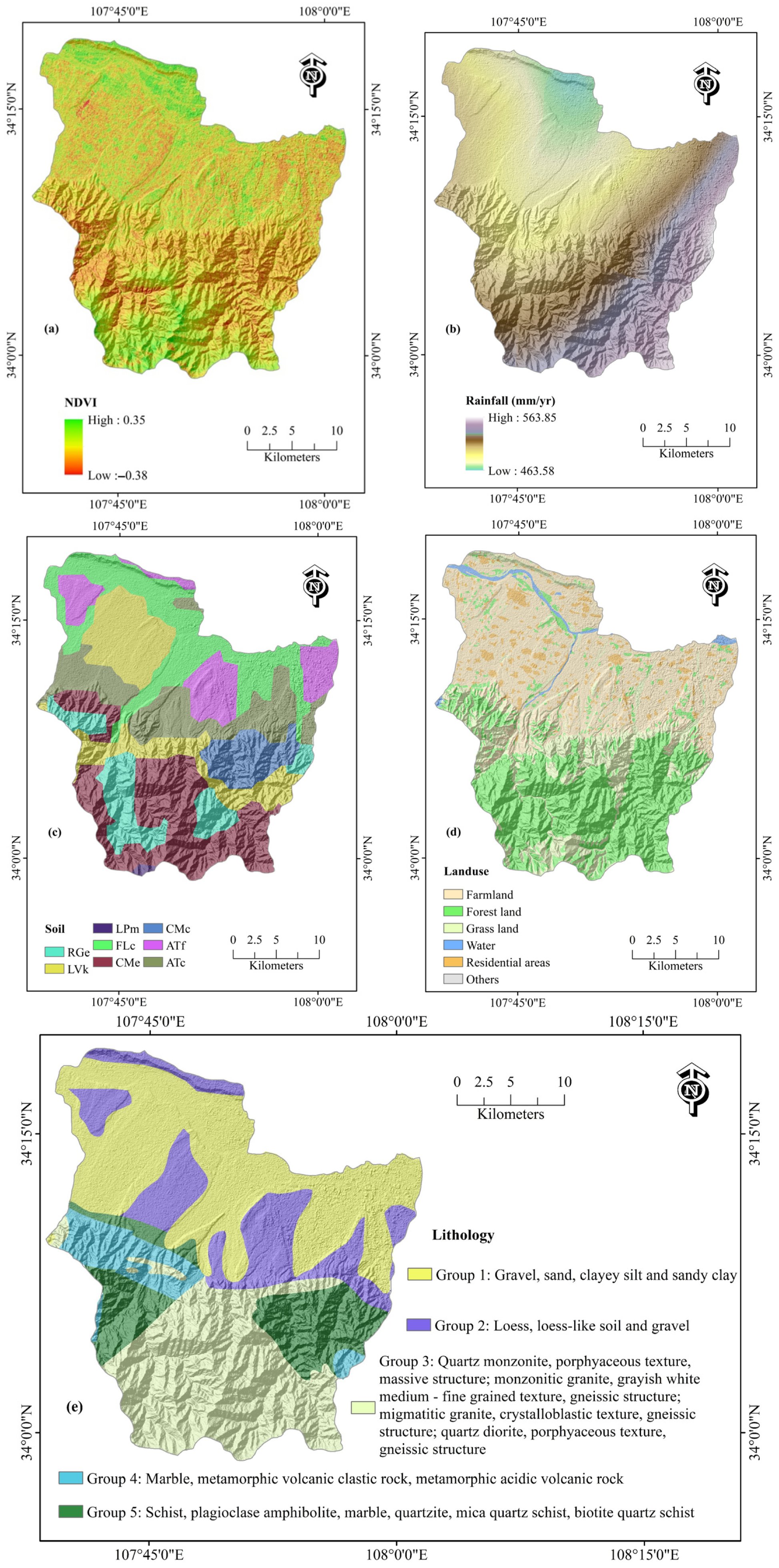
| Factor Category | Factor | Classifications/Ranges |
|---|---|---|
| Topographic | Slope (°) | 0.00–8.72, 8.72–19.19, 19.19–30.82, 30.82–43.32, 43.32–74.13 |
| Aspect | North, Northeast, East, Southeast, South, Southwest, West, Northwest | |
| Elevation (m) | 422–798, 798–1281, 1281–1818, 1818–2399, 2399–3648 | |
| Hydrological/Terrain Indices | STI | <18.25, 18.25–66.91, 66.91–164.22, 164.22–352.78, >352.78 |
| SPI | <20.47, 20.47–88.80, 88.80–232.30, 232.30–573.93, >573.93 | |
| TWI | <1.73, 1.73–2.66, 2.66–6.44, 6.44–10.22, >10.22 | |
| Plan Curvature | −28.23 to −0.05, −0.05 to 0.05, 0.05 to 25.33 | |
| Profile Curvature | −34.05 to −0.05, −0.05 to 0.05, 0.05 to 32.55 | |
| Proximity Factors | Distance to Faults (m) | 0–500, 500–1000, 1000–1500, 1500–2000, >2000 |
| Distance to Roads (m) | 0–300, 300–600, 600–900, 900–1200, >1200 | |
| Climatic | Rainfall (mm/year) | 463.58–484.42, 484.42–500.94, 500.94–518.63, 518.63–537.50, 537.50–563.85 |
| Land Use | Type | Farmland, Forest land, Grassland, Water bodies, Residential areas, Others |
| Soil Type | Soil Class | Eutric Regosol, Calcic Luvisol, Mollic Leptosol, Calcaric Fluvisol, Eutric Cambisol, Calcaric Cambisol, Fimic Anthrosol, Cumulic Anthrosol |
| Geological | Lithology Group | Group 1: Gravel/sand/clayey silt, Group 2: Loess, Group 3: Granite/gneiss, Group 4: Marble/volcanic rocks, Group 5: Schist/quartzite |
Disclaimer/Publisher’s Note: The statements, opinions and data contained in all publications are solely those of the individual author(s) and contributor(s) and not of MDPI and/or the editor(s). MDPI and/or the editor(s) disclaim responsibility for any injury to people or property resulting from any ideas, methods, instructions or products referred to in the content. |
© 2025 by the authors. Licensee MDPI, Basel, Switzerland. This article is an open access article distributed under the terms and conditions of the Creative Commons Attribution (CC BY) license (https://creativecommons.org/licenses/by/4.0/).
Share and Cite
Zhang, C.; Liu, D.; Tsangaratos, P.; Ilia, I.; Ma, S.; Chen, W. Enhancing Predictive Accuracy of Landslide Susceptibility via Machine Learning Optimization. Appl. Sci. 2025, 15, 6325. https://doi.org/10.3390/app15116325
Zhang C, Liu D, Tsangaratos P, Ilia I, Ma S, Chen W. Enhancing Predictive Accuracy of Landslide Susceptibility via Machine Learning Optimization. Applied Sciences. 2025; 15(11):6325. https://doi.org/10.3390/app15116325
Chicago/Turabian StyleZhang, Chuanwei, Dingshuai Liu, Paraskevas Tsangaratos, Ioanna Ilia, Sijin Ma, and Wei Chen. 2025. "Enhancing Predictive Accuracy of Landslide Susceptibility via Machine Learning Optimization" Applied Sciences 15, no. 11: 6325. https://doi.org/10.3390/app15116325
APA StyleZhang, C., Liu, D., Tsangaratos, P., Ilia, I., Ma, S., & Chen, W. (2025). Enhancing Predictive Accuracy of Landslide Susceptibility via Machine Learning Optimization. Applied Sciences, 15(11), 6325. https://doi.org/10.3390/app15116325