Effects of Discrete Thrust Levels on the Trajectory Design of the BIT-3 RF Ion Thruster-Equipped CubeSat

Abstract

The use of continuous-thrust propulsion systems allows spacecraft to cover complex space trajectories and to complete missions that would be difficult using chemical thrusters. Among the continuous-thrust propulsion systems proposed in recent decades, solar electric thrusters occupy an important position thanks to the maturity reached by this technology. Technological advances in the miniaturization of spacecraft components allow an electric thruster to be installed even in a small and standardized vehicle such as a CubeSat. In this context, the BIT-3 RF ion thruster is an interesting option that has been recently employed in some space missions for the study of the lunar surface. In the recent literature, the performance of a CubeSat equipped with a propulsion system based on the BIT-3 has been studied considering a simplified model in which the thrust magnitude has a fixed value or varies continuously within a prescribed range. However, the operating levels of a BIT-3 are finite in number. This paper studies the transfer performance of a BIT-3-propelled CubeSat considering the actual operating levels that can be provided by such a thruster. The work analyzes the optimal transfer towards asteroid 2000 SG344 when the electric power is obtained through solar arrays.

1. Introduction

The use of advanced space propulsion systems, which are able to give a steerable thrust vector, whose magnitude can be selected within a prescribed range during the flight, allows robotic spacecraft to cover complex, non-Keplerian, space trajectories and to complete scientific missions that would be difficult using more common chemical thrusters, both in planetocentric and heliocentric contexts [1,2,3,4,5]. Among the continuous-thrust propulsion systems proposed or actually used in recent decades, such as the well-known photonic solar sails [6,7,8] or the more exotic electric solar wind sails [9,10,11,12], solar electric thrusters actually occupy a prominent position thanks to the maturity reached by this specific important technology [13,14,15]. This maturity has allowed its operational use as a primary propulsion system, even in challenging interplanetary scenarios, since NASA’s mission Deep Space 1 launched almost thirty years ago [16,17,18,19]. In addition, the continuous and throttleable propulsive acceleration vector provided by a solar electric thruster has also been proposed for the de-orbiting of small satellites [20,21], or for achieving an optimal reconfiguration and maintenance of complex spacecraft formation structures [22,23,24].

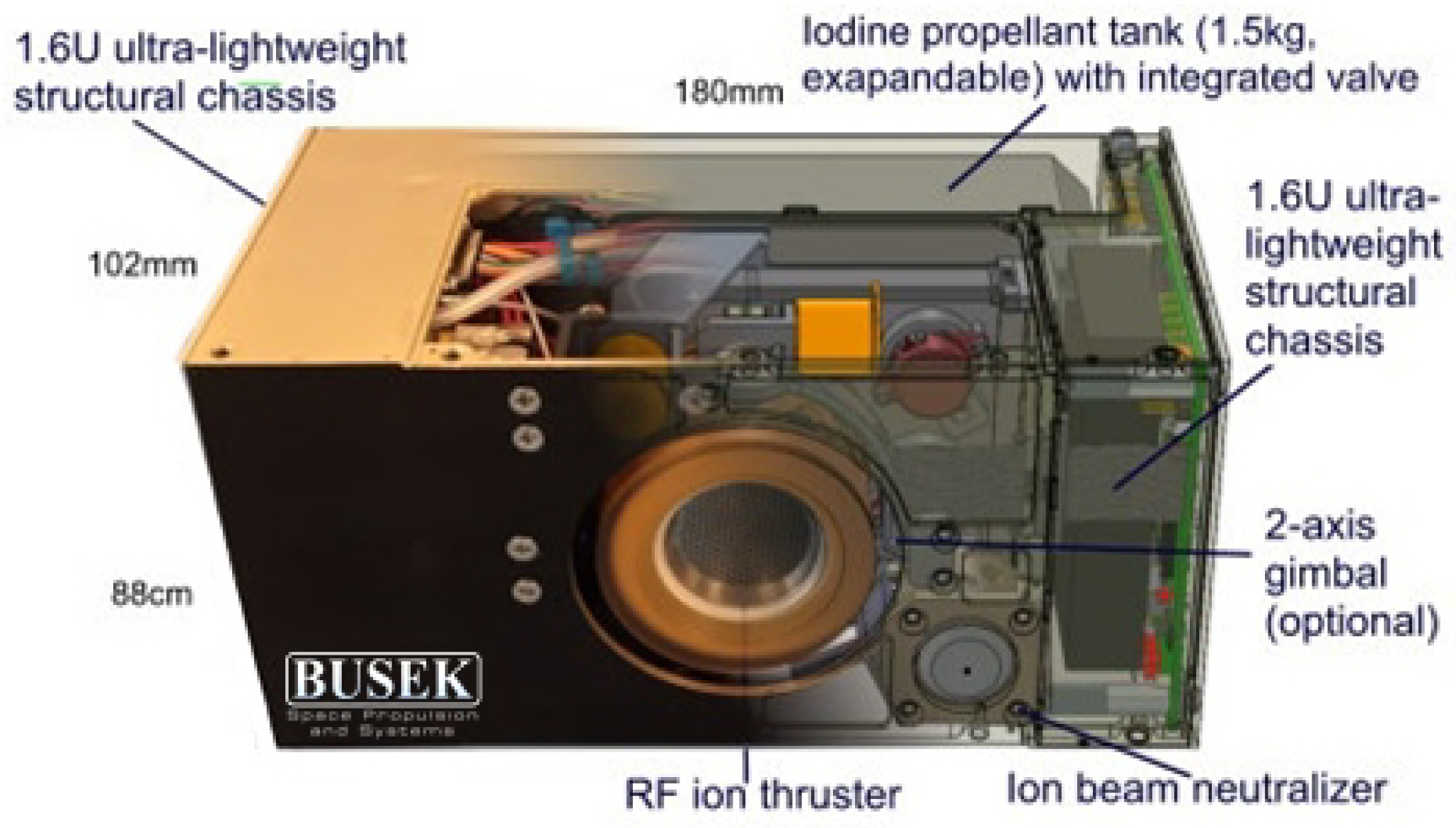
Technological advances in the miniaturization of both spacecraft components [25] and scientific payloads [26,27] have recently enabled the installation of a continuous-thrust propulsion system on board a CubeSat [28], such as a medium-sized photonic solar sail [29,30,31] or a miniaturized solar electric thruster [32]. In this context, the Busek’s BIT-3 RF ion thruster (Busek Co. Inc., Natick, MA, USA) represents an interesting, efficient, and compact iodine gridded engine that allows us to achieve a maximum thrust magnitude of about 1.1 mN, with a specific impulse of 2150 s and a rather small occupied volume of 1.6 U [33]. A cutaway of the BIT-3 engine unit, which also houses a propellant tank with 1.5 kg of solid iodine, is shown in Figure 1. In this figure, one can observe the presence of a two-axis gimbal system that allows the (possibly) small spacecraft’s reaction wheels to be desaturated. The technology readiness level achieved by this type of miniaturized RF ion thruster [34,35,36] allowed its operational use in two scientific space missions launched by NASA a few years ago, that is, the Lunar Polar Hydrogen Mapper (LunaH-Map) [37] and the Lunar IceCube [38,39], which were designed to perform remote sensing of the lunar surface using two (small) 6 U CubeSats whose launch mass was 14 kg.

In the recent literature, the performance of a CubeSat equipped with a propulsion system based on the BIT-3 thruster technology has been studied considering a simplified mathematical model in which the thrust magnitude has a fixed value during the flight [40] or varies continuously within a prescribed range [41] as a function of the available input power given by a solar array-based subsystem [42]. However, the operating levels and the performance characteristics of a BIT-3 engine unit, in terms of specific impulse and the electric power required for the system to function, are finite in number, according to the typical thrust table of the electric thruster which can be retrieved from the recent works of Tsay et al. [43,44]. In particular, as detailed in Section 2, according to Ref. [44], the thrust table of the BIT-3 RF ion engine has five distinct operating levels to which a sixth is added that, although technically a thrust command, can be considered a sort of fictitious thrust level, as it produces almost zero thrust while consuming a small amount of propellant. This additional fictitious operating level is inserted into the actual thrust table to model a BIT-3 operating condition in which the engine unit is essentially in a sort of idle mode that, however, allows it to reach normal thrust conditions without going through the entire ignition sequence [44]. The BIT-3 engine unit also has two other operating modes, in addition to the one called “thrust mode” (TM) [43,44]. In fact, it is possible to insert the engine unit into a so-called “sleep mode” (SM) in which the electric power absorbed is the minimum (a value of about 3.2 W, which is required for communication), while the TM is preceded by a “warm standby mode” (WSM), which absorbs an electric power up to a maximum of 30 W (with a value of about 20 W to maintain the mode), which serves to prepare the propulsion system to provide the required operating level indicated in the actual thrust table.

The aim of this paper is to study the space trajectory and the guidance laws of a classical CubeSat equipped with a BIT-3 RF ion thruster as primary propulsion system, taking into account the actual (few) operating levels that can be provided by such an electric engine according to its thrust table [44]. In this context, as discussed in Section 3, this paper considers a typical heliocentric mission scenario in which a BIT-3-propelled interplanetary CubeSat transfers between two assigned Keplerian orbits [45]. In particular, analyzing the orbital transfer problem in an optimization framework, this paper discusses the optimal guidance laws of the BIT-3-propelled small spacecraft as a function of the available electric power obtained through a high-performance solar panel-based subsystem [42]. In this context, an indirect approach [46,47,48] is used to design the CubeSat’s transfer trajectory towards asteroid 2000 SG344, while the Pontryagin’s Maximum Principle (PMP) [49] is employed to obtain the optimal control law in terms of both the thrust vector direction and the operating level selection. The numerical results of the simulations are illustrated in Section 4, which also contains a parametric study of the optimal transfer performance as a function of the CubeSat’s reference electric power. Finally, Section 5 contains the concluding remarks.

2. BIT-3 Thrust Model for Preliminary Mission Analysis

In this section, the thrust model of a BIT-3 engine unit is analyzed assuming a TM and considering the admissible operating levels given in the engine’s thrust table. To this end, the mathematical model considers the thruster data indicated in Ref. [44], which gives the BIT-3 performances in terms of thrust magnitude T, the Power Processing Unit (PPU) input power P, the specific impulse $I_{\mathrm{sp}}$, and the screen grid current C. In particular, Tsay [44] indicates the value of the set $\{T,P,I_{\mathrm{sp}},C\}$ for six possible operating levels (the generic operating level is indicated by the symbol $\mathrm{Id}\in {\mathbb{N}}_0$), as reported in

Table 1. BIT-3 thrust table as indicated in Ref. [44], when the engine unit is in TM. The operating level $\mathrm{Id}=0$ indicates a condition in which the amount of thrust is substantially zero. Data retrieved from Ref. [44].

$\mathbf{Id}$	T [mN]	P [W]	${\mathit{I}}_{\mathbf{sp}}$ [s]	C [mA]
0	$0.01$	42	20	0
1	$0.66$	55	1290	$9.9$
2	$0.78$	60	1530	$11.4$
3	$0.89$	65	1740	$12.9$
4	$1.00$	70	1960	$14.3$
5	$1.10$	75	2150	$15.6$

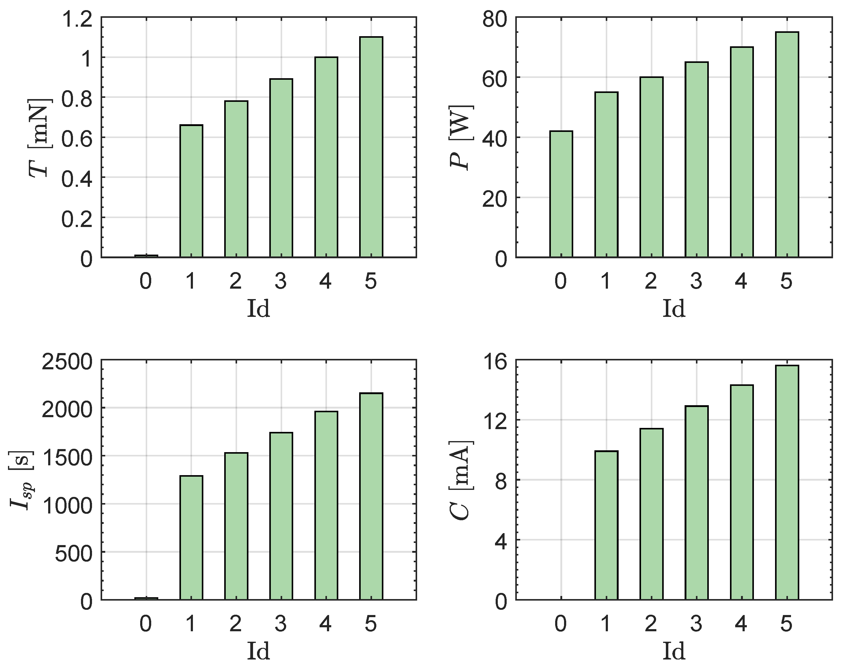
, which coincides with the engine unit’s thrust table in this work. Figure 2 shows the bar plot of the BIT-3 performance characteristics $\{T,P,I_{\mathrm{sp}},C\}$ as a function of the operating level $\mathrm{Id}=[0,1,2,3,4,5]$.

From Table 1 or Figure 1, it can be observed that the operating level $\mathrm{Id}=0$ substantially corresponds to a zero-thrust condition in which the electric power required for the operation of the solar electric thruster is nevertheless non-zero, amounting to 42 W. Furthermore, the value of the specific impulse $I_{\mathrm{sp}}$ relative to the operating level $\mathrm{Id}=0$ is non-zero, even though it is extremely small (the value is in fact just 20 s). This non-zero value of $I_{\mathrm{sp}}$ indicates, as explicitly observed by Tsay [44], that there is propellant consumption and electric power waste even in the condition of $\mathrm{Id}=0$, which gives in fact practically zero thrust. In accordance with what was discussed in the Introduction Section, $\mathrm{Id}=0$ indicates the so-called fictitious level which models the zero-thrust condition, and which is in addition to the five effective operating levels ${\mathrm{Id}}_e\triangleq [1,2,3,4,5]$ which provide an effective condition where the BIT-3 engine unit provides appreciable thrust.

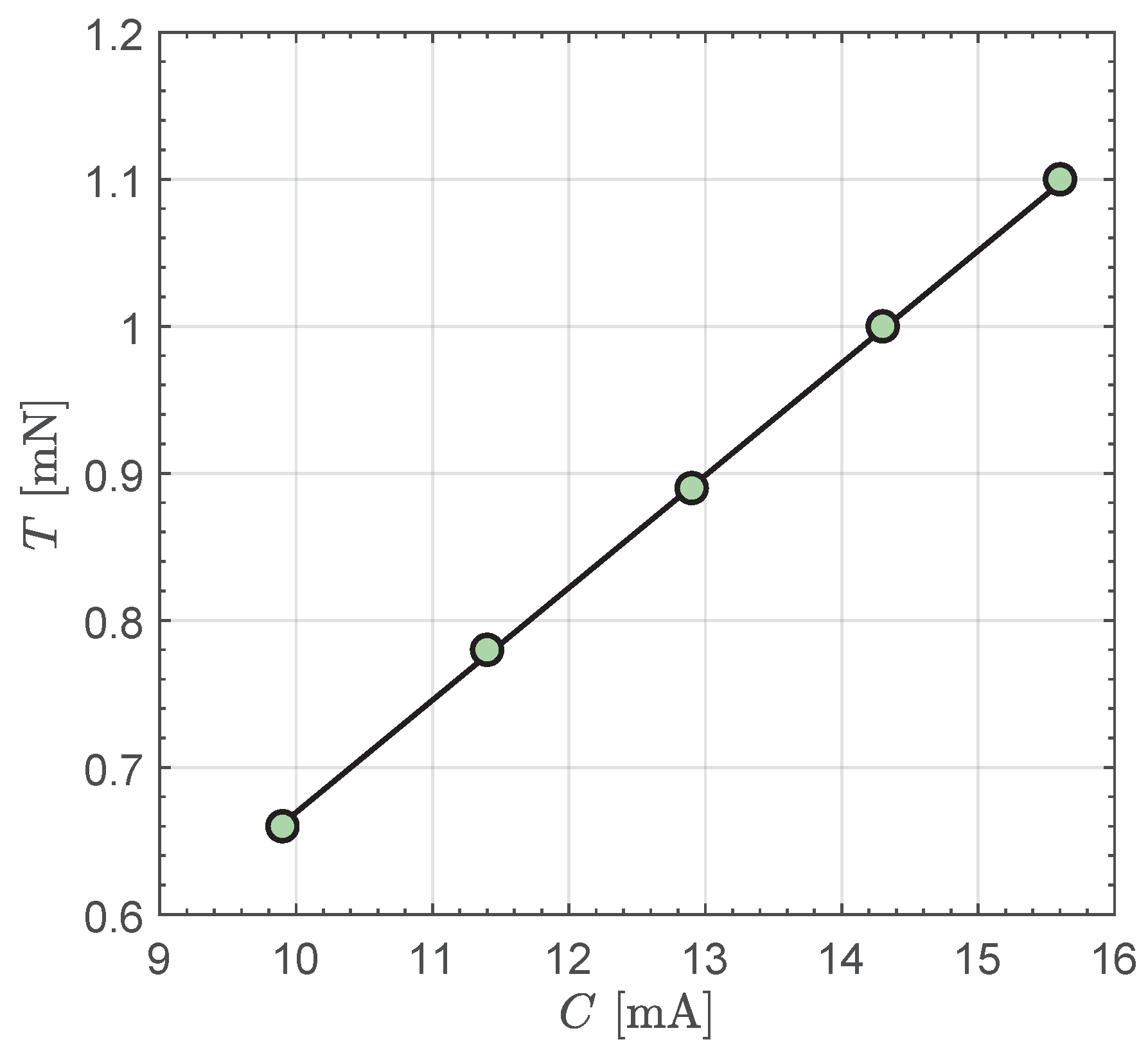
The last column of Table 1 summarizes the screen grid current C required by each operating level. In particular, the thrust magnitude T exhibits a nearly linear variation with the screen grid current. In fact, as suggested in Ref. [44], the function $T=T\left(C\right)$ when $\mathrm{Id}\equiv {\mathrm{Id}}_e$ can be accurately approximated by the following linear equation:

$$T\simeq 0.0764 \left(C-0.1\right)-0.087\mathrm{with}C\in [9.9, 15.6] \mathrm{mA}$$

(1)

where C is milliampere and T is in millinewton.

The linear relation in the preceding equation, which is shown in Figure 3, can be used to express in simple analytical form the amount of thrust as a function of C, so that the screen grid current can be considered as a sort of (continuous) scalar control variable that can be used to select the other performance parameters of the BIT-3 engine unit during the flight. In this work, instead, the chosen control variable corresponds to the operating level $\mathrm{Id}$, which provides through Table 1 the effective values of the performance parameters of the electric propulsion system. It is therefore a discrete dimensionless control variable, which clearly involves a complication in the definition of the control law during a generic orbital transfer, since the thrust magnitude and the mass consumption of the small spacecraft do not have, in general, a continuous variation in time, as will be discussed later in the paper.

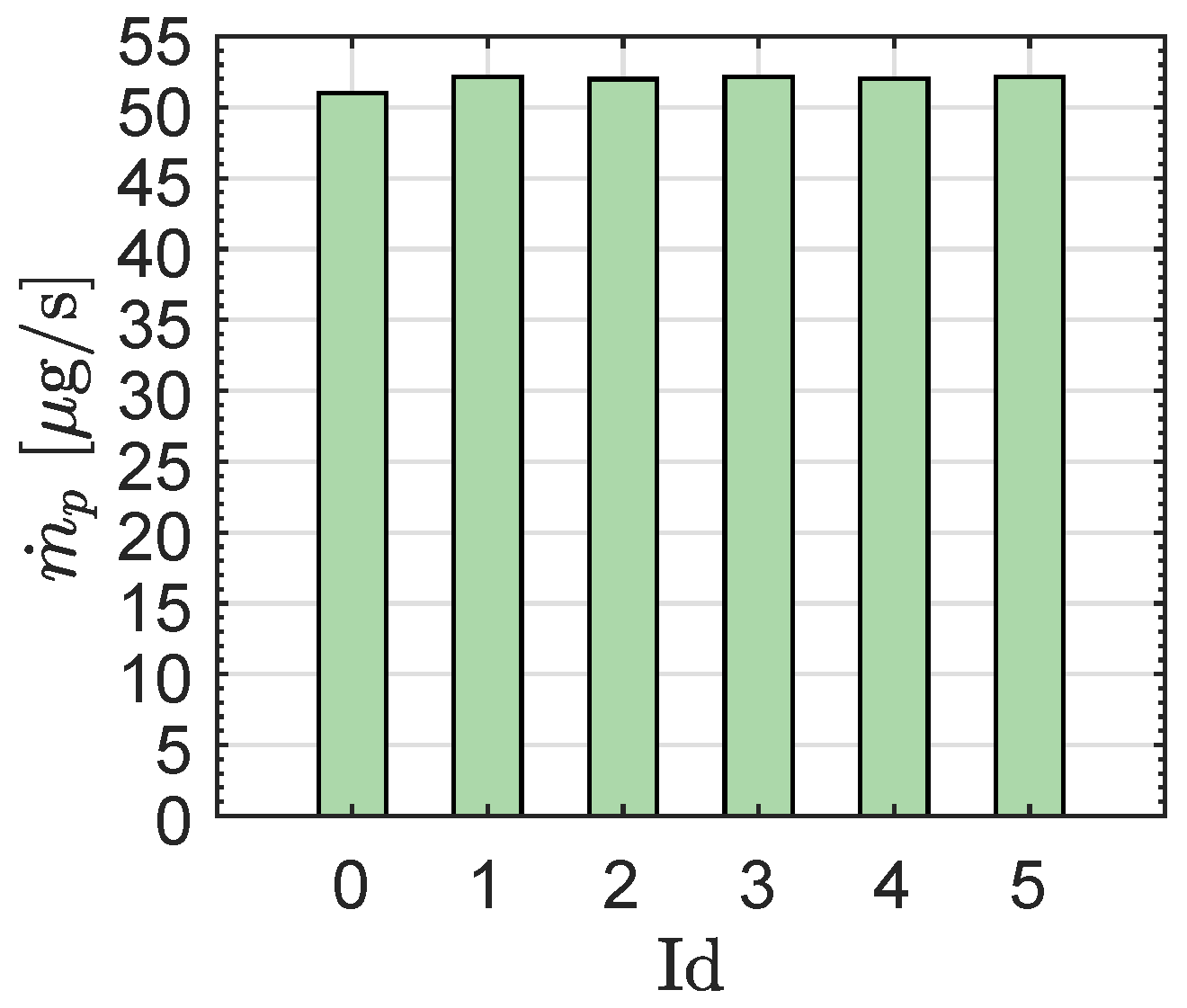
The propellant mass flow rate ${\dot{m}}_p$ which gives, apart from the sign, the temporal variation of the spacecraft total mass m, can be determined as a function of the control variable $\mathrm{Id}$ using the data summarized in Table 1. In this context, indicating with $g_0=9.80665 \mathrm{m}/{\mathrm{s}}^2$ the standard gravity and using the following (well-known) equation

$${\dot{m}}_p={\displaystyle \frac{T}{g_0 I_{\mathrm{sp}}}}$$

(2)

one obtains the results summarized in

Table 2. Propellant mass flow rate ${\dot{m}}_p$ as a function of the engine unit’s operating level $\mathrm{Id}$; see also Equation (2) and Table 1.

$\mathbf{Id}$	${\dot{\mathit{m}}}_{\mathit{p}}$ [μg/s]
0	$50.98$
1	$52.17$
2	$51.98$
3	$52.15$
4	$52.02$
5	$52.17$

and Figure 4, which indicate that the propellant mass flow rate has a value substantially independent of the specific operating level selected.

From the trajectory design point of view, the performance parameters of the propulsion system to be considered are essentially the thrust magnitude T, which defines the propulsive acceleration value, and the propellant mass flow rate ${\dot{m}}_p$, on which the instantaneous mass of the spacecraft depends. In missions with a power generation system based on solar panels and a heliocentric scenario—where the available electric power depends on the distance of the spacecraft from the Sun (which is generally variable during the flight)—an additional constraint must be considered: the value of the absorbed electric power, P. This is because the ability to activate a generic operating level depends on the available power. Consequently, a reduced (and slightly modified) version of the actual thrust table will be used in the remainder of the paper. More precisely,

Table 3. Thrust table used in the numerical simulations to model the performance characteristics of the BIT-3 engine unit as a function of the operating level $\mathrm{Id}$.

$\mathbf{Id}$	T [mN]	P [W]	${\dot{\mathit{m}}}_{\mathit{p}}$ [μg/s]
0	$0.01$	42	$50.98$
1	$0.66$	55	$52.17$
2	$0.78$	60	$51.98$
3	$0.89$	65	$52.15$
4	$1.00$	70	$52.02$
5	$1.10$	75	$52.17$

summarizes the main thrust parameters $\{T,{\dot{m}}_p,P\}$ used in the design of the spacecraft trajectory and in the numerical simulations illustrated in Section 4, as a function of the control parameter $\mathrm{Id}$.

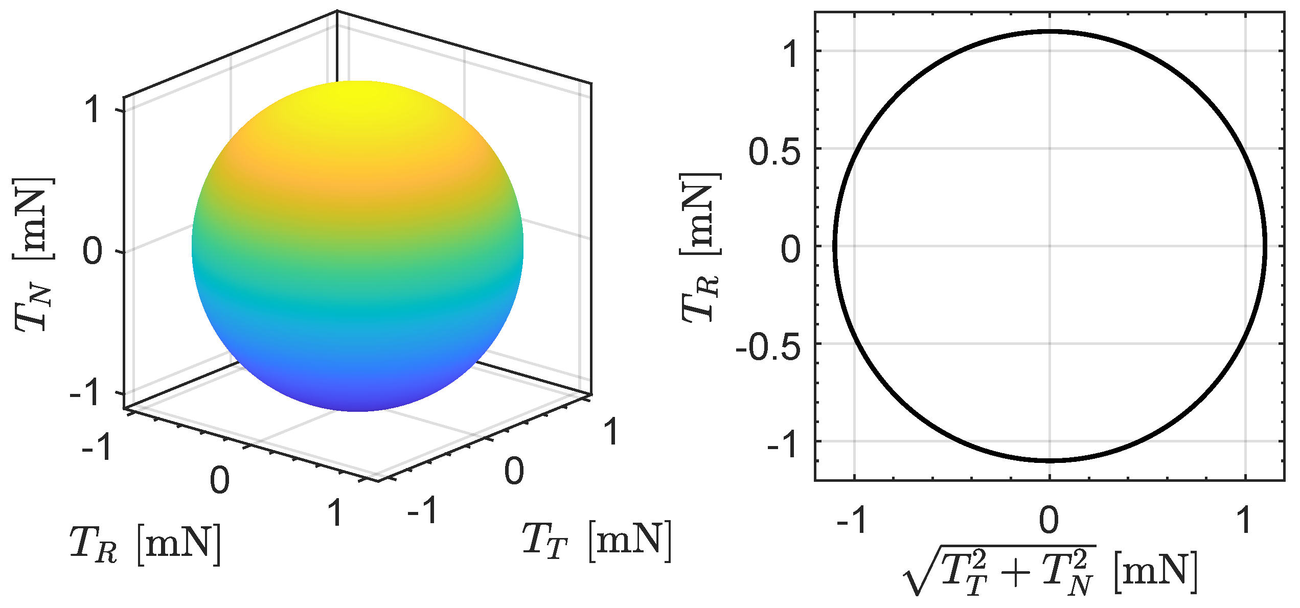
As regards the direction of the thrust vector, which is defined by the unit vector $\widehat{\mathit{T}}$, the usual working hypothesis used in the design of space trajectories based on the use of solar electric propulsion systems is adopted. In particular, it is assumed that the unit vector $\widehat{\mathit{T}}$ is not constrained and that, therefore, the direction of the BIT-3-induced thrust vector $\mathit{T}$ can be oriented in any direction during the flight of the spacecraft. Therefore, the thrust vector can be simply written as

$$\mathit{T}=T \widehat{\mathit{T}}$$

(3)

where value of the thrust magnitude $T=T\left(\mathrm{Id}\right)$ is indicated in Table 3 as a function of the operating level $\mathrm{Id}$. From the point of view of spacecraft dynamics, usually the thrust vector $\mathit{T}$ is more conveniently expressed in a typical radial–transverse–normal reference frame (RTN) whose unit vectors are defined, as a function of the spacecraft position $\mathit{r}$ and velocity $\mathit{v}$ vector, as ${\widehat{\mathit{i}}}_{\mathrm{R}}\triangleq \mathit{r}/\parallel \mathit{r}\parallel$, ${\widehat{\mathit{i}}}_{\mathrm{N}}\triangleq (\mathit{r}\times \mathit{v})/\parallel \mathit{r}\times \mathit{v}\parallel$, ${\widehat{\mathit{i}}}_{\mathrm{T}}\triangleq {\widehat{\mathit{i}}}_{\mathrm{N}}\times {\widehat{\mathit{i}}}_{\mathrm{R}}$. In RTN, the thrust vector is rewritten as

$$\mathit{T}=T_R {\widehat{\mathit{i}}}_{\mathrm{R}}+T_T {\widehat{\mathit{i}}}_{\mathrm{T}}+T_N {\widehat{\mathit{i}}}_{\mathrm{N}}$$

(4)

where $T_R$, $T_T$, and $T_N$ are the radial, transverse, and normal components of the thrust vector, respectively, with $\sqrt{T_R^2+T_T^2+T_N^2}\equiv T\left(\mathrm{Id}\right)$. In the case where the vector $\widehat{\mathit{T}}$ is not constrained, for a given operating level $\mathrm{Id}$, the tip of the thrust vector describes a sphere in the RTN frame. Figure 5 shows such a kind of thrust bubble in the case where the BIT-3 engine unit provides the maximum value of T, that is, in the case of $\mathrm{Id}=5$.

Finally, the thrust model needed to describe the dynamics of the spacecraft includes the differential equation for the total mass variation. Assuming for simplicity that during the flight, the propulsion system is always in TM (i.e., we do not consider the possibility of engaging the SM or the WSM), and taking into account the propellant mass flow rate ${\dot{m}}_p$ given in Table 3, the equation indicating the temporal variation of m is simply the following:

$${\displaystyle \frac{\mathrm{d}m}{\mathrm{d}t}}=-{\dot{m}}_p$$

(5)

where, again, the value of ${\dot{m}}_p$ depends on the selected operating level $\mathrm{Id}$.

Case of Two Engine Units

In this part of the section, we will analyze the case where the CubeSat hosts two identical engine units which are both based on the BIT-3 RF ion thruster (with gimbal) [33]. The total propellant mass stored on board the spacecraft is therefore $2\times 1.5 \mathrm{kg}=3 \mathrm{kg}$, the mass of the combined propulsion system is $2\times 2.9 \mathrm{kg}=5.8 \mathrm{kg}$, and the total occupied volume is $2\times 1.6 \mathrm{U}=3.2 \mathrm{U}$. The interesting case where there are three engine units can be easily modeled by extending the procedure outlined below, while a scenario with four units appears difficult to reconcile with the typical dimensions and weights of CubeSats designed today for scientific applications [50]. In this situation, let us indicate with the subscript ➀ the first of these two identical BIT-3-based engine units, and with the subscript ➁ the remaining unit, so that the symbol ${\mathrm{Id}}_{➀}=[0,1,2,3,4,5]$ (or ${\mathrm{Id}}_{➁}=[0,1,2,3,4,5]$) indicates the thrust level of the first (or the second) engine unit. Let us also assume that each of the two engine units is independent and that therefore its operating level can be selected independently from that of the other unit. This means, among other things, that the electric power input to the PPU of the generic unit can be selected autonomously during the flight.

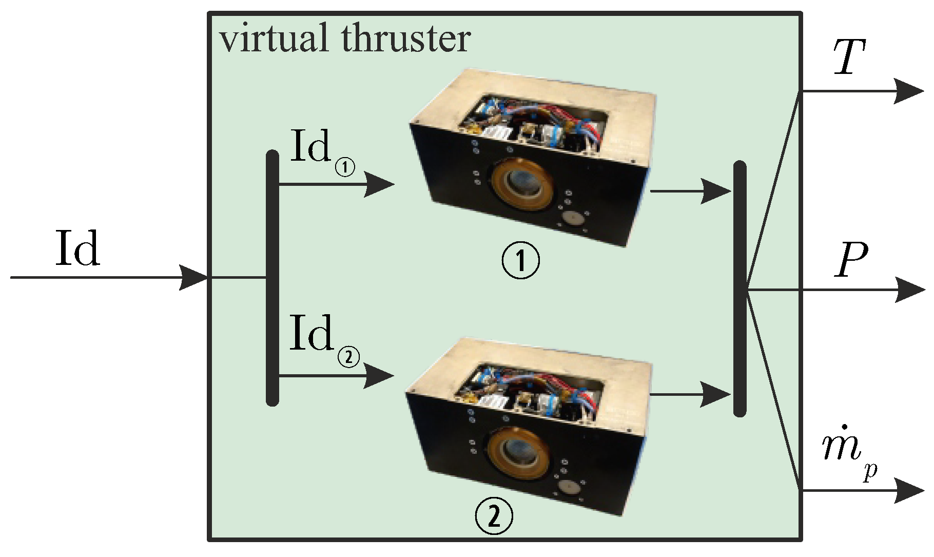
From the point of view of the preliminary design of the spacecraft transfer trajectory, an important aspect to take into account regarding the effect linked to the presence of two engine units is the possibility of having a certain number of different combinations of total thrust magnitude T and total propellant mass flow rate ${\dot{m}}_p$, which obviously correspond to different absorbed (total) electric power levels P. More precisely, in the presence of two independent BIT-3-based engine units, from the point of view of the study of spacecraft dynamics, it is more convenient to consider a sort of virtual propulsion system whose characteristics, in terms of $\{T,{\dot{m}}_p,P\}$, depend on the values chosen for ${\mathrm{Id}}_{➀}$ and ${\mathrm{Id}}_{➁}$, as sketched in Figure 6.

The operating level $\mathrm{Id}$ of such a virtual propulsion system is indicated, as a function of the values of ${\mathrm{Id}}_{➀}$ and ${\mathrm{Id}}_{➁}$, in

Table 4. Operating levels of the virtual propulsion system consisting of two engine units.

	${\mathbf{Id}}_{➀}=0$	${\mathbf{Id}}_{➀}=1$	${\mathbf{Id}}_{➀}=2$	${\mathbf{Id}}_{➀}=3$	${\mathbf{Id}}_{➀}=4$	${\mathbf{Id}}_{➀}=5$
${\mathbf{Id}}_{\mathbf{➁}}=\mathbf{0}$	$\mathrm{Id}=0$	$\mathrm{Id}=1$	$\mathrm{Id}=2$	$\mathrm{Id}=3$	$\mathrm{Id}=4$	$\mathrm{Id}=5$
${\mathbf{Id}}_{\mathbf{➁}}=\mathbf{1}$	—	$\mathrm{Id}=6$	$\mathrm{Id}=7$	$\mathrm{Id}=8$	$\mathrm{Id}=9$	$\mathrm{Id}=10$
${\mathbf{Id}}_{\mathbf{➁}}=\mathbf{2}$	—	—	$\mathrm{Id}=11$	$\mathrm{Id}=12$	$\mathrm{Id}=13$	$\mathrm{Id}=14$
${\mathbf{Id}}_{\mathbf{➁}}=\mathbf{3}$	—	—	—	$\mathrm{Id}=15$	$\mathrm{Id}=16$	$\mathrm{Id}=17$
${\mathbf{Id}}_{\mathbf{➁}}=\mathbf{4}$	—	—	—	—	$\mathrm{Id}=18$	$\mathrm{Id}=19$
${\mathbf{Id}}_{\mathbf{➁}}=\mathbf{5}$	—	—	—	—	—	$\mathrm{Id}=20$

. For example, according to Table 4, the operating level $\mathrm{Id}=0$ is obtained when ${\mathrm{Id}}_{➀}=0$ and ${\mathrm{Id}}_{➁}=0$, so that in this case, bearing in mind the data in Table 3, the total thrust given by the virtual propulsion system is $T=2\times 0.01 \mathrm{mN}=0.02 \mathrm{mN}$, the total propellant mass flow rate is ${\dot{m}}_p=2\times 50.98\mathsf{\mu }\mathrm{g}/\mathrm{s}=101.96\mathsf{\mu }\mathrm{g}/\mathrm{s}$, and the total absorbed electric power is $P=2\times 42 \mathrm{W}=82 \mathrm{W}$. On the other hand, the operating level $\mathrm{Id}=8$ corresponds to a case in which ${\mathrm{Id}}_{➀}=3$ and ${\mathrm{Id}}_{➁}=1$. Accordingly, when $\mathrm{Id}=8$, the total thrust of the virtual engine is $T=0.89 \mathrm{nN}+0.66 \mathrm{nN}=1.55 \mathrm{mN}$, the total propellant mass flow rate is ${\dot{m}}_p=52.15\mathsf{\mu }\mathrm{g}/\mathrm{s}+52.17\mathsf{\mu }\mathrm{g}/\mathrm{s}=104.32\mathsf{\mu }\mathrm{g}/\mathrm{s}$, and the required electric power is $P=65 \mathrm{W}+55 \mathrm{W}=120 \mathrm{W}$.

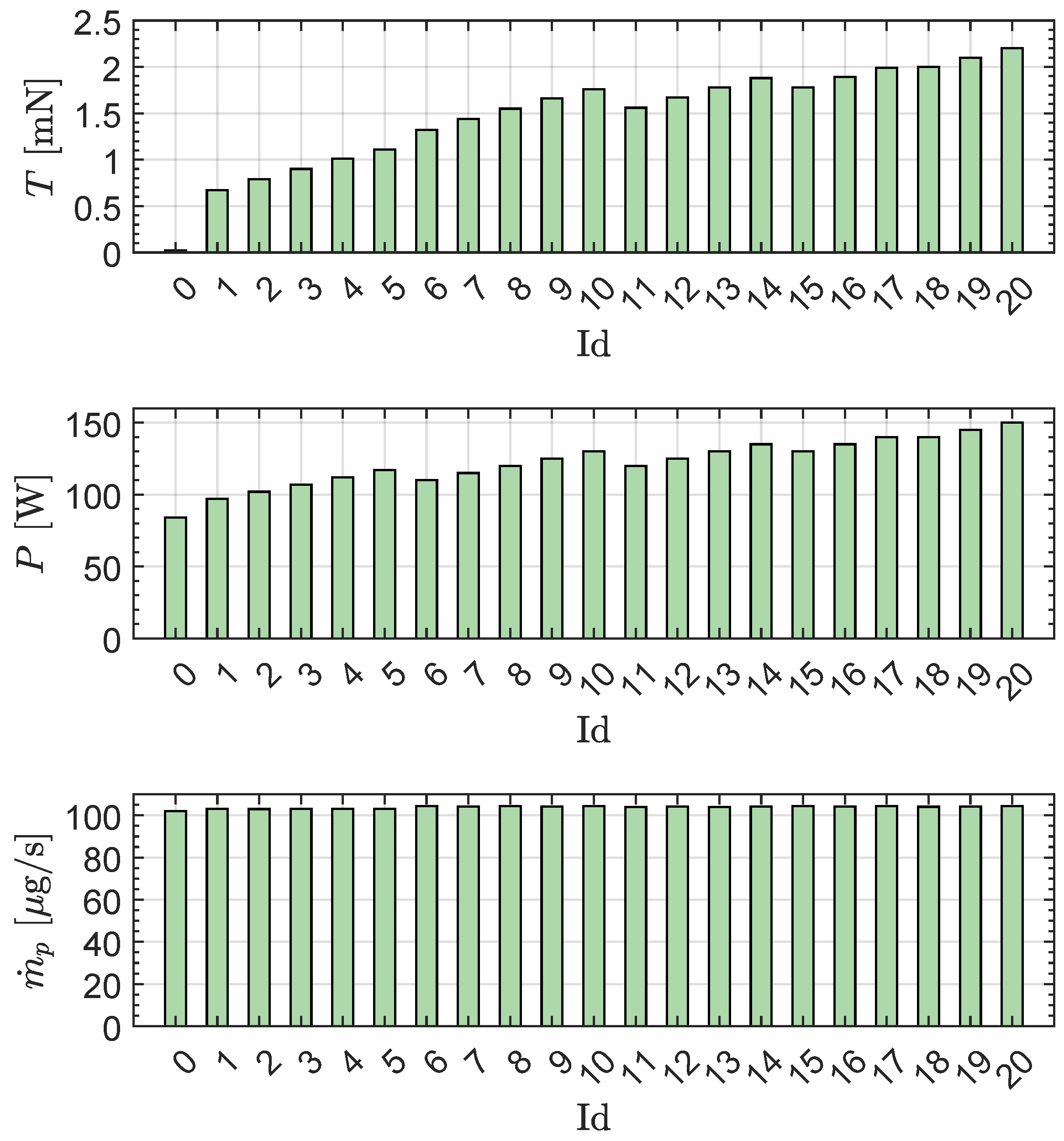
According to the possible combinations of ${\mathrm{Id}}_{➀}$ and ${\mathrm{Id}}_{➁}$ summarized in Table 4, and bearing in mind the data reported in Table 3, one obtains the propulsive performances $\{T,{\dot{m}}_p,P\}$ as a function of the operating level $\mathrm{Id}$ shown in the bar plots of Figure 7. In particular, the figure indicates that the propellant mass flow rate of the propulsion system is roughly $104\mathsf{\mu }\mathrm{g}/\mathrm{s}$ for all the values of $\mathrm{Id}$. The values of $\{T,{\dot{m}}_p,P\}$ for each of the 21 operating levels indicated in Table 4 are also reported in

Table 5. Thrust table of a propulsion system consisting of two identical engine units based on BIT-3.

$\mathbf{Id}$	T [mN]	P [W]	${\dot{\mathit{m}}}_{\mathit{p}}$ [μg/s]
0	$0.02$	84	$101.97$
1	$0.67$	97	$103.15$
2	$0.79$	102	$102.97$
3	$0.90$	107	$103.14$
4	$1.01$	112	$103.01$
5	$1.11$	117	$103.15$
6	$1.32$	110	$104.34$
7	$1.44$	115	$104.15$
8	$1.55$	120	$104.32$
9	$1.66$	125	$104.19$
10	$1.76$	130	$104.34$
11	$1.56$	120	$103.97$
12	$1.67$	125	$104.14$
13	$1.78$	130	$104.01$
14	$1.88$	135	$104.15$
15	$1.78$	130	$104.31$
16	$1.89$	135	$104.18$
17	$1.99$	140	$104.32$
18	$2.00$	140	$104.05$
19	$2.10$	145	$104.19$
20	$2.20$	150	$104.34$

.

3. A Few Notes on the Mathematical Model

This section briefly summarizes the mathematical model used in this work. In particular, the section is divided into three parts. The first part describes the distribution of the CubeSat masses using a simplified approach recently proposed by the author [41] for a small vehicle equipped with a BIT-3-based propulsion system. In particular, this analytical model allows us to schematize the mass breakdown of the typical CubeSat subsystems as a function of the number of engine units installed on board. The second part of the section briefly describes the mathematical model used to study the heliocentric dynamics of the CubeSat in a generally three-dimensional mission scenario. Also in this case, since the equations of motion of a spacecraft equipped with an electric propulsion system have been detailed and commented on several times even in the very recent literature, it is preferable to recall the most suitable references without repeating the model, in order to streamline the discussion. Finally, the last part of the section describes the procedure used to determine the optimal control law during interplanetary transfer by employing an optimization framework.

3.1. Simplified CubeSat Mass Model

The study of the transfer trajectory in a heliocentric mission scenario requires a definition of the CubeSat’s inertia characteristics, which must indicate both the mass $m_0$ of the vehicle at the beginning of the mission (time $t_0\triangleq 0$) and the total mass $m_p$ of the propellant stored on board the CubeSat. The value of the pair $\{m_0,m_p\}$ imposes a constraint on the minimum final mass of the spacecraft, i.e., the total mass of the vehicle at the end of the transfer, which must clearly be greater than the difference $m_0-m_p$. From the point of view of the spacecraft mass distribution, we resort to the simplified analytical mathematical model recently proposed by the author in Ref. [41] to schematize the inertial characteristics of an interplanetary CubeSat equipped with an array of BIT-3-based engine units.

In that simplified model, the spacecraft mass was divided into five components: the dry mass of the engine units $m_e$; the total mass of the propellant $m_p$; the mass of the power generation subsystem $m_{\mathrm{pow}}$; the mass of the payload $m_{\mathrm{pay}}$; and the mass of the remaining subsystems $m_{\mathrm{oth}}$, including the structure and a suitable contingency term. As for the payload, a series of COTS components with a total mass of $m_{\mathrm{pay}}=4 \mathrm{kg}$ are considered, while for the power subsystem, high-efficiency solar arrays such as those made available by MMA [42] are used, with a power-to-mass ratio of $133 \mathrm{W}/\mathrm{kg}$. In particular, the power subsystem was sized to provide the maximum electric power required by the propulsion system and an additional $25 \mathrm{W}$ (required for the operation of the other subsystems, including the scientific payload) up to a solar distance of $1.1 \mathrm{AU}$. Therefore, the electric power $P_{\oplus }$ given by the subsystem at a solar distance of $1 \mathrm{AU}$ is approximatively $P_{\oplus }=(75 \mathrm{W}+25 \mathrm{W})\times 1.1^2\simeq 121 \mathrm{W}$ for the case of a single engine unit, while one has $P_{\oplus }=(2\times 75 \mathrm{W}+25 \mathrm{W})\times 1.1^2\simeq 212 \mathrm{W}$ when there are two engine units; see also the power requirements of a BIT-3-based engine unit summarized in Table 1. According to the procedure described in Ref. [41], when the CubeSat hosts a single engine unit, one has $m_0\simeq 13 \mathrm{kg}$ and $m_p=1.5 \mathrm{kg}$, so the final mass of the vehicle must be greater than $11.5 \mathrm{kg}$. On the other hand, when there are two engine units, the spacecraft initial mass is $m_0\simeq 19 \mathrm{kg}$ and the propellant mass is $m_p=3 \mathrm{kg}$ [41], with a CubeSat’s final mass greater than roughly $16 \mathrm{kg}$. A donut chart of the CubeSat’s mass distribution is reported in Figure 8 as a function of the number of engine units. Note that the mass $m_{\mathrm{oth}}$ is, by assumption, a fixed percentage (i.e., $40\%$) of the total mass $m_0$.

3.2. Spacecraft Heliocentric Dynamics

Following the typical procedure used to complete the preliminary design of the transfer trajectory of an interplanetary spacecraft [16], we consider only the effects related to the gravitational attraction of the Sun and the thrust provided by the solar electric propulsion system. Keeping in mind Equation (5) and observing that the general expression of the thrust vector $\mathit{T}$ induced by BIT-3 is given by Equation (3), while both the thrust magnitude T and propellant mass flow rate ${\dot{m}}_p$ depend on the operating level $\mathrm{Id}$, the CubeSat’s equations of motion are given by the classical relations

$${\displaystyle \frac{\mathrm{d}\mathit{r}}{\mathrm{d}t}}=\mathit{v},{\displaystyle \frac{\mathrm{d}\mathit{v}}{\mathrm{d}t}}=-{\displaystyle \frac{{\mu }_{\odot }}{r^3}}\mathit{r}+{\displaystyle \frac{\mathit{T}}{m}},{\displaystyle \frac{\mathrm{d}m}{\mathrm{d}t}}=-{\dot{m}}_p$$

(6)

where ${\mu }_{\odot }$ is the gravitational parameter of the Sun. The spacecraft dynamics, that is, the seven first-order scalar differential equations which can be derived from Equation (6), can be more conveniently studied by using the set of modified equinoctial elements proposed by Walker [51]. In this case, the equations of motion of the spacecraft become more complex in terms of their writing, but their use in a trajectory calculation routine is simpler than using the Cartesian equations given by the previous relation. The details regarding the use of the modified equinoctial elements [51] and the mathematical form of the spacecraft equations of motion are described in the companion paper [52] to this Special Issue [53], to which the interested reader is referred for further information. In particular, the last of Equation (6) is used, together with Equations (9)–(14) of Ref. [52], in which the three components (radial, transverse, and normal) of the propulsive acceleration vector in RTN are given by the ratios $T_R/m$, $T_T/m$, and $T_N/m$; see also Equation (4).

The initial conditions (i.e., the conditions at time $t_0$) that complete the system of differential Equation (6) model the CubeSat which initially travels in a heliocentric parking orbit that coincides with the orbit of the Earth around the Sun. In this situation, the initial value of m is $m_0$, which is equal to $13 \mathrm{kg}$ in the case of a single engine unit or equal to $19 \mathrm{kg}$ when there are two engine units. The initial value of the spacecraft position and velocity vectors are instead derived from the orbital elements of the Earth’s heliocentric orbit as retrieved from the JPL Horizons On-Line Ephemeris System on the date of 10 April 2025. In particular, the angular position of the CubeSat along the parking orbit is unconstrained and is obtained as the output of the optimization process that provides the heliocentric trajectory of the spacecraft. This optimization process will be briefly described in the next subsection.

3.3. Trajectory Optimization and Optimal Control Laws

The heliocentric trajectory of the CubeSat propelled by BIT-3 was obtained by solving an optimization problem that allows us to study the rapid transfer between the heliocentric (Earth-like) parking orbit and an assigned three-dimensional Keplerian target orbit. The problem studied here is the so-called “orbit-to-orbit” transfer, where the actual ephemerides of the two celestial bodies involved in the transfer are not taken into account, in order to obtain optimal global results in terms of the selected (scalar) performance index. In particular, the optimization process minimizes the flight time required to complete the transfer by also finding the optimal angular position of the spacecraft along both the parking and the target orbits. In this sense, the procedure used in this paper parallels the approach employed in a recent study by the author [54] when the CubeSat is equipped with a hybrid propulsion system given by an electric thruster and a photonic solar sail.

The CubeSat’s trajectory optimization was performed using an indirect approach [55,56], while the optimal control law, in terms of temporal variation of both the direction of the thrust unit vector $\widehat{\mathit{T}}$ and the operating level $\mathrm{Id}$, was obtained by resorting to the PMP [49]. In particular, the optimal control law allows us to maximize the local value of the Hamiltonian function [57] which depends, in addition to the seven state variables (scalars), also on the seven Lagrange multipliers of the problem.

4. Mission Description and Simulation Results

The performance of the BIT-3-propelled CubeSat is studied in an interplanetary mission scenario that includes reaching a near-Earth asteroid. In this context, the heliocentric orbit of object 2000 SG344 was considered, which corresponds to an Aten-class asteroid with a size of just under forty meters. This asteroid has been considered several times in the literature as a possible target for exploration by robotic probes [58,59]. The orbital elements which define the shape and the orientation of the target heliocentric orbit, as obtained by the JPL Horizons On-Line Ephemeris System, are summarized in

Table 6. Orbital elements of the target orbit, that is, the heliocentric orbit of asteroid 2000 SG344.

Orbital Element	Value
semi-major axis	$0.97738 \mathrm{AU}$
eccentricity	$0.06688$
inclination	$0.11308 \mathrm{deg}$
long. of asc. node	$191.7688 \mathrm{deg}$
arg. of perihelion	$275.5316 \mathrm{deg}$

.

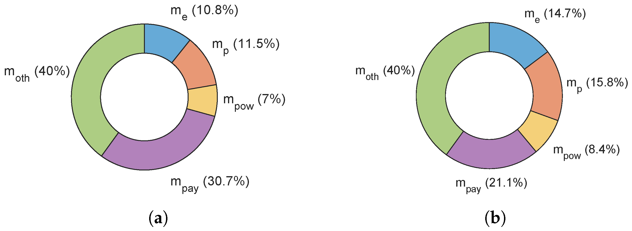
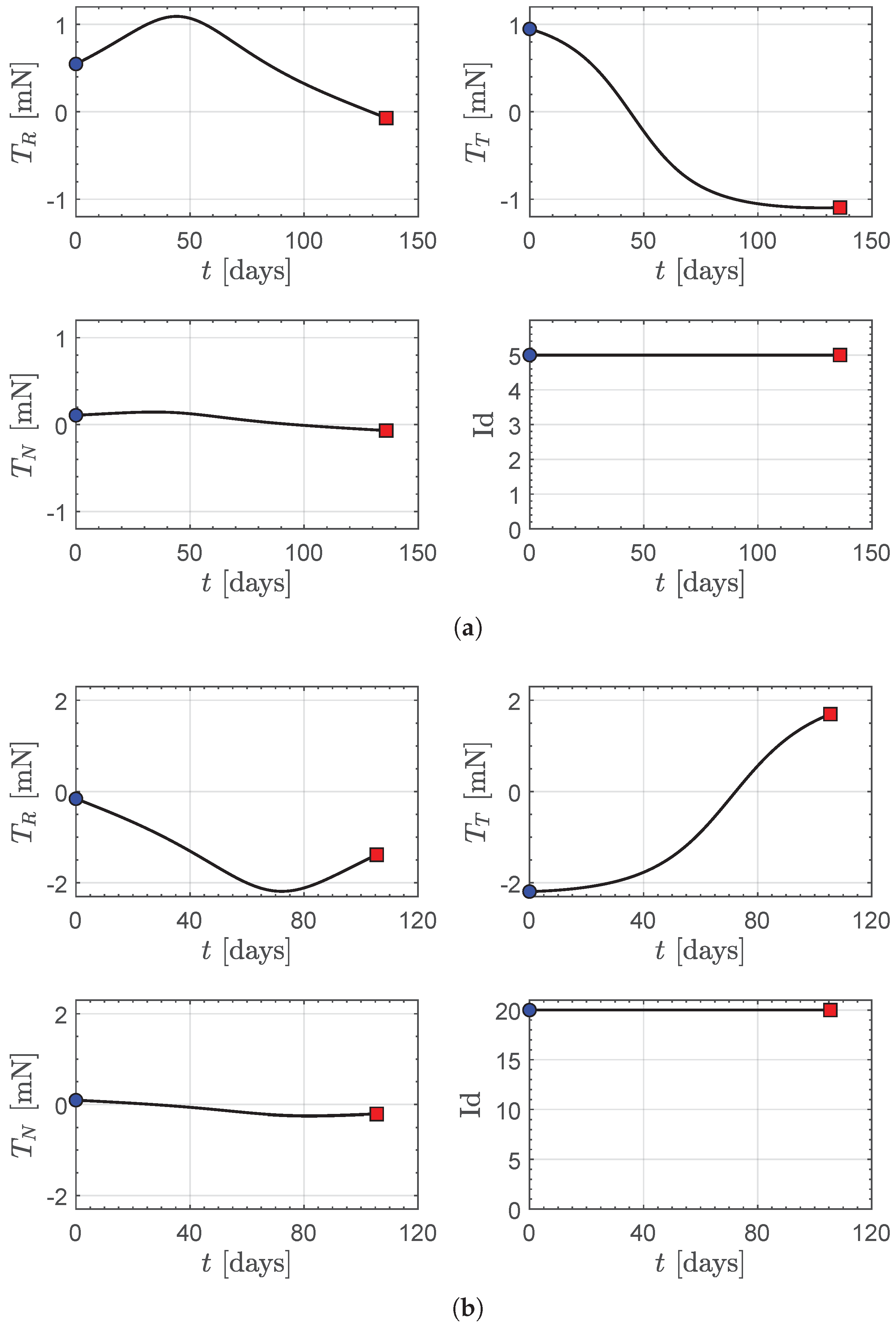
The solution to the optimization problem gives a minimum flight time of about $136 \mathrm{days}$ and a propellant mass expenditure of $0.61 \mathrm{kg}$ (roughly $41\%$ of $m_p$) when the CubeSat hosts a single engine unit, and a transfer time of $105.5 \mathrm{days}$ and a required propellant mass of $0.95 \mathrm{kg}$ (roughly $31\%$ of $m_p$) with two installed engine units. The optimal transfer trajectory of the CubeSat is reported in Figure 9, while Figure 10 shows the temporal variation of the optimal control laws in terms of thrust vector components $\{T_R,T_T,T_N\}$ and operating level $\mathrm{Id}$ as a function of t. In particular, Figure 10 indicates that the propulsion system uses a single operating level during all the transfer, that is, $\mathrm{Id}=5$ when the CubeSat has a single engine unit, and $\mathrm{Id}=20$ when there are two units. In fact, these two operating levels correspond to the maximum magnitude of the thrust vector, as confirmed by Table 3 and Table 5. This is a rather common result when the performance index to be optimized is the flight time and the thrust vector direction is not constrained. Furthermore, the power subsystem is sized to allow the delivery of the required electric power from the maximum thrust level up to a distance from the Sun of $1.1 \mathrm{AU}$, and the optimal transfer trajectory clearly indicates that the spacecraft is at a distance of about $1 \mathrm{AU}$ during the entire heliocentric transfer; see the ecliptic projection of the optimal transfer trajectory shown on the left side of Figure 9. The situation is different when the electric power provided by the solar panels is not sufficient to allow the use of maximum thrust. For this reason, the last part of this section will analyze the transfer to the asteroid 2000 SG344 considering a value of $P_{\oplus }$ smaller than the one that allows obtaining the results summarized in Figure 9 and Figure 10.

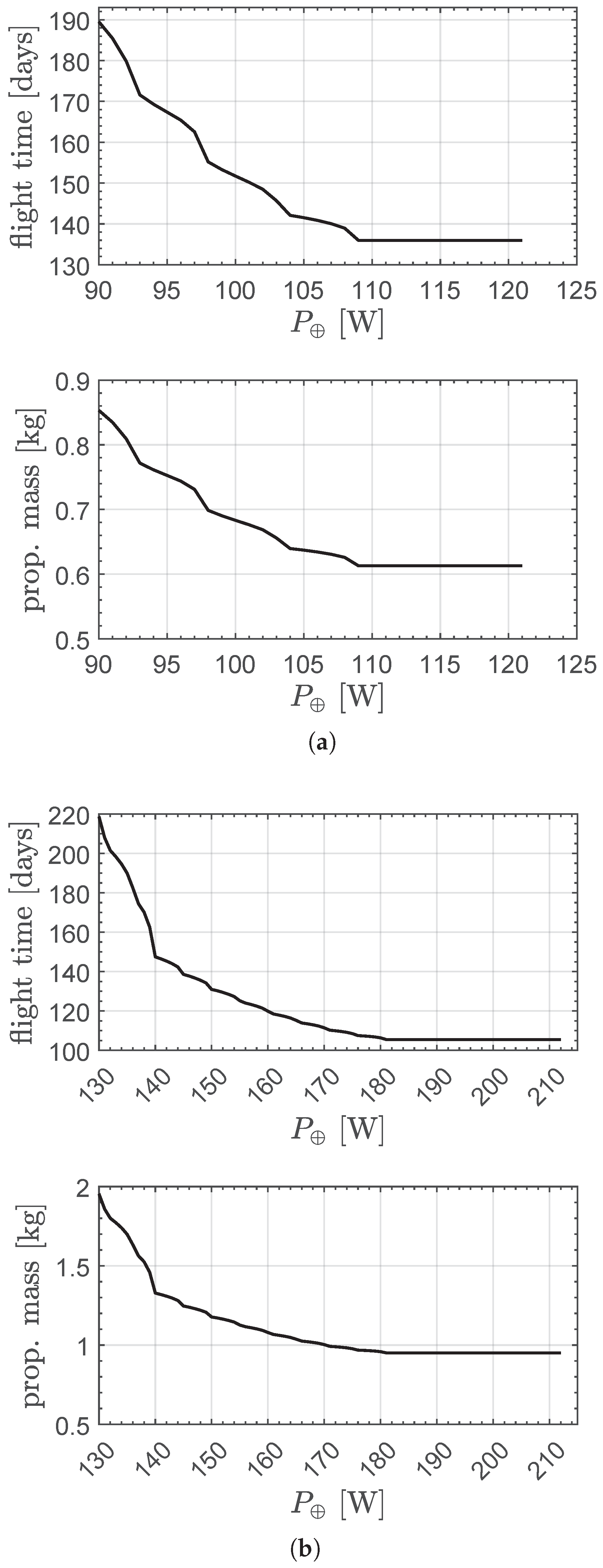
In particular, by solving the optimal control problem several times, a parametric study of the mission performance as a function of the nominal electric power $P_{\oplus }$ was carried out. The results of this specific study, in terms of the minimum flight time and the corresponding propellant mass consumption, are summarized in Figure 11. The figure shows that the transfer performance degrades as the value of $P_{\oplus }$ decreases. For example, in the case of a single engine unit, the transition from $P_{\oplus }=121 \mathrm{W}$ to $P_{\oplus }=90 \mathrm{W}$ results in an increase in flight time of about $60 \mathrm{days}$, while the required propellant mass reaches almost $1 \mathrm{kg}$. This behavior is linked to the fact that the residual electric power (once the remaining on-board subsystems have been powered) is no longer sufficient to allow the activation of the maximum thrust level permitted by the propulsion system. Therefore, other operating levels are used that require a value of electric power compatible with the availability at that given distance from the Sun. These operating levels involve an increase in flight time and a corresponding increase in the propellant mass required to complete the assigned orbital transfer.

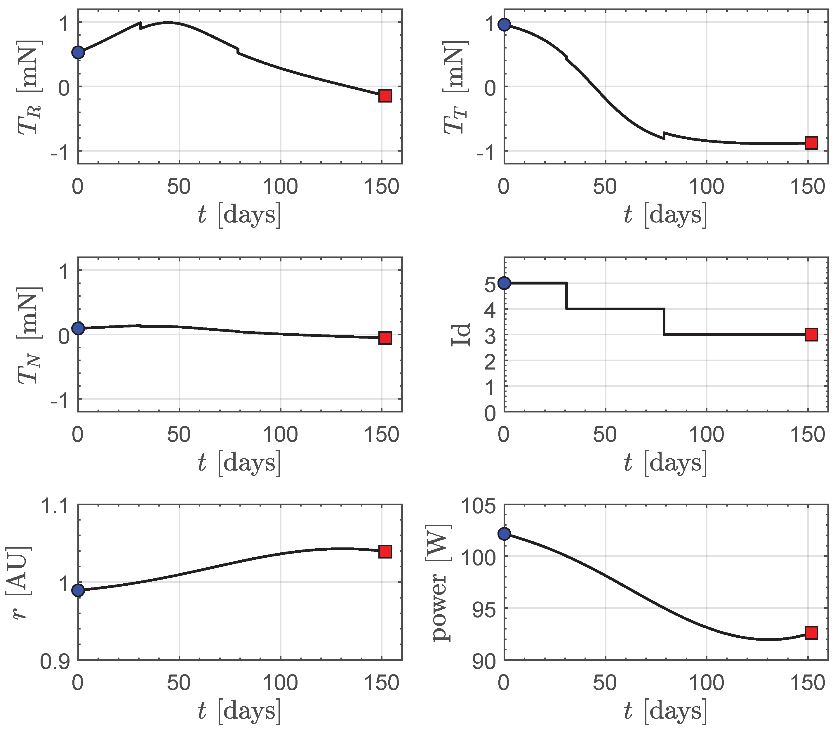
For example, when $P_{\oplus }=100 \mathrm{W}$ and the CubeSat has a single engine unit, the optimal control laws are reported in Figure 12, which shows also the temporal variation of the Sun–spacecraft distance r and the corresponding electric power given by the solar arrays. From Figure 12, we observe that, the engine uses three operating levels during the transfer, while the available electric power drops below $95 \mathrm{W}$ in the second half of the flight. Recall, indeed, that the payload and the other subsystems require an electric power equal to $25 \mathrm{W}$, so that when the available power is $95 \mathrm{W}$ the engine unit can use only a value of $95 \mathrm{W}-25 \mathrm{W}=70 \mathrm{W}$, which is not sufficient to activate the operating level $\mathrm{Id}=5$; see also the last row of Table 1.

5. Final Remarks

This paper has analyzed the performance of a CubeSat equipped with a propulsion system based on the BIT-3 electric thruster in a typical heliocentric scenario involving the transfer between two Keplerian orbits of assigned characteristics. This scenario has been studied in an optimization framework where the flight time required to complete the orbital transfer is minimized. The study of the transfer performance takes into account the actual thrust levels of the engine and also considers the presence of two propulsion units on board, even if the procedure can be easily extended to the case of three units. This possibility of installing two engine units on the CubeSat allows for a large number of possible combinations of thrust and electric power required for the operation of the propulsion system. In particular, in the case in which the electric power is sufficient to activate the operating level corresponding to the maximum available thrust magnitude, and since the direction of the thrust vector is not constrained as often happens in the use of solar electric propulsion systems, the solution of the optimal control problem in which the flight time is minimized provides the classic result where the maximum available thrust value is locally employed. This result corresponds to selecting a single operating level during the entire heliocentric transfer, although the situation is significantly different when the electric power provided by the solar arrays is no longer sufficient to allow the use of any operating level summarized in the engine’s thrust table. In this case, the optimal control law prescribes the use of different thrust levels during the interplanetary flight, depending on the local value of the available electric power. This aspect causes an increase in the flight time and a consequent increase in the propellant mass required for the transfer. One of the assumptions of the mathematical model is related to the fact that the direction of the thrust vector is not constrained during heliocentric flight and, therefore, the thrust can be directed in any direction of space. The presence of a possible constraint on the direction of the thrust vector would lead to a degradation in mission performance.

A lower value of this (required) propellant mass could be obtained by solving an optimization problem in which the final mass of the spacecraft is maximized. The solution to this specific problem, together with the one in which three engine units are considered in the CubeSat preliminary design, is a possible extension of the work illustrated in this paper. A second possible and interesting extension of this work concerns the introduction of a more refined model for the schematization of the electric power supplied by high-performance solar panels. Such a model, for example, could consider the effects related to variations in performances due to the degradation of the film covering the solar cells or to the equilibrium temperature whose value also depends on the distance of the spacecraft from the Sun. A third and last possible completion of the model could concern the analysis of the uncertainties related to the interplanetary trajectory of the spacecraft and therefore, in essence, the possible presence of trajectory correction maneuvers that allow the CubeSat to be brought back along its nominal optimal transfer orbit.

However, although it is theoretically possible to use a continuous-thrust propulsion system, generic trajectory correction maneuvers are planned and implemented assuming a substantially impulsive velocity change, and therefore, a high-thrust propulsion system is used. In this sense, analysis of possible uncertainties in the context of an interplanetary transfer of a small space vehicle such as a CubeSat could then lead to considering an innovative propulsion system capable of providing both (continuous) low thrust with a high specific impulse and (impulsive) high thrust with lower specific impulse. Such a propulsion system could be a hybrid solution between an electric and a chemical engine, or a more innovative thruster that involves the use of a multimode propulsion system in which a single type of propellant is fully exploited with two different thrust concepts.

References

1. Hittepole, P.A.; Hudson, J.S. Guidance for Spacecraft Relative Motion Using Continuous Periodic Thrust. J. Astronaut. Sci. 2025, 72, 4. [Google Scholar] [CrossRef]
2. Lang, X.; de Ruiter, A. Distributed optimal control allocation for 6-dof spacecraft with redundant thrusters. Aerosp. Sci. Technol. 2021, 118, 106971. [Google Scholar] [CrossRef]
3. Wijayatunga, M.C.; Armellin, R.; Holt, H.; Pirovano, L.; Lidtke, A.A. Design and guidance of a multi-active debris removal mission. Astrodynamics 2023, 7, 383–399. [Google Scholar] [CrossRef]
4. Sun, X.; Wang, Y.; Su, J.; Li, J.; Xu, M.; Bai, S. Relative orbit transfer using constant-vector thrust acceleration. Acta Astronaut. 2025, 229, 715–735. [Google Scholar] [CrossRef]
5. Holt, H.; Baresi, N.; Armellin, R. Reinforced Lyapunov controllers for low-thrust lunar transfers. Astrodynamics 2024, 8, 633–656. [Google Scholar] [CrossRef]
6. Fu, B.; Sperber, E.; Eke, F. Solar sail technology—A state of the art review. Prog. Aerosp. Sci. 2016, 86, 1–19. [Google Scholar] [CrossRef]
7. Gong, S.; Macdonald, M. Review on solar sail technology. Astrodynamics 2019, 3, 93–125. [Google Scholar] [CrossRef]
8. Circi, C. Mars and Mercury Missions Using Solar Sails and Solar Electric Propulsion. J. Guid. Control. Dyn. 2004, 27, 496–498. [Google Scholar] [CrossRef]
9. Janhunen, P. Electric sail for spacecraft propulsion. J. Propuls. Power 2004, 20, 763–764. [Google Scholar] [CrossRef]
10. Janhunen, P.; Sandroos, A. Simulation study of solar wind push on a charged wire: Basis of solar wind electric sail propulsion. Ann. Geophys. 2007, 25, 755–767. [Google Scholar] [CrossRef]
11. Mengali, G.; Quarta, A.A.; Janhunen, P. Considerations of electric sailcraft trajectory design. JBIS-J. Br. Interplanet. Soc. 2008, 61, 326–329. [Google Scholar]
12. Bassetto, M.; Niccolai, L.; Quarta, A.A.; Mengali, G. A comprehensive review of Electric Solar Wind Sail concept and its applications. Prog. Aerosp. Sci. 2022, 128, 100768. [Google Scholar] [CrossRef]
13. Brophy, J.R.; Noca, M. Electric Propulsion for Solar System Exploration. J. Propuls. Power 1998, 14, 700–707. [Google Scholar] [CrossRef]
14. Brophy, J.R. Perspectives on the success of electric propulsion. J. Electr. Propuls. 2022, 1, 9. [Google Scholar] [CrossRef]
15. Casanova-Álvarez, M.; Navarro-Medina, F.; Tommasini, D. Feasibility study of a Solar Electric Propulsion mission to Mars. Acta Astronaut. 2024, 216, 129–142. [Google Scholar] [CrossRef]
16. Rayman, M.D.; Williams, S.N. Design of the First Interplanetary Solar Electric Propulsion Mission. J. Spacecr. Rocket. 2002, 39, 589–595. [Google Scholar] [CrossRef]
17. Rayman, M.D.; Varghese, P.; Lehman, D.H.; Livesay, L.L. Results from the Deep Space 1 technology validation mission. Acta Astronaut. 2000, 47, 475–487. [Google Scholar] [CrossRef]
18. Rayman, M.D. The successful conclusion of the Deep Space 1 mission: Important results without a flashy title. Space Technol. 2003, 23, 185–196. [Google Scholar]
19. Sengupta, A.; Anderson, J.A.; Gamer, C.; Brophy, J.R.; De Groh, K.K.; Banks, B.A.; Thomas, T.A.K. Deep space 1 flight spare ion thruster 30,000-hour life test. J. Propuls. Power 2009, 25, 105–117. [Google Scholar] [CrossRef]
20. Morris, T.; Jugroot, M. Study of an electrostatic micropropulsion system for nanosatellites. Can. Aeronaut. Space J. 2011, 57, 99–105. [Google Scholar] [CrossRef]
21. Seifert, B.; Bettiol, L.; Buldrini, N.; Eizinger, M.; Krejci, D.; Del Amo, J.G.; Massotti, L. Field Emission Electric Propulsion: Enabling future Science and Earth Observation Missions. In Proceedings of the 2024 IEEE Aerospace Conference, Big Sky, MT, USA, 2–9 March 2024. [Google Scholar] [CrossRef]
22. Asher, J.; Acarregui, O.; Wang, J. Numerical Simulation of Ionic Electrospray Contamination for Small Satellite Formation Flight. IEEE Trans. Plasma Sci. 2023, 51, 2508–2514. [Google Scholar] [CrossRef]
23. Burroni, T.; Thangavel, K.; Servidia, P.; Sabatini, R. Distributed satellite system autonomous orbital control with recursive filtering. Aerosp. Sci. Technol. 2024, 145, 108859. [Google Scholar] [CrossRef]
24. Mahfouz, A.; Gaias, G.; Dalla Vedova, F.; Voos, H. Low-thrust under-actuated satellite formation guidance and control strategies. Acta Astronaut. 2025, 232, 405–423. [Google Scholar] [CrossRef]
25. Kabirov, V.; Semenov, V.; Torgaeva, D.; Otto, A. Miniaturization of spacecraft electrical power systems with solar-hydrogen power supply system. Int. J. Hydrog. Energy 2023, 48, 9057–9070. [Google Scholar] [CrossRef]
26. Fountain, G.H.; Weaver, H.A.; Reuter, D.C.; Stern, S.A.; Linscott, I.R.; McComas, D.J.; Hill, M.E.; Horányi, M. The New Horizons Instrument Suite. Johns Hopkins APL Tech. Dig. (Applied Phys. Lab.) 2023, 37, 34–48. [Google Scholar]
27. Gosain, S.; Harvey, J.; Martinez Pillet, V.; Hill, F.; Woods, T.N. A Compact Full-disk Solar Magnetograph Based on Miniaturization of the GONG Instrument. Publ. Astron. Soc. Pac. 2023, 135, 045001. [Google Scholar] [CrossRef]
28. Alnaqbi, S.; Darfilal, D.; Swei, S.S.M. Propulsion Technologies for CubeSats: Review. Aerospace 2024, 11, 502. [Google Scholar] [CrossRef]
29. Heaton, A.; Miller, K.; Ahmad, N. Near Earth asteroid Scout solar sail thrust and torque model. In Proceedings of the 4th International Symposium on Solar Sailing (ISSS 2017), Kyoyo, Japan, 17–20 January 2017. [Google Scholar]
30. Johnson, L.; Castillo-Rogez, J.; Lockett, T. Near Earth asteroid Scout: Exploring asteroid 1991VG using a Smallsat. In Proceedings of the 70th International Astronautical Congress, Washington, DC, USA, 21–25 October 2019. [Google Scholar]
31. Lockett, T.R.; Castillo-Rogez, J.; Johnson, L.; Matus, J.; Lightholder, J.; Marinan, A.; Few, A. Near-Earth Asteroid Scout Flight Mission. IEEE Aerosp. Electron. Syst. Mag. 2020, 35, 20–29. [Google Scholar] [CrossRef]
32. O’Reilly, D.; Herdrich, G.; Kavanagh, D.F. Electric Propulsion Methods for Small Satellites: A Review. Aerospace 2021, 8, 22. [Google Scholar] [CrossRef]
33. Busek Co. Inc. BIT-3: Compact and Efficient Iodine Gridded Ion Thruster. 2025. Available online: https://www.busek.com/bit3 (accessed on 6 April 2025).
34. Tsay, M.; Frongillo, J.; Model, J.; Zwahlen, J.; Paritsky, L. Maturation of iodine-fueled BIT-3 RF ion thruster and RF neutralizer. In Proceedings of the 52nd AIAA/SAE/ASEE Joint Propulsion Conference, Salt Lake City, UT, USA, 25–27 July 2016. [Google Scholar] [CrossRef]
35. Tsay, M.; Frongillo, J.; Model, J.; Zwahlen, J.; Barcroft, C.; Feng, C. Neutralization demo and thrust stand measurement for BIT-3 RF ion thruster. In Proceedings of the 53rd AIAA/SAE/ASEE Joint Propulsion Conference, Atlanta, GA, USA, 10–12 July 2017. [Google Scholar] [CrossRef]
36. Tsay, M.; Model, J.; Barcroft, C.; Frongillo, J. Integrated Testing of Iodine BIT-3 RF Ion Propulsion System for 6U CubeSat Applications. In Proceedings of the 35th International Electric Propulsion Conference, Atlanta, GA, USA, 8–12 October 2017. [Google Scholar]
37. Babuscia, A.; Hardgrove, C.; Cheung, K.M.; Scowen, P.; Crowell, J. Telecommunication system design for interplanetary CubeSat missions: LunaH-Map. In Proceedings of the IEEE Aerospace Conference Proceedings, Big Sky, MT, USA, 4–11 March 2017. [Google Scholar] [CrossRef]
38. Bosanac, N.; Cox, A.D.; Howell, K.C.; Folta, D.C. Trajectory design for a cislunar CubeSat leveraging dynamical systems techniques: The Lunar IceCube mission. Acta Astronaut. 2018, 144, 283–296. [Google Scholar] [CrossRef]
39. Englander, J.A.; Folta, D.C.; Hur-Diaz, S.H. Optimization of the Lunar Icecube Trajectory Using Stochastic Global Search and Multi-Point Shooting. In Proceedings of the AAS/AIAA Astrodynamics Specialist Meeting, Virtual Event, 9–13 August 2020. [Google Scholar]
40. Quarta, A.A. Exploration of Earth’s Magnetosphere Using CubeSats with Electric Propulsion. Aerospace 2025, 12, 211. [Google Scholar] [CrossRef]
41. Quarta, A.A. Preliminary Trajectory Analysis of CubeSats with Electric Thrusters in Nodal Flyby Missions for Asteroid Exploration. Remote Sens. 2025, 17, 513. [Google Scholar] [CrossRef]
42. MMA Space. MMA HaWK Solar Arrays. 2025. Available online: https://mmadesignllc.com/next-gen-solar-arrays/ (accessed on 6 April 2025).
43. Tsay, M.; Terhaar, R.; Emmi, K.; Barcroft, C. Volume Production of Gen-2 Iodine BIT-3 Ion Propulsion System. In Proceedings of the 37th International Electric Propulsion Conference, Cambridge, MA, USA, 19–23 June 2022. [Google Scholar]
44. Tsay, M. 3,500–Hour Wear Test Result of BIT-3 RF Ion Propulsion System. In Proceedings of the 37th International Electric Propulsion Conference, Cambridge, MA, USA, 19–23 June 2022. [Google Scholar]
45. De Grossi, F.; Carbone, A.; Spiller, D.; Ottaviani, D.; Mengoni, R.; Circi, C. Transcription and optimization of an interplanetary trajectory through quantum annealing. Astrodynamics 2025, 9, 195–215. [Google Scholar] [CrossRef]
46. Bell, D.J. Optimal Space Trajectories—A Review of Published Work. Aeronaut. J. 1968, 72, 141–146. [Google Scholar] [CrossRef]
47. Betts, J.T. Survey of Numerical Methods for Trajectory Optimization. J. Guid. Control Dyn. 1998, 21, 193–207. [Google Scholar] [CrossRef]
48. Chai, R.; Savvaris, A.; Tsourdos, A.; Chai, S.; Xia, Y. A review of optimization techniques in spacecraft flight trajectory design. Prog. Aerosp. Sci. 2019, 109, 100543. [Google Scholar] [CrossRef]
49. Ross, I.M. A Primer on Pontryagin’s Principle in Optimal Control; Collegiate Publishers: San Francisco, CA, USA, 2015; Chapter 2; pp. 127–129. [Google Scholar]
50. Francisco, C.; Henriques, R.; Barbosa, S. A Review on CubeSat Missions for Ionospheric Science. Aerospace 2023, 10, 622. [Google Scholar] [CrossRef]
51. Walker, M.J.H. Erratum: A set of modified equinoctial orbit elements. Celest. Mech. 1986, 38, 391–392. [Google Scholar] [CrossRef]
52. Bassetto, M.; Mengali, G.; Quarta, A.A. Deterministic trajectory design and attitude maneuvers of gradient-index solar sail in interplanetary transfers. Appl. Sci. 2024, 14, 10463. [Google Scholar] [CrossRef]
53. Hu, W.; Hsiao, F. Advances in Spacecraft Attitude and Orbital Dynamics, Control, Trajectory Planning and Navigation. 2025. Available online: https://www.mdpi.com/journal/applsci/special_issues/OJ99GSBF73 (accessed on 13 April 2025).
54. Quarta, A.A. Thrust model and trajectory design of an interplanetary CubeSat with a hybrid propulsion system. Actuators 2024, 13, 384. [Google Scholar] [CrossRef]
55. Quarta, A.A. Initial costate approximation for rapid orbit raising with very low propulsive acceleration. Appl. Sci. 2024, 14, 1124. [Google Scholar] [CrossRef]
56. Quarta, A.A. Three-dimensional guidance laws for spacecraft propelled by a SWIFT propulsion system. Appl. Sci. 2024, 14, 5944. [Google Scholar] [CrossRef]
57. Stengel, R.F. Optimal Control and Estimation; Dover Books on Mathematics; Dover Publications, Inc.: New York, NY, USA, 1994; pp. 222–254. ISBN 978-0486682006. [Google Scholar]
58. Caliskan, G.; Karatas, Y.; Newman, B. Near Earth asteroid mission design for 2000 SG344. In Proceedings of the 6th International Conference on Recent Advances in Space Technologies, Istanbul, Turkey, 12–14 June 2013. [Google Scholar] [CrossRef]
59. García Yárnoz, D.; Sanchez, J.P.; McInnes, C.R. Easily retrievable objects among the NEO population. Celest. Mech. Dyn. Astron. 2013, 116, 367–388. [Google Scholar] [CrossRef]
Figure 1. The picture shows a cutaway of the Busek’s BIT-3 RF ion thruster with a two-axis (optional) gimbal system. The volume of the engine unit is 1.6 U, the dry mass with gimbal is 1.4 kg, and the mass of the stored (solid iodine) propellant is 1.5 kg. This picture has also been included in the author’s recent work [40] to illustrate this miniaturized electric propulsion system. Image courtesy of Busek Co. Inc., Natick, MA, USA.
Applsci 15 06314 g001
Figure 2. Propulsive characteristics { T , P , I sp , C } of the BIT-3 engine unit as a function of the operating level Id = [ 0 , 1 , 2 , 3 , 4 , 5 ] . Data retrieved from Ref. [44] and detailed in Table 1.
Applsci 15 06314 g002
Figure 3. Linear variation in the thrust magnitude T as a function of the screen grid current C as described by Equation (1). Black line → analytical approximation; green dot → actual values given by Table 1.
Applsci 15 06314 g003
Figure 4. Bar plot of the propellant mass flow rate as a function of the engine unit’s operating level.
Applsci 15 06314 g004
Figure 5. Thrust bubble when the operating level is Id = 5 and the engine unit gives the maximum thrust magnitude of 1.1   mN .
Applsci 15 06314 g005
Figure 6. Conceptual sketch of the virtual propulsion system given by two engine units based on the BIT-3 RF ion thruster.
Applsci 15 06314 g006
Figure 7. Propulsive performances, in terms of total thrust T, total propellant mass flow rate m ˙ p , and the resulting adsorbed power P, as a function of the operating level Id of a propulsion system consisting of two identical engine units based on BIT-3.
Applsci 15 06314 g007
Figure 8. Mass distribution of the CubeSat with a payload mass of 4   kg as a function of the number of engine units. (a) Case of a single engine unit with m 0 13   kg ; (b) case of two engine units with m 0 19   kg .
Applsci 15 06314 g008
Figure 9. Optimal CubeSat three-dimensional transfer trajectory (right side) and its ecliptic projection (left side). The scale of the z axis in the graph on the right is exaggerated to better visualize the three-dimensionality of the mission scenario. Black line → CubeSat trajectory; blue line → Earth’s orbit; red line → asteroid’s orbit; star → perihelion point; blue dot → starting point; red square → arrival point; orange circle → the Sun. (a) Case of a single engine unit; (b) case of two engine units.
Applsci 15 06314 g009
Figure 10. Optimal control laws as a function of the number of engine units. Blue dot → start; red square → arrival. (a) Case of a single engine unit; (b) case of two engine units.
Applsci 15 06314 g010
Figure 11. Optimal flight time and propellant mass consumption as a function of the electric power at a distance of 1   AU from the Sun. (a) Case of a single engine unit; (b) case of two engine units.
Applsci 15 06314 g011
Figure 12. Optimal control laws when P = 100   W and the CubeSat has a single engine unit. Blue dot → start; red square → arrival.
Applsci 15 06314 g012