AI-Driven Predictive Maintenance for Workforce and Service Optimization in the Automotive Sector

Abstract

Vehicle owners often use certified service centers throughout the warranty period, which usually extends for five years after buying. Nonetheless, after this timeframe concludes, a large number of owners turn to unapproved service providers, mainly motivated by financial factors. This change signifies a significant drop in income for automakers and their certified service networks. To tackle this issue, manufacturers utilize customer relationship management (CRM) strategies to enhance customer loyalty, usually depending on segmentation methods to pinpoint potential clients. However, conventional approaches frequently do not successfully forecast which clients are most likely to need or utilize maintenance services. This research introduces a machine learning-driven framework aimed at forecasting the probability of monthly maintenance attendance for customers by utilizing an extensive historical dataset that includes information about both customers and vehicles. Additionally, this predictive approach supports workforce planning and scheduling within after-sales service centers, aligning with AI-driven labor optimization frameworks such as those explored in the AI4LABOUR project. Four algorithms in machine learning—Decision Tree, Random Forest, LightGBM (LGBM), and Extreme Gradient Boosting (XGBoost)—were assessed for their forecasting capabilities. Of these, XGBoost showed greater accuracy and reliability in recognizing high-probability customers. In this study, we propose a machine learning framework to predict vehicle maintenance visits for after-sales services, leading to significant operational improvements. Furthermore, the integration of AI-driven workforce allocation strategies, as studied within the AI4LABOUR (reshaping labor force participation with artificial intelligence) project, has contributed to more efficient service personnel deployment, reducing idle time and improving customer experience. By implementing this approach, we achieved a 20% reduction in information delivery times during service operations. Additionally, survey completion times were reduced from 5 min to 4 min per survey, resulting in total time savings of approximately 5906 h by May 2024. The enhanced service appointment scheduling, combined with timely vehicle maintenance, also contributed to reducing potential accident risks. Moreover, the transition from a rule-based maintenance prediction system to a machine learning approach improved efficiency and accuracy. As a result of this transition, individual customer service visit rates increased by 30%, while corporate customer visits rose by 37%. This study contributes to ongoing research on AI-driven workforce planning and service optimization, particularly within the scope of the AI4LABOUR project.

1. Introduction

After-sales service for high-value equipment is a key element of competitive strategy, with manufacturers offering warranties that provide maintenance services from authorized centers. However, after the warranty expires, many asset owners shift to lower-cost, unauthorized service centers, impacting long-term revenue and customer loyalty. Kumar et al.’s research shows that while 84% of vehicles stay loyal to authorized centers within the first year of the warranty, this figure plummets to 29% in the second year, highlighting significant revenue loss and market share erosion for manufacturers. Customer retention is critical, as acquiring new customers is five times more costly than retaining existing ones. Despite substantial investments in CRM programs across industries, many organizations still use simple, rule-based segmentation methods, which fail to capture the complexity of customer behavior, leading to inefficiencies and inaccurate predictions.

In the automotive after-sales domain, customer retention presents a particularly underexplored challenge. While substantial research has been devoted to general customer retention, the specific intersection of vehicle usage patterns and customer behavior within the after-sales service sector remains relatively untapped. This paper aims to address this gap by leveraging advanced machine learning techniques to predict future service visits with high accuracy, enhancing decision-making in the management of after-sales services. Unlike existing studies that primarily focus on fault detection or generalized customer churn, our approach integrates both maintenance demand forecasting and customer behavior analysis in a way that accounts for the complex interplay of these factors.

To this end, we propose a novel machine learning framework tailored for the prediction of vehicle visits to authorized service centers within a predefined period. The model employs several tree-based algorithms—Decision Trees, Random Forests, Light Gradient Boosting Machine (LGBM), and Extreme Gradient Boosting (XGBoost)—to capture the intricate relationships between customer behaviors and maintenance needs. These algorithms were specifically selected for their ability to handle complex datasets and to provide statistically interpretable results. Among these models, XGBoost demonstrated the best performance, showcasing its potential in solving real-world business problems.

By implementing this machine learning framework, we have achieved several key operational improvements. Information delivery times during service operations have been reduced by 20%, and survey completion times have decreased from 5 min to 4 min per survey, resulting in total time savings of approximately 5906 h by May 2024. Moreover, timely vehicle maintenance and service appointment scheduling have contributed to reducing potential accidents. The transition from a rule-based maintenance prediction system to machine learning has also led to better resource utilization and increased prediction accuracy. As a result, individual customer service visit rates have increased by 30%, while corporate customer visits have risen by 37%, highlighting the significant impact of this approach on both customer retention and service efficiency. This framework has the potential to be widely adopted across the automotive industry as a scalable and effective solution for optimizing after-sales service operations. Its machine learning-driven approach can be easily customized and extended to accommodate diverse vehicle brands, models, and customer segments, making it applicable to various contexts within the automotive sector.

This study is motivated by the challenges faced by the after-sales services (ASS) department of a distributor for a German automotive brand in Turkey, which currently utilizes a costly and inefficient rule-based system to predict customer visits. The existing system relies on historical visit data and attempts to predict future service visits by contacting customers who are most likely to visit within a year. However, this approach is problematic as customer behaviors can vary significantly due to factors such as economic conditions, social trends, and external events like the COVID-19 pandemic. Moreover, the previous system was entirely dependent on human effort, where identifying potential customer-vehicle visits required rule-based filtering and weeks of manual analysis. This labor-intensive process not only led to inefficiencies but also limited scalability and adaptability. By integrating AI-driven methodologies, particularly through AI4LABOUR (reshaping labor force participation with artificial intelligence), we have transformed this process into an automated, data-driven system, significantly reducing the time and effort required while improving prediction accuracy and operational efficiency. This study aligns with AI-driven workforce optimization efforts, such as those explored in the AI4LABOUR project, to enhance efficiency in after-sales service management.

Machine learning and artificial intelligence (AI) offer promising solutions to these challenges by enabling more precise demand forecasts, optimized customer segmentation, and improved resource management. By incorporating advanced AI techniques, businesses can reduce costs and enhance the efficiency of their after-sales operations, leading to higher customer retention rates and better overall service outcomes.

The dataset utilized in this study spans over a decade of maintenance records for a diverse set of vehicles, providing a rich foundation for training machine learning models. This comprehensive dataset is carefully preprocessed to derive meaningful features such as service interval patterns, vehicle age, and service fee increases, ensuring that the resulting models are both robust and accurate in predicting future service visits.

The key contributions of this paper are as follows:

I.

Novel Use Case: We present a unique approach to predictive maintenance by focusing on forecasting service visits within the automotive after-sales domain. This framework provides valuable insights for future studies in the area of maintenance demand forecasting.

II.

Enriched Feature Set: We develop and analyze a set of features that significantly improve the predictive accuracy of our models, including patterns in service intervals, vehicle age dynamics, and customer segmentation based on service behaviors.

III.

Machine Learning Comparison: Through a comparative evaluation of four different tree-based algorithms, we identify XGBoost as the most effective model for this particular application, outperforming other methods in terms of predictive accuracy and scalability.

IV.

Practical Implications for CRM and Workforce Planning: The findings of this study offer valuable, actionable insights for CRM teams by enabling the optimization of customer outreach strategies, minimizing resource inefficiencies, and enhancing customer engagement through personalized communication channels such as text messages, emails, and phone calls. Moreover, beyond its immediate application in predictive maintenance, the machine learning approach adopted in this research aligns with the broader objectives of the AI4LABOUR project, particularly in the context of workforce analytics and planning. By leveraging AI to anticipate service demand fluctuations, the underlying methodology demonstrates strong potential for adaptation to labor market forecasting—empowering organizations and policymakers to identify emerging skill gaps, respond proactively to workforce transitions, and support more efficient workforce participation strategies.

The remainder of the paper is organized as follows: Section 2 provides a comprehensive review of related works. Section 3 details the dataset used, including data collection methods and exploratory analysis. Section 4 outlines the methodology employed in this study, including performance evaluation metrics. Section 5 presents the experimental results and analysis. Section 6 concludes the paper with a discussion on the implications of the findings and directions for future research.

2. Related Works

The relevant literature for this study includes research on customer retention and predictive maintenance (PdM). The related studies are summarized below in Section 2.1, Section 2.2 and Section 2.3.

2.1. Customer Retention Studies

Customer retention is a critical aspect of the automotive industry’s business model, with AI technologies playing a pivotal role in enhancing customer engagement and loyalty. While it is commonly assumed that retaining a customer is significantly more cost-effective than acquiring a new one, recent work [1] emphasizes that this assumption must be evaluated through the lens of marginal versus average costs. From this perspective, firms are advised to align retention and acquisition spending with expected customer lifetime value, reinforcing the importance of data-driven strategies in customer relationship management. In this context, AI-based models not only support churn prediction and personalized marketing but also enable dynamic resource allocation for customer retention efforts. Recent industry research highlights the growing organizational investment in CRM systems as part of broader customer retention strategies. According to a large-scale CRM implementation report [2], companies spend an average of 11 weeks selecting a CRM, with nearly 48% of employees using the system once deployed. The average cost per user is estimated at USD 7500 over a five-year period. Most firms cited “supporting business growth” as the leading motivation for CRM adoption, suggesting that CRM platforms are increasingly viewed as strategic assets rather than mere data repositories.

Although AI applications in customer service are widely adopted to enhance efficiency and customer retention, some implementations may carry hidden risks that undermine their intended value. One recent study [3] proposes a framework to diagnose the value-destruction potential of AI and machine learning systems within business processes. The study highlights how flaws in input data, model logic, or system outputs can compromise the effectiveness of AI-based tools such as customer service chatbots. These risks can lead to diminished service quality, customer dissatisfaction, and ultimately reduced loyalty—directly contradicting the strategic goals of retention-focused AI deployments. A customer churn prediction model utilizing unstructured data from telephone communications is proposed in [4]. This study explores customer loyalty through call center data, employing various text mining techniques to analyze clients’ call logs. The churn models developed can predict churn risks with high accuracy and provide meaningful insights.

In the broader telecommunications domain, related models offer methodological insights that can inspire solutions in the automotive context.

In [5], experiments are conducted to enhance the predictive ability of churn models in the context of a personal phone service system. The findings show that the developed churn model performs well, even with an imbalanced class distribution and limited customer data.

In [6], the authors present a comparative study of the most widely used machine learning methods for addressing the customer churn problem in the telecommunications industry. Among various classification techniques, such as Artificial Neural Networks (ANNs), Support Vector Machines (SVMs), Decision Tree (DT), Naive Bayes (NB), and logistic regression (LR), the SVM-POLY model using AdaBoost is identified as the most effective, achieving an accuracy of nearly 97% and an F1-score exceeding 84%.

Such performance benchmarks inform model selection processes in automotive churn prediction problems, especially in environments with high dimensionality and class imbalance.

Similarly, ref. [7] investigates the combination of two neural network methods—backpropagation ANN and Self-Organizing Maps (SOMs)—for predicting customer churn. These hybrid models outperform single neural network models in terms of prediction accuracy and the reduction in Type I and Type II errors across three test sets.

In [8], ANN and DT are applied to identify lost customers in the automotive supplier industry, with results indicating that while both algorithms are efficient, Decision Trees are complicated by the need for buck tuning in loss detection.

The above studies collectively demonstrate that hybrid and ensemble methods often outperform standalone models, particularly when dealing with non-linear and high-noise datasets.

Ref. [9] provides an empirical analysis of the impact of hyperparameters on churn prediction using Deep Neural Networks (DNNs) in the banking industry. The DNN model, with a rectifier function in hidden layers and a sigmoid function in the output layer, outperforms the Multilayer Perceptron (MLP) model in predicting customer loss.

Ref. [10] proposes a framework for detecting churn in the telecom industry using classification and clustering methods, categorizing Churned Customers using the Divergence Kernel-based SVM (DKSVM) algorithm. Additionally, the Hybrid Core Distance-Based Probabilistic Fuzzy Local Information C-Means (HKD-PFLICM) method segments customers into Low, Medium, and Risky categories based on customer activities and profiles.

Ref. [11] analyzes the performance of several widely used classification algorithms, including DT, Random Forest (RF), LR, Stochastic Gradient Descent (SGD), SVM, MLP, k-Nearest Neighbors (KNN), Gradient Boosting Model (GBM), and Naïve Bayes (NB), on the customer churn problem in the telecommunications industry using a public dataset.

These comparative analyses underscore the importance of algorithmic benchmarking and feature engineering in model selection processes for churn analytics.

Ref. [12] discusses how AI enables dealerships to personalize customer interactions, predict service needs, and tailor marketing strategies, thereby improving customer satisfaction and retention rates.

Ref. [13] emphasizes the impact of AI on customer retention strategies, highlighting that businesses leveraging AI for personalized experiences and proactive support witness significant improvements in customer loyalty. The study notes that AI facilitates better understanding of customer behaviors and preferences, allowing for more effective engagement strategies.

Ref. [14] explores the broader transformation of the automotive industry towards customer-centric models, driven by AI integration. The article illustrates how AI enhances various aspects of the customer journey, from personalized vehicle recommendations to proactive maintenance alerts, contributing to a more engaging and satisfying customer experience.

Ref. [15] presents an AI-enhanced framework aimed at improving predictive failure analytics in automotive safety, specifically targeting school buses and commercial trucks. The study emphasizes the integration of machine learning techniques, including deep learning neural networks and 3D visualization, to analyze diverse datasets such as traffic collision data and shapefiles. By addressing the dual challenges of anomaly detection and cyber threat response, the proposed framework seeks to enhance the integrity and functionality of transportation and logistics systems.

While these studies provide a broad spectrum of AI applications in customer management and safety analytics, they primarily focus on churn prediction or customer personalization—distinct from the objective of the current study.

Although these studies address various aspects of customer churn and propose different methodologies, they do not offer a solution relevant to the current work. The focus here is on predicting the need for service visits by vehicles during the warranty period, considering vehicle usage characteristics. A key aspect is that frequent vehicle usage implies more frequent service visits, potentially occurring within a year. The proposed model aims to estimate which customers require service based on past usage patterns and previous maintenance behaviors.

Despite the extensive research on customer churn and retention modeling across industries such as telecommunications and banking, few studies address the predictive intersection of customer behavior and after-sales service demand within the automotive domain. Existing approaches typically treat churn prediction and maintenance forecasting as independent problems, thereby overlooking their potential interdependencies. In contrast, our study introduces a novel perspective by integrating behavioral indicators—such as prior service engagement frequency and customer-specific vehicle usage patterns—into a unified machine learning framework. This dual modeling approach enables a more accurate estimation of service needs and retention likelihood, providing a comprehensive solution that bridges CRM strategy and predictive maintenance. Such integration represents a methodological advancement over prior studies that rely solely on either behavioral data or technical failure patterns.

2.2. Predictive Maintenance Studies

Predictive maintenance (PdM) research focuses on early fault detection through the use of historical data and prediction techniques such as machine learning algorithms, integrity analysis, mathematical models, and evaluation methodologies [16]. In [17], a study is presented that measures customer satisfaction at authorized service centers where vehicles receive preventive maintenance. However, instead of fault detection, the study focuses on estimating future maintenance dates for passenger vehicles, which involves periodic maintenance rather than predictive maintenance.

While not directly addressing PdM, such approaches contribute to understanding maintenance planning and scheduling, a critical input for predictive models.

Another study in [18] aims to predict wind turbine failures and estimate their remaining operational life. The data collected filters out errors in turbine operation, allowing critical information to be extracted for predictive analysis. A hybrid network combining Convolutional Neural Networks (CNNs) and Support Vector Machines (SVMs) is used to train the prediction model, which demonstrates high accuracy, enhancing the efficiency of wind turbine maintenance.

Although this work focuses on a non-automotive domain, its methodology—especially the hybrid CNN-SVM model—provides insights that can be transferred to vehicle maintenance prediction systems.

Mishra et al. [19] propose a machine learning approach for the smart planning of fleet maintenance operations. This approach estimates the remaining time until the next required maintenance for each vehicle, employing Linear Regression, Random Forest, histogram-based Gradient Boosting, and SVM algorithms.

This work exemplifies how supervised ML models can be adapted to different vehicle types and operational profiles, providing flexible solutions for fleet-wide maintenance optimization.

In [20], the authors present a big data analytics framework for optimizing maintenance schedules through condition-based maintenance (CBM) and improving forecast accuracy for the remaining useful life (RUL) of assets. Similarly, ref. [21] introduces a PdM framework that predicts potential failures and quality defects, thereby improving overall production processes.

Ref. [22] proposes a new PdM methodology using multiple classifiers to predict common integral-type faults in semiconductor manufacturing, failures caused by cumulative wear and tear. The authors combine different machine learning techniques to create a robust PdM approach.

Ref. [23] presents a data-driven approach that classifies whether the remaining useful life of vehicles is shorter or longer than the time until the next scheduled service visit, integrating this with remaining useful life estimation.

These studies collectively underline a clear trend: PdM research is moving beyond component-level diagnostics toward holistic asset lifecycle modeling. The integration of RUL estimation and service planning highlights the growing complexity and scope of modern PdM systems.

Predictive maintenance (PdM) has become increasingly vital in the automotive sector, aiming to enhance vehicle reliability and reduce maintenance costs. Ref. [24] conducts a comprehensive literature review, highlighting the integration of artificial intelligence (AI) and machine learning (ML) techniques in PdM. Their study underscores the shift from traditional maintenance strategies to data-driven approaches, emphasizing the role of AI in forecasting maintenance needs and optimizing service schedules.

Ref. [25] explored the application of digital twins (DTs) in supporting AI-guided predictive maintenance. Their review identifies the potential of DTs to provide real-time monitoring and simulation capabilities, facilitating proactive maintenance decisions. However, they also note challenges such as data integration and model accuracy that need to be addressed for effective implementation.

Ref. [26] focuses on the importance of explainability in predictive maintenance models. Their survey categorizes current methods of explainable AI (XAI) applied to PdM, discussing the necessity for transparent and interpretable models to build trust among stakeholders and ensure compliance with industry standards.

Ref. [27] introduces an explainable artificial intelligence (XAI) framework tailored for imaging-based predictive maintenance, with a specific focus on automotive applications. The framework employs a novel light transmission image processing methodology, utilizing statistical distance metrics such as the Wasserstein distance and Kolmogorov–Smirnov statistic for discriminative classification of unstructured images. To estimate component wear levels, particularly for air filters, the study integrates Bayesian inference and regression techniques. A notable feature of this framework is the incorporation of neural network-based models that maintain a high level of explainability. This is achieved through the generation of a statistical distance pseudometric via a feedforward neural network, a spatial block bootstrapping approach for synthetic training data generation, and the application of the discriminant classifier as a predictor in the Bayesian inference model. The authors highlight the framework’s adaptability, suggesting its potential extension to other applications involving synthetically generated unstructured and structured images in predictive maintenance and health monitoring contexts.

These contributions mark a shift in PdM research from merely predictive performance to model transparency, enabling actionable insights in industrial contexts.

In their comprehensive review, ref. [28] explores the multifaceted applications of artificial intelligence (AI) in the automotive industry, extending beyond traditional predictive maintenance. The study synthesizes pertinent research encompassing AI’s impact on vehicle emissions, security systems, and the realm of connected vehicles. By examining these diverse applications, the authors highlight the transformative potential of AI in enhancing vehicle performance, safety, and environmental sustainability. The review underscores the importance of integrating AI technologies to address contemporary challenges in the automotive sector and to pave the way for innovative solutions in the future.

While prior studies have provided significant advancements in predictive maintenance, particularly in component-level diagnostics, fault detection, and RUL estimation, there remains a gap in addressing the convergence of customer behavior and service demand forecasting within the automotive after-sales context. Most existing models are either applied in different industrial settings (e.g., wind turbines, manufacturing) or focus on isolated technical failures rather than service visit patterns shaped by real-world customer behaviors. Moreover, although several works utilize ensemble methods such as Random Forests or Gradient Boosting Machines, few incorporate vehicle usage patterns, warranty periods, or customer-specific temporal behaviors into predictive frameworks. In contrast, our proposed framework bridges this gap by integrating customer retention dynamics with predictive maintenance forecasting. Leveraging a decade-long vehicle maintenance dataset, our model combines domain-specific features (e.g., service interval patterns, cumulative service cost) with interpretable tree-based machine learning algorithms (XGBoost, LightGBM), enabling accurate and scalable service visit prediction tailored to the after-sales environment. This integration provides a novel contribution to the PdM literature by addressing both operational and behavioral dimensions of maintenance forecasting—an aspect largely overlooked in existing comparative analyses.

2.3. Automotive Industry Transformation with New Technological Developments in Recent Times

As the automotive industry undergoes a rapid digital transformation, recent studies have increasingly focused on the integration of advanced AI and machine learning techniques not only for predictive maintenance but also for redefining the future of manufacturing and vehicle intelligence. Ref. [29] presents a comprehensive analysis of how artificial intelligence (AI), machine learning (ML), and generative AI are revolutionizing automotive manufacturing. The study highlights the transformative impact of these technologies on various facets of the industry, including design innovation, production efficiency, and operational optimization. Specifically, AI and ML are employed to enhance predictive maintenance, improve quality control, and streamline supply chain management through data-driven insights. Generative AI is noted for its role in pushing the boundaries of vehicle design, enabling the creation of novel and efficient structures that were previously inconceivable. Furthermore, the integration of smart technologies such as the Internet of Things (IoT) facilitates real-time monitoring and predictive analytics, bolstering operational efficiency and responsiveness to market demands. The authors also address the ethical considerations and challenges associated with these advancements, including data privacy, cybersecurity, and potential workforce displacement. Through a forward-looking perspective, the paper underscores the necessity for the automotive industry to adapt to these technological shifts to remain competitive and meet evolving consumer expectations.

Building on this broader perspective of technological transformation in the automotive sector, other studies have specifically focused on the integration of machine learning in after-sales services.

Ref. [30] conducts a comprehensive systematic literature review on the implementation of machine learning-based data strategies within the scope of automotive after-sales services. Their review encompassed 23 peer-reviewed studies published over the last decade, aiming to classify the technological, methodological, and managerial trends influencing the deployment of ML techniques in the automotive domain. The study found that predictive maintenance (PdM), customer behavior modeling, and automated diagnostics are the primary areas where ML is being actively applied. Notably, supervised learning algorithms (e.g., Random Forest, SVM, and Gradient Boosting) dominate the application landscape due to their interpretability and reliability in production environments. The authors also observed a shift toward the use of deep learning models (e.g., LSTMs and CNNs) for processing unstructured data, such as text from service reports and sensor signals. A major output of the review was a framework that links key operational goals (e.g., cost reduction, service time minimization, and personalized maintenance scheduling) with specific ML approaches and data types (e.g., telematics, historical maintenance logs, customer interaction data). The authors emphasized data quality, model interpretability, and integration with existing ERP/CRM systems as critical challenges.

In parallel with technical applications, recent literature has also turned its focus to organizational readiness for AI adoption in automotive services.

In [31], the authors present a systematic literature review that investigates the extent to which organizations in the automotive after-sales sector are prepared to implement artificial intelligence (AI) technologies. Drawing upon 78 scholarly sources spanning a decade (2014–2024), the review maps the landscape of AI readiness by synthesizing prevalent theoretical frameworks, key enablers, and sector-specific dynamics. Among the frameworks identified, the Technology–Organization–Environment (TOE) model emerges as the most frequently employed lens to assess readiness. The review highlights a set of organizational prerequisites deemed essential for AI integration, including executive leadership commitment, the availability of skilled human capital, active top management involvement, and continuous staff development through education and training initiatives. Notably, the study observes a relative lack of AI-focused research within the automotive after-sales context, suggesting that this sector lags behind others in terms of digital transformation efforts. The authors emphasize that for successful AI adoption, organizations must invest in resilient data infrastructures, nurture domain-specific expertise, and implement strong governance protocols. Furthermore, they stress the importance of addressing challenges at multiple levels—organizational, technological, and individual—to support a sustainable and effective AI transition.

Beyond readiness and strategic planning, applied research has explored real-world implementations of intelligent systems in vehicles, particularly in the domain of safety.

In line with the increasing integration of AI into vehicle safety systems, recent research has explored how embedded intelligent modules can enhance real-time driver monitoring. Ref. [32] develops a comprehensive safety and comfort system that integrates a Driver Monitoring System (DMS) with a Seat Electronic Control Unit (SECU). The DMS leverages infrared sensors and a pre-trained AI-based facial recognition algorithm to monitor driver alertness by analyzing head pose and eye status under various driving conditions. When signs of distraction or drowsiness are detected, the system initiates a real-time intervention by activating seat vibrations and an audible alert via the SECU. Notably, the system demonstrates high precision with up to 45 FPS detection speed and remains robust across different lighting conditions, facial expressions, and partial occlusions. This work exemplifies how AI-enhanced sensor systems can be embedded into standard automotive hardware to improve in-cabin safety and driver awareness, contributing to the broader field of intelligent vehicle systems.

While these studies underline the transformative impact of emerging technologies such as generative AI, digital twins, and advanced sensing systems in the automotive domain, they often lack real-world deployment examples that bridge predictive maintenance with CRM-driven customer retention strategies. Unlike generic frameworks, our proposed model offers a practical and scalable solution that is directly integrated into an authorized distributor’s operational workflow. By shifting from rule-based heuristics to data-driven, explainable ML methods, our approach not only enhances prediction accuracy but also aligns with digital transformation trends by improving workforce efficiency and customer loyalty in after-sales services. This dual focus—technological and organizational—extends the existing literature by showcasing a successful AI application in an operational automotive ecosystem.

While these studies provide significant advancements in the field of predictive maintenance, they do not fully capture the unique challenges and specific context addressed by the present research.

3. Preliminaries

The data utilized in this study is obtained directly from the preventive maintenance service department of the distributor for a German automotive brand operating in Turkey. The raw dataset encompasses comprehensive and complex records, which include detailed vehicle and maintenance information at the chassis number level, as well as demographic details of car owners. This section first outlines the data collection process employed by the distributor, followed by descriptive statistics that offer insights into the results of the proposed model.

3.1. The CRM Process for ASS and Generation of Customer Maintenance Service Dataset

Upon the purchase of a vehicle, an ownership number is assigned to the customer, and demographic data (e.g., age, gender, education level, marital status) is recorded in the customer table. Vehicle details, such as model, color, and engine power, are stored in the vehicle table. These two tables are linked via the customer number and chassis number. Ownership information is updated if the vehicle changes hands, and new records are created for non-owner service users, flagged as “Not license holder”.

When a vehicle is admitted for maintenance, details such as mileage, completed tasks, and replaced parts are recorded in the work order table. CRM teams remind vehicle owners of upcoming maintenance 9–12 months after purchase. Following service completion, customers provide feedback through surveys conducted immediately after the visit and via follow-up calls three days later. These processes ensure that all service interactions are meticulously documented.

While service visits are recorded, the absence of visits is not. To address this, monthly checks are conducted, marking “1” in the “Visited” field for Service Months and “0” for non-visit months. This process generates the dummy zero records required for the dataset. The “Visited” field serves as the target variable in this study.

3.2. Data Collection

The dataset used for this study was compiled from multiple enterprise systems of an automotive company, combining structured records from CRM databases, vehicle information systems, and authorized service center logs. The overall data collection process was both historical and automated, spanning the period between January 2012 and December 2024.

The data was organized into four main categories:

○

Customer Data: This includes static demographic attributes generated by leveraging customer demographics, as well as vehicle specifications like Brand Code, Base Model Code, Engine Type, and registration province, retrieved from the internal vehicle catalog system.

○

Maintenance Data: Extracted from work orders issued by authorized service centers, covering service dates, part replacements, discounts applied, and service fees.

○

Derived Data: These features were engineered using deterministic rules and statistical transformations across the above three tables. For instance,

• Days Between Service Visits is computed as the difference between the Service Visits Date and the Previous Service Visits Date.
• Warranty Remaining Days is obtained by subtracting Guarantee End Date from the forecast date.
• Mileage per Day and Service Visit per Year are computed as normalized ratios over time.

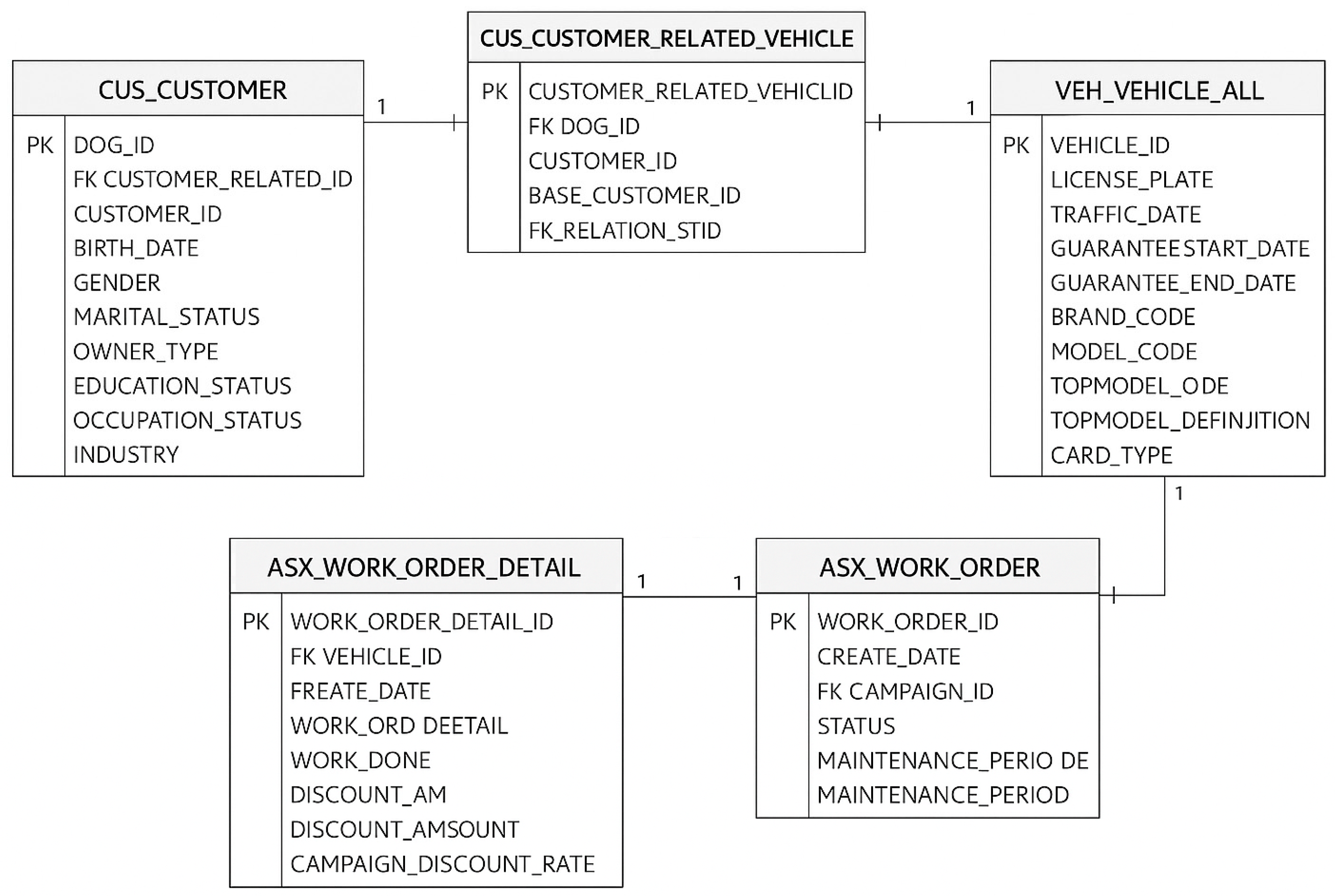
To ensure the dataset reflects realistic maintenance behavior, data related to previous vehicle owners was included in the training phase, while the test set was constructed solely based on the final owner of each vehicle to maintain behavioral consistency. All data extraction, transformation, and loading (ETL) procedures were automated using in-house Python (3.11 version) pipelines. The raw data was extracted from Oracle Database tables using DBeaver, an internal data access and visualization platform. Three primary tables—customer, vehicle, and maintenance—served as the foundational data sources. These tables were linked using T-SQL queries, with foreign key (FK) and primary key (PK) constraints to establish relational integrity. The entity relationship and the joining mechanism between these tables are visualized in Figure 1.

The preprocessing logic, including filtering and joining, was partially implemented in SQL and partially in Python, following a modular pipeline architecture. In the SQL layer, data joining operations between customer, vehicle, and maintenance tables were executed using T-SQL. Additionally, domain-specific filtering rules—such as restricting the data to certain vehicle brands, filtering records within a defined service date range, and excluding invalid entries—were applied directly within the database environment for efficiency and scalability.

In the Python layer, advanced data preprocessing tasks were programmatically applied to the extracted datasets, including

○

Imputation of missing values (using median for numerical and mode for categorical features);

○

Outlier detection and treatment (via Z-score and domain-specific thresholds);

○

Feature scaling, including both standardization and normalization where appropriate;

○

Encoding of categorical variables through one-hot encoding and frequency encoding;

○

Creation of derived and interaction-based features to enhance model interpretability;

○

Application of class imbalance strategies, such as class_weight = ‘balanced’.

This hybrid preprocessing strategy ensured the balance between efficiency (SQL operations close to source) and flexibility (Python for modeling-specific transformations). It also improved reproducibility and modularity across iterative model development phases. A comprehensive description of all 60 attributes, their sources, and transformations is available in

Table A1. Attributes, data sources, inferred type, and meanings.

No	Attribute	Data Source	Inferred Type	Usage
1	Customer ID	Customer Data	Identifier/Date	It specifies the vehicle owner’s ID.
2	Chassis ID	Vehicle Data	Identifier/Date	It indicates the chassis number of the vehicle.
3	Vehicle ID	Vehicle Data	Identifier/Date	It indicates the vehicle number of the vehicle.
4	Work Order ID	Maintenance Data	Identifier/Date	It specifies a work order number for each maintenance record.
5	Count of Owner	Derived Data	Numerical	It indicates the total number of customers who have owned the vehicle.
6	Service Visit Date	Maintenance Data	Identifier/Date	It represents the maintenance service date represented in this line.
7	Previous Service Visit Date	Derived Data	Identifier/Date	It represents the vehicle’s previous Service Visit Date.
8	Days Between Service Visits	Derived Data	Numerical	It represents the number of days between the previous maintenance service visit and this maintenance service visit.
9	Number of Service Visits—Car and User	Derived Data	Numerical	It represents the number of days between the previous maintenance service visit and this maintenance service visit.
10	Previous Total Net Amount	Derived Data	Numerical	It represents the fee paid for previous maintenance services.
11	Previous Total Discount Amount	Derived Data	Numerical	It indicates the discount amount applied to previous maintenance services.
12	Previous Total Campaign Discount Amount	Derived Data	Numerical	It represents the amount of TL-based discount applied through the campaign in the previous maintenance service.
13	Car Age—Day	Derived Data	Numerical	It represents the vehicle age in days.
14	Car Age—Month	Derived Data	Numerical	It indicates the vehicle age in months.
15	Car Age	Derived Data	Numerical	It represents the vehicle age in years.
16	Guarantee Remaining Day	Derived Data	Numerical	It indicates the number of days remaining from the vehicle’s warranty period.
17	Guarantee End Date	Vehicle Data	Identifier/Date	It represents the end date of the vehicle’s warranty period.
18	Visited	Derived Data	Target Variable	It represents whether the vehicle has come to the maintenance service. For each customer vehicle, we look at whether it comes for each month in a certain period. If it came in January, this line would appear as 1. If it has not arrived in other months, the visited field will appear 0.
19	Number of Service Visits—User	Derived Data	Numerical	It represents the total number of times the relevant customer brought their vehicle to the service for maintenance purposes.
20	Number of Service Visits—Car	Derived Data	Numerical	It represents the total number of times the relevant vehicle has been to the service for maintenance purposes.
21	Previous Total Discount Amount– Euro	Derived Data	Numerical	It represents the amount of discount in euros applied in the previous maintenance service.
22	Previous Total Campaign Discount Amount—Euro	Derived Data	Numerical	It represents the amount of discount in euros applied through the campaign in the previous maintenance service.
23	Previous Total Net Amount—Euro	Derived Data	Numerical	It represents the fee paid for previous maintenance services in euro terms for the relevant day.
24	Number of Active Car	Derived Data	Numerical	It represents the fee paid for previous maintenance services in euro terms for the relevant day.
25	Days Since Last Car	Derived Data	Numerical	It represents the number of days since the customer’s last vehicle purchase.
26	Maximum Total Net Amount—Euro	Derived Data	Numerical	It represents the highest amount paid by the customer for maintenance services in euros.
27	Cumulative Total Net Amount—Euro	Derived Data	Numerical	It represents the total amount paid by the customer for all maintenance services in euros.
28	Lagged Days Between Service Visits	Derived Data	Numerical	It refers to the number of days since the previous maintenance service that the customer went with the relevant vehicle.
29	Cumulative Days Between Service Visits	Derived Data	Numerical	It refers to the cumulative total of the number of days passed between the customer’s vehicle and the maintenance services the customer went to.
30	Average Days Between Service Visits	Derived Data	Numerical	It represents the average number of days between the customer’s date to bring the relevant vehicle to maintenance service.
31	Standard Deviation of Days Between Service Visits	Derived Data	Numerical	It represents the standard deviation of the number of days between the customer’s time to bring the relevant vehicle to maintenance service.
32	Months Between Service Visits	Derived Data	Numerical	It represents the number of months between the vehicle’s previous service visit and this service visit.
33	Years Between Service Visits	Derived Data	Numerical	It represents the number of years between the vehicle’s previous service visit and this service visit.
34	Previous Total Campaign Discount Rate	Derived Data	Numerical	It represents the percentage change between the discount applied through the campaign in the previous maintenance service visit and the discount applied in this maintenance service visit.
35	Previous Total Discount Rate	Derived Data	Numerical	It represents the percentage change between the discount applied for the previous maintenance service visit and the discount applied for this maintenance service visit.
36	Lagged Percent Difference on Service Fee	Derived Data	Numerical	It represents the percentage change between the price paid at the previous maintenance service visit and the price paid for this maintenance service visit.
37	Lagged Mileage from Last Service Visit	Derived Data	Numerical	It represents the mileage difference between the vehicle’s previous maintenance service and this maintenance service.
38	Plate Province	Vehicle Data	Categorical	It represents the province to which the vehicle’s license plate is connected.
39	Brand Code	Vehicle Data	Categorical	It represents the brand of the vehicle.
40	Top Model Code	Vehicle Data	Categorical	It represents the top model of the vehicle.
41	Top Model Definition	Vehicle Data	Categorical	It represents the detailed top model description of the vehicle.
42	Base Model Code	Vehicle Data	Categorical	It represents the base model of the vehicle.
43	Customer Type	Customer Data	Categorical	It represents the type of customer.
44	Gender	Customer Data	Categorical	It represents the gender of the customer.
45	Birth Year	Customer Data	Numerical	It represents the customer’s year of birth.
46	Marital Status	Customer Data	Categorical	It represents the marital status of the customer.
47	Education Status	Customer Data	Categorical	It represents the customer’s educational status.
48	Occupation	Customer Data	Numerical	It represents the client’s profession.
49	Industry	Customer Data	Categorical	It represents the industry in which the customer works.
50	Nationality	Customer Data	Categorical	It represents the nationality of the client.
51	Mileage per Day	Derived Data	Numerical	It represents the average kilometer traveled by the customer with the relevant vehicle in a day.
52	Service Visit per Year	Derived Data	Numerical	It represents the average number of times the vehicle comes to maintenance service yearly.
53	User & Car Z-score	Derived Data	Numerical	It expresses how much the date we predict for the customer deviates from that person’s habit.
54	DSG Ratio	Derived Data	Numerical	It represents the rate of encountering DSG gearbox-related problems in vehicles.
55	Benchmark Estimation	Derived Data	Numerical	The rule-based filtering method represents the estimation of whether the customer will come with the vehicle on the relevant date.
56	Churned Customer	Derived Data	Numerical	It indicates whether the customer has had her vehicle serviced for a long time.
57	Service Year	Derived Data	Numerical	It refers to the maintenance service year that the vehicle came in the corresponding record.
58	Service Month	Derived Data	Numerical	It refers to the maintenance Service Month in which the vehicle came in the relevant record.
59	Last Service Year	Derived Data	Numerical	It refers to the vehicle’s previous maintenance service year.
60	Last Service Month	Derived Data	Numerical	It refers to the vehicle’s previous maintenance Service Month.

of Appendix A. An illustration of the overall data acquisition and enrichment flow is provided in Figure 2.

3.3. Data Analysis

After the dataset was created, the relationships between different features in the dataset needed to be determined. The dataset was analyzed in two stages: descriptive statistics and exploratory data analysis.

3.3.1. Descriptive Statistics

The dataset used in this study was obtained from the CRM and after-sales service records of a leading automotive company, spanning a timeframe from January 2012 to December 2021. It contains monthly snapshots, representing customer–service interaction records over a span of 120 months. It consists of 108,596 visited service records, involving 3872 unique customers and 13,201 vehicles. While the company database contains a significantly larger volume of customer and vehicle records, this subset was selected as a pilot dataset to validate the modeling approach and conduct controlled experimentation. Importantly, the entire dataset was used in the exploratory data analysis (EDA) and feature engineering stages to capture overall behavioral patterns and ensure the robustness of derived features. However, only the pilot subset was utilized in the model training and testing phases to maintain consistency and interpretability, as well as to enable efficient experimentation under a controlled scope.

Although a single customer may own multiple vehicles and vehicle ownership can change over time, our modeling strategy is structured around the last known owner of each vehicle. This decision was made to avoid behavioral inconsistencies, as the maintenance patterns and service usage habits may differ significantly between previous and current owners. While historical records—including data from previous owners—are utilized during model training to enrich the feature space and learn general patterns, the test set is exclusively constructed using actions and interactions associated with the final owner of each vehicle. This approach ensures that model predictions are contextually relevant and aligned with the actual decision-making behavior of the most recent customer, which is critical for operational deployment.

The primary aim was to predict whether a customer would visit the service center in the subsequent month, modeled as a binary classification problem (VISITED = 1 or 0). As illustrated in Figure 3, the dataset exhibits a highly imbalanced distribution of the target variable VISITED, which indicates whether a customer has visited the service center in a given period.

○

Positive class (VISITED = 1): 108,596 records;

○

Negative class (VISITED = 0): 1,201,319 records;

○

Total records: 1,309,915.

The initial dataset consisted of 60 features, which are detailed in Table A1 in Appendix A along with their definitions and data sources.

Among the 60 features, 7 are identifier/date (see

Table 1. Type of identifier/date features.

Attribute	Data Source	Inferred Type
Customer ID	Customer Data	Identifier/Date
Chassis ID	Vehicle Data	Identifier/Date
Vehicle ID	Vehicle Data	Identifier/Date
Work Order ID	Maintenance Data	Identifier/Date
Service Visit Date	Maintenance Data	Identifier/Date
Previous Service Visit Date	Derived Data	Identifier/Date
Guarantee End Date	Vehicle Data	Identifier/Date

). During the preprocessing phase, identifiers (e.g., Customer ID, Chassis ID) and date-type variables (e.g., Service Visit Date, Guarantee End Date) were excluded from modeling, as they are not directly informative for prediction or are used for partitioning purposes.

Among the 60 features, 11 are categorical variables (see

Table 2. Types of categorical features.

Attribute	Data Source	Inferred Type
Plate Province	Vehicle Data	Categorical
Brand Code	Vehicle Data	Categorical
Top Model Code	Vehicle Data	Categorical
Top Model Definition	Vehicle Data	Categorical
Base Model Code	Vehicle Data	Categorical
Customer Type	Customer Data	Categorical
Gender	Customer Data	Categorical
Marital Status	Customer Data	Categorical
Education Status	Customer Data	Categorical
Industry	Customer Data	Categorical
Nationality	Customer Data	Categorical

). Categorical variables in the dataset (such as gender, Customer Type, Plate Province, Brand Code, etc.) were transformed into numerical representations to enable their use in machine learning models. The transformation is described in Section 4.1.5. Some categorical variables were eliminated on a model basis, as explained in Section 4.2.8, by evaluating the significance they added to the model.

Among the 60 features, 41 are numeric variables (see

Table 3. Types of numeric features.

Attribute	Data Source	Inferred Type
Count of Owner	Derived Data	Numerical
Days Between Service Visits	Derived Data	Numerical
Number of Service Visits—Car and User	Derived Data	Numerical
Previous Total Net Amount	Derived Data	Numerical
Previous Total Discount Amount	Derived Data	Numerical
Previous Total Campaign Discount Amount	Derived Data	Numerical
Car Age—Day	Derived Data	Numerical
Car Age—Month	Derived Data	Numerical
Car Age	Derived Data	Numerical
Guarantee Remaining Day	Derived Data	Numerical
Number of Service Visits—User	Derived Data	Numerical
Number of Service Visits—Car	Derived Data	Numerical
Previous Total Discount Amount– Euro	Derived Data	Numerical
Previous Total Campaign Discount Amount—Euro	Derived Data	Numerical
Previous Total Net Amount—Euro	Derived Data	Numerical
Number of Active Car	Derived Data	Numerical
Days Since Last Car	Derived Data	Numerical
Maximum Total Net Amount—Euro	Derived Data	Numerical
Cumulative Total Net Amount—Euro	Derived Data	Numerical
Lagged Days Between Service Visits	Derived Data	Numerical
Cumulative Days Between Service Visits	Derived Data	Numerical
Average Days Between Service Visits	Derived Data	Numerical
Standard Deviation of Days Between Service Visits	Derived Data	Numerical
Months Between Service Visits	Derived Data	Numerical
Years Between Service Visits	Derived Data	Numerical
Previous Total Campaign Discount Rate	Derived Data	Numerical
Previous Total Discount Rate	Derived Data	Numerical
Lagged Percent Difference on Service Fee	Derived Data	Numerical
Lagged Mileage from Last Service Visit	Derived Data	Numerical
Birth Year	Customer Data	Numerical
Occupation	Customer Data	Numerical
Mileage per Day	Derived Data	Numerical
Service Visit per Year	Derived Data	Numerical
User and Car Z-score	Derived Data	Numerical
DSG Ratio	Derived Data	Numerical
Benchmark Estimation	Derived Data	Numerical
Churned Customer	Derived Data	Numerical
Service Year	Derived Data	Numerical
Service Month	Derived Data	Numerical
Last Service Year	Derived Data	Numerical
Last Service Month	Derived Data	Numerical

). A feature selection process was applied on a per-model basis among some numerical features. This process eliminated five features that showed low importance scores or poor correlation with the target variable across models. The steps performed in feature selection are explained in detail in Section 4.2.8.

Among the 60 features, 1 is the target variable.

Table 4. Type of numeric features.

Attribute	Data Source	Inferred Type
Visited	Derived Data	Target Variable

presents the type of annotation of numeric features used in the modeling process. Among these, VISITED is identified as the target variable, representing whether a customer visited the service center in a given month. This binary feature (1 = visited, 0 = not visited) forms the foundation of the classification task addressed in this study.

These features include both raw attributes directly extracted from operational databases (e.g., Customer ID, Chassis ID, Vehicle ID, Work Order ID, Service Visit Date, Maintenance Period) and engineered variables specifically created to improve model interpretability and predictive power. An example of an engineered feature is Days Between Service Visits, which quantifies the number of days between the current and previous maintenance visits, providing temporal insight into service behavior.

The final training dataset thus consisted of 48 refined features used for model development. This hybrid approach, combining domain-derived raw variables and carefully crafted engineered features, aimed to enhance both the semantic meaning and predictive capability of the input data. A statistical summary of some selected attributes for visited and non-visited records is presented in

Table 5. Statistical summary of visited records.

	Visited Records			Non-Visited Records
Attribute	Mean	Standard Deviation	Median	Mean	Standard Deviation	Median	p-Value
Maintenance Period (year)	11.32	8.62	16.00	10.71	8.60	16.00	0.00
Days Between Service Visits	353.23	195.08	350	370.87	234.97	336	0.00
Car Age (Years)	2.86	2.11	2.19	2.95	2.23	2.38	0.00
Remaining Guarantee Days	129.87	181.80	0.00	137.23	201.30	0.00	0.00
Previous Total Net Amount (EUR)	245.75	120.32	230	0.00	0.00	0.00	0.00
Previous Total Discount Amount (EUR)	20.15	15.22	15.00	0.00	0.00	0.00	0.00
Mileage per Day (km)	55.80	23.50	50.00	58.75	25.60	55.00	0.02
Number of Service Visits (User)	3.25	1.20	3.00	1.00	0.00	1.00	0.00
Cumulative Days Between Service Visits	1	0	1	0	0	0	-
Guarantee End Date (Year)	2024.50	0.75	2024	2025.20	0.85	2025	0.01
DSG Ratio	0.12	0.05	0.10	0.08	0.03	0.07	0.00
Cumulative Total Net Amount (EUR)	800.75	350.20	750.00	0.00	0.00	0.00	0.00

.

The Maintenance Period attribute reflects the time (in years) from the vehicle’s purchase date to its maintenance service date. For example, if a vehicle is serviced for the first time in January 2021, the Maintenance Period is recorded as 1 for that service visit. However, if the vehicle does not visit the service center for the remaining 11 months of the year, a Maintenance Period of 0 is assigned for the months when no service occurs. Non-visited records are derived as dummy records from the visited ones and thus inherit the same Maintenance Period values. As demonstrated in Table 5, this leads to similar mean and standard deviation values for both visited and non-visited records.

The Days Between Service Visits attribute shows a higher mean for non-visited records compared to visited ones. This discrepancy occurs because non-visited records represent consecutive months where no maintenance service happens. Over time, the number of days since the last service increases for these vehicles, causing higher averages and more variability. In contrast, visited records reset the count after each service visit, resulting in a lower average for the time between visits. As shown in Table 5, non-visited records exhibit greater variability, reflected by a larger standard deviation compared to the visited records. The p-value (≤0.05) indicates that this difference is statistically significant, confirming that the time between service visits is significantly longer for non-visited vehicles.

The Car Age attribute is a decimal value that increases monthly for each vehicle, reflecting the vehicle’s age in years. With each new record, whether for a visited or non-visited vehicle, the Car Age slightly increases. While the mean and standard deviation values are close for both visited and non-visited records, the mean Car Age for non-visited records is slightly higher, which is largely due to their larger count. As shown in Table 5, this difference is statistically significant (p-value ≤ 0.05), indicating that non-visited records generally correspond to older vehicles compared to those that were regularly serviced.

The Remaining Guarantee Days is lower for visited records compared to non-visited ones due to several factors. Passenger vehicles typically undergo 1–2 maintenance visits per year. For instance, if a record shows X days left until the warranty expires, this value decreases by approximately 365 days with the next service visit. In contrast, non-visited records see a slower reduction in warranty days, as the count decreases incrementally month by month. Additionally, a significant portion of vehicles in the dataset are already out of warranty, which is why the median Remaining Guarantee Days for both groups is 0, as shown in Table 5. The statistically significant p-value (≤0.05) confirms a meaningful difference between the two groups in terms of remaining warranty days.

The Visits feature is binary, representing whether a vehicle visited the service center (1) or not (0) during a given month. As shown in Table 5, the mean value for visited records is 1.00, as all visited records inherently reflect a service visit. Similarly, the standard deviation and median for visited records are 0.00 and 1.00, respectively, confirming that all visited entries in the dataset are consistent with the definition of this feature. Conversely, for non-visited records, the mean and standard deviation are 0.00, as they exclusively represent months when no service occurred. This binary structure provides clear separation between the two groups and does not require a statistical p-value comparison. Instead, the feature effectively differentiates the dataset into two distinct segments for further analysis. Discount amounts are naturally higher for visited records since discounts are only applied when a vehicle is serviced. Non-visited records have a consistent value of EUR 0, as no service occurred to warrant a discount. The data confirms this expected difference, and the p-value (≤0.05) indicates that the disparity in mean discount amounts is statistically significant.

Interestingly, non-visited records show a slightly higher mean for Mileage per Day (km). This could be attributed to vehicles that continue to accumulate mileage without visiting a service center. In contrast, visited records often reflect intervals when vehicles underwent maintenance, which may reduce the average daily usage temporarily. The p-value (≤0.05) further validates that this difference is meaningful.

Unsurprisingly, the mean Number of Service Visits (User) is much higher for visited records since these inherently represent actual maintenance events. On the other hand, non-visited records capture months with no service visits, which naturally lowers their mean value. The statistically significant p-value (≤0.05) confirms this difference, aligning with the expected behavior of the dataset.

For non-visited records, the Cumulative Days Between Service Visits is notably higher. This occurs because non-visited records continue to accumulate time gaps between maintenance events. Visited records, however, reset this duration after each service visit, leading to a comparatively lower cumulative value. The statistically significant p-value (≤0.05) reinforces the significance of this observation.

The mean Guarantee End Date (Year) tends to be slightly higher for non-visited records. This might be because non-visited records often represent vehicles earlier in their warranty period, while visited records include more vehicles nearing the end of their warranty coverage. The p-value (≤0.05) confirms that this difference is statistically significant, reflecting trends in vehicle warranty expiration across the dataset.

The DSG Ratio is notably higher for visited records, likely because vehicles experiencing DSG gearbox-related issues are more frequently brought in for maintenance. Non-visited records, in contrast, may correspond to vehicles without such problems or to owners who opt for independent repairs. The statistically significant p-value (≤0.05) highlights the importance of this finding.

As expected, visited records show a significantly higher mean for Service Visits per Year. This is because these records reflect actual maintenance activity, whereas non-visited records represent months without service events. The p-value (≤0.05) confirms the statistical significance of this difference, underscoring the behavioral contrast between the two groups.

3.3.2. Exploratory Data Analysis

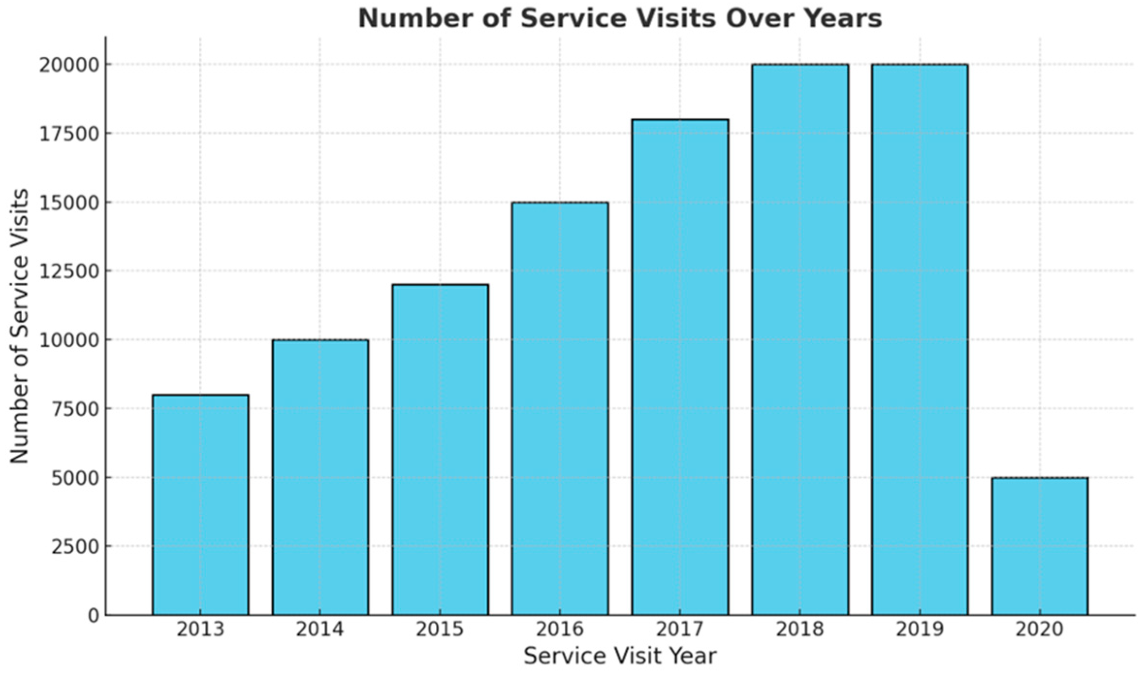
This section examines the features in the dataset and the dependent changes of these features. Figure 4 visualizes the total number of maintenance service records by year. While the number of services increased gradually until 2019, the number of visits started to decrease in 2019 and beyond. The COVID-19 pandemic, which started in 2019, had an impact on this decrease. Vehicle owners who do not leave their homes and do not use their vehicles may not need to have their vehicles serviced.

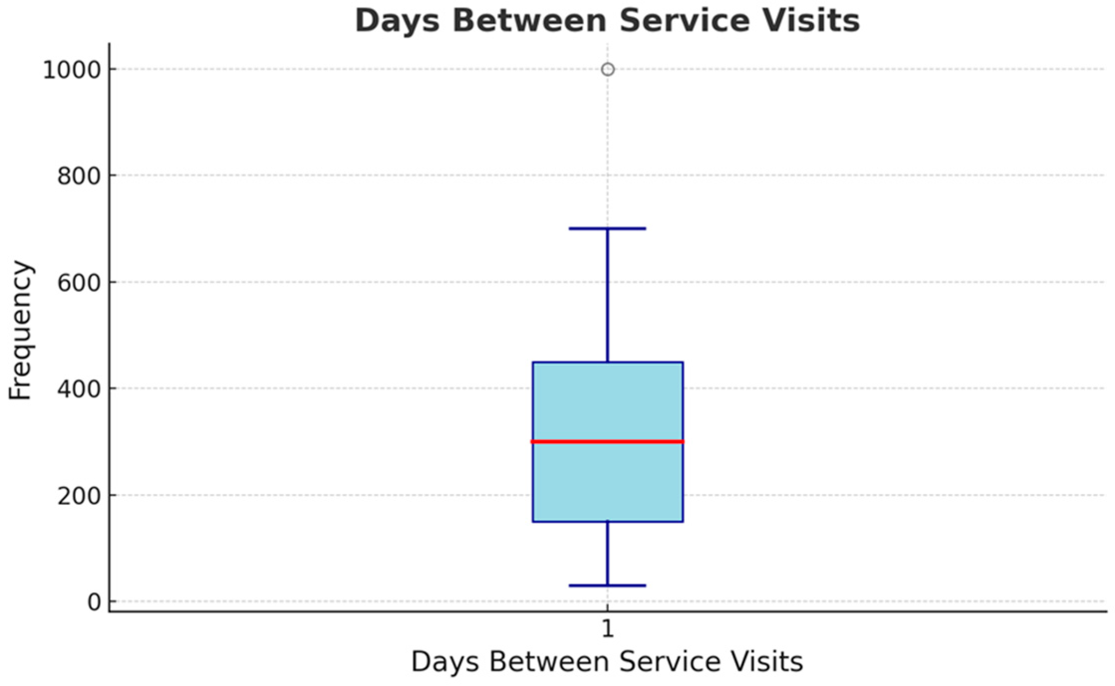
Figure 5 examines the time between the vehicles visiting for maintenance. The median value is 382 days, and customers’ visit habits vary considerably. In addition, different Maintenance Periods can be assumed for other vehicles. Hence, the time between two treatments can vary greatly depending on the car brand or type.

To elaborate on the variability mentioned in Figure 5, we present a comparison of Days Between Service Visits for two anonymized brands (Brand A and Brand B). As shown in Figure 6, Brand A vehicles exhibit a shorter median service interval (~210 days), while Brand B vehicles tend to have longer intervals (~380 days) between maintenance visits. This variation may be attributed to differences in usage patterns. Brand A is commonly used for commercial or fleet operations, leading to higher mileage and more frequent maintenance needs. In contrast, Brand B includes more private or premium-use vehicles, which are serviced less frequently. This insight supports our assertion regarding the effect of vehicle type and usage context on service behavior.

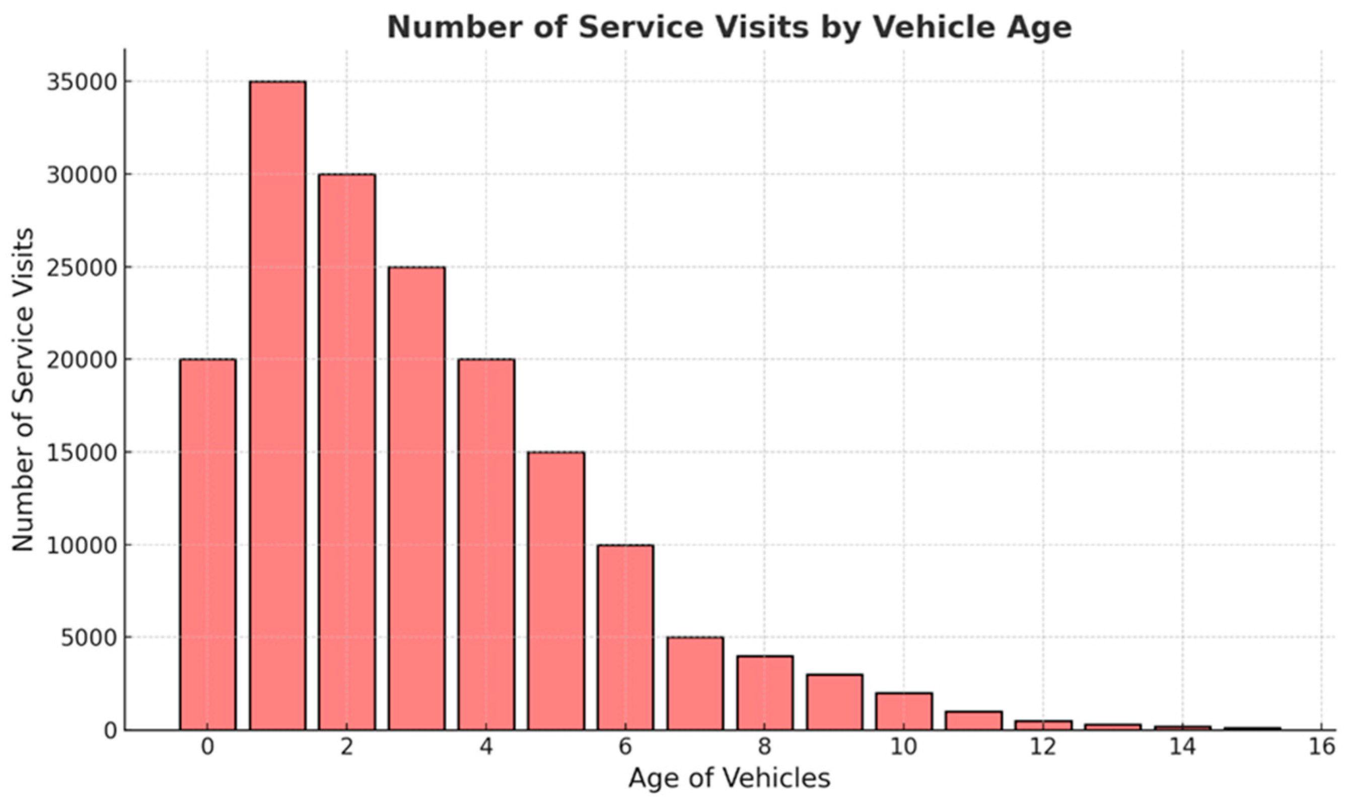
Figure 7 analyzes the number of maintenance visits according to vehicle age. It has been observed that the number of maintenance visits decreases as the age of the vehicle increases. There are two main reasons for the decline here: the 2-year warranty period and the economic advantage of special services. The decrease in the number of services starts from the age of 2 years. Vehicles are under warranty for two years from the date of purchase. Owners continue to take their vehicles to authorized service centers so that the vehicle’s warranty is not impaired. After the vehicle turns two years old, the habit of bringing it to authorized services may decrease. Another reason for this decline is the customers’ deviation from authorized service providers to secondary, non-authorized repair stations due to their lower maintenance service prices.

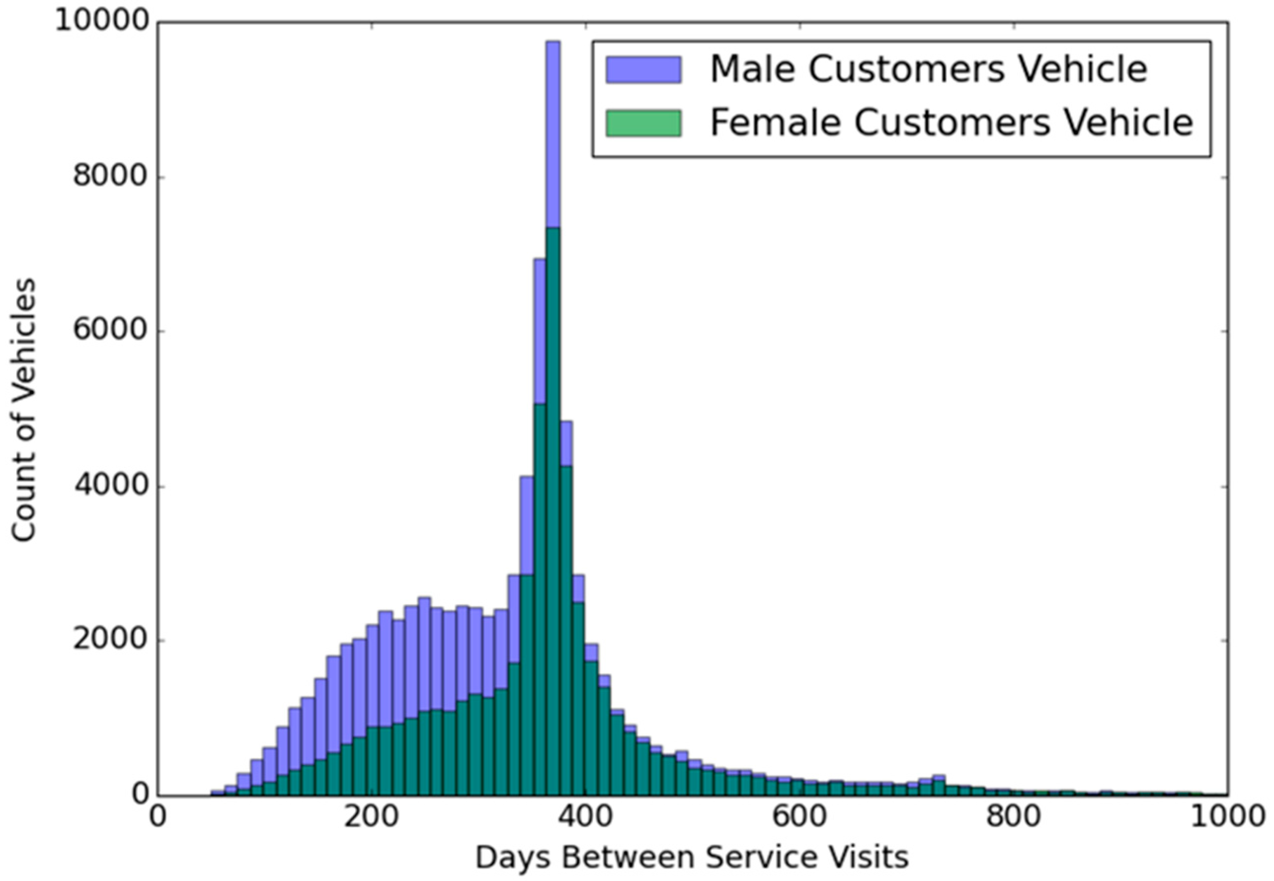
The distribution of time between maintenance visits of male and female customer vehicles is visualized in Figure 8. According to this visual analysis, after the number of days between two maintenance exceeds 400, regardless of gender, the number of maintenance service records decreases.

In addition to the visual analysis in Figure 8, we calculated descriptive statistics for the Days Between Service Visits across genders. For male customers, the average interval was approximately 340 days with a standard deviation of 185 days, while female customers exhibited a slightly higher average of 370 days, with a standard deviation of 205 days. These values align with the visual trends, where male customer vehicles display a sharper peak around the 300–350 day range, suggesting more frequent and routine maintenance behavior. In contrast, female customer vehicles demonstrate a broader spread, indicating a tendency toward longer intervals between service visits. The overall dataset shows a mean of 353.2 days, median of 350 days, and standard deviation of 195.1 days, confirming that most vehicles are serviced annually, with some variability across customer segments.

In Figure 9, the distribution of the measured kilometers of the vehicles during the service visits is examined. We observe that measurements are made at approximately 15,000 km for most vehicles. The reasons for the density at 15,000 km are that the vehicle is usually less than two years old and under warranty.

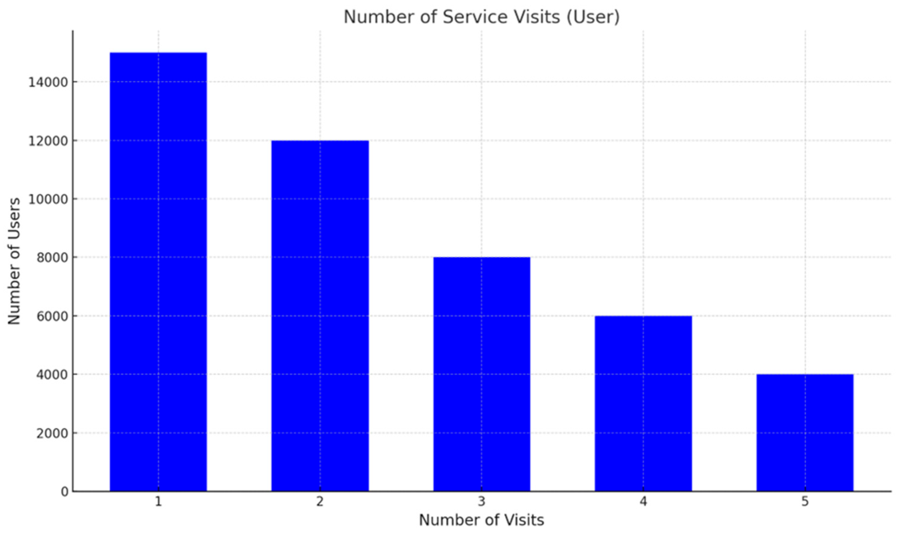
Figure 10 illustrates the distribution of users based on the number of service visits made to authorized centers. The data reveals a clear decreasing trend, where the number of users declines as the number of service visits increases. Specifically, the highest user concentration is observed among those who have visited authorized service centers only once, totaling approximately 15,000 users. This figure gradually decreases with each additional visit, with around 12,000 users for two visits, 8000 users for three visits, 6000 users for four visits, and 4000 users for five visits.

This pattern indicates that a significant proportion of customers engage with authorized service centers only for initial or occasional visits, while fewer customers exhibit frequent engagement. Such behavior could be attributed to factors such as cost sensitivity, alternative service options, or a lack of perceived value in returning to authorized centers after the initial visits.

From an operational perspective, this insight underscores the need for strategies that encourage repeat visits, particularly among customers who tend to stop after the first or second engagement. Personalized marketing campaigns, loyalty programs, or tailored incentives may serve as effective tools to retain these users and enhance their lifetime value. Furthermore, identifying the underlying reasons for the drop-off after one or two visits could provide actionable insights to address customer concerns and improve retention rates.

This declining pattern highlights the importance of customer retention strategies in ensuring the sustainability of authorized service centers, particularly in competitive markets where alternatives such as unauthorized service providers are readily available.

4. Methodology

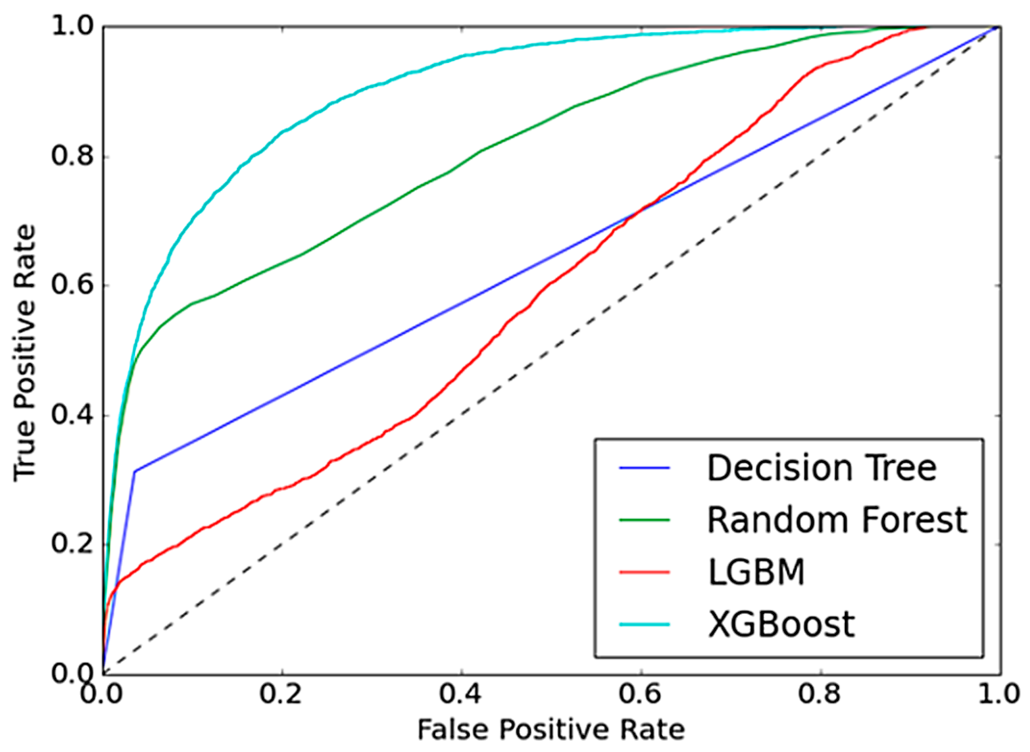
To develop a probabilistic prediction model for forecasting both workforce transitions and customers’ choices of authorized maintenance services, four supervised machine learning algorithms were employed: Decision Tree (DT), Random Forest (RF), Light Gradient Boosting Machine (LightGBM), and Extreme Gradient Boosting (XGBoost). The predictive performance of each model was compared using a resampling-based evaluation method, specifically k-fold cross-validation, to ensure robustness and mitigate overfitting. The proposed methodology consists of four major phases which are data collection, data preprocessing, model training and feature selection.

4.1. Data Preprocessing

In this phase, the raw data underwent a series of transformation steps.

4.1.1. Imputation of Missing Values

To ensure the quality and integrity of the dataset, missing values were thoroughly analyzed and imputed using appropriate statistical techniques depending on the nature and distribution of each feature. To ensure the quality and integrity of the dataset, missing values were thoroughly analyzed and imputed using appropriate statistical techniques depending on the nature and distribution of each feature. For instance, the variable Mileage per Day, which reflects the average distance driven by a customer per day, exhibited missing values, primarily due to inconsistencies in odometer data entries during service visits. Since the distribution of this feature was slightly right-skewed and contained some extreme values, median imputation was applied to preserve the central tendency while reducing the influence of outliers.

Similarly, for categorical features such as marital status and Education Status, missing values were imputed using the mode (i.e., most frequent category), assuming that missingness in such cases was random and not systematically biased. In contrast, variables with a high rate of missing values due to human input errors (e.g., Previous Service Fault Code and Previous Service Fault Description, where the missingness reaches almost 50%) were excluded from prediction-based strategies. These variables were not incorporated into modeling due to concerns over data quality and reliability and were instead handled separately or omitted altogether, depending on their relevance to the prediction task.

These imputation strategies were selected to balance the trade-off between data completeness and preservation of variable distributions, ensuring reliable and unbiased input for subsequent modeling phases. The left plot of Figure 11 shows the raw distribution of the Mileage per Day feature, with a mean of 55.8 km and a median of 50.0 km, reflecting a moderately right-skewed structure. The right plot displays the post-imputation distribution using median filling, preserving the central tendency and mitigating the impact of outliers.

4.1.2. Detection and Treatment of Outliers

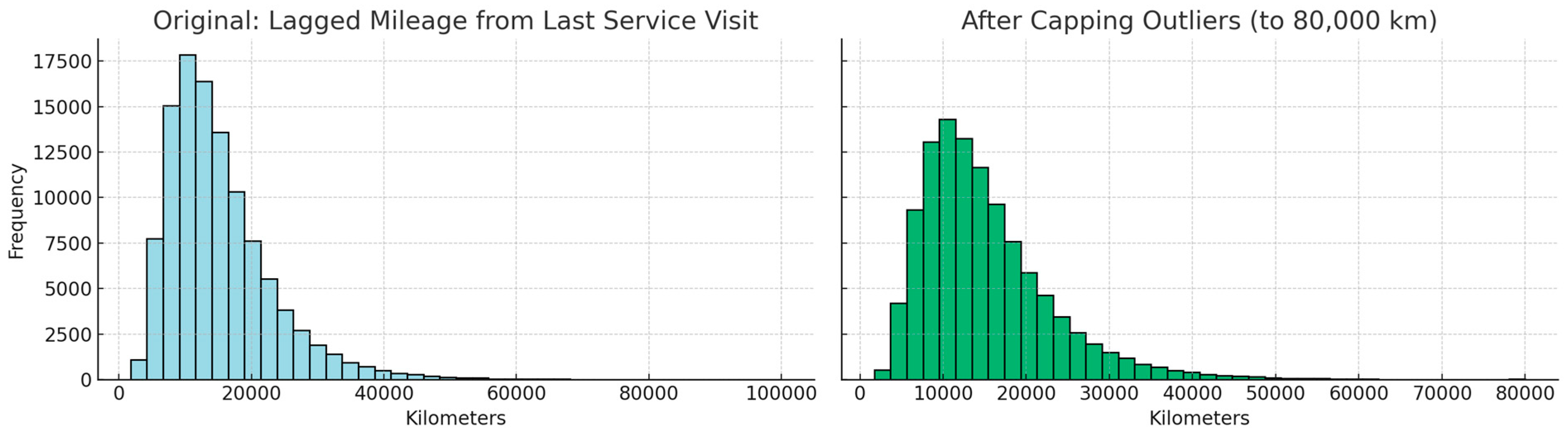
Outlier detection and treatment were carried out after imputing missing values and prior to feature scaling to ensure the integrity of feature distributions. Since extreme values may disproportionately influence threshold-based models and skew overall feature behavior, the interquartile range (IQR) method was applied for detecting outliers. Observations beyond the range of Q1 − 1.5 × IQR and Q3 + 1.5 × IQR were considered outliers and handled accordingly.

As a representative example, the feature Lagged Mileage from Last Service Visit exhibited a right-skewed distribution with a minority of records exceeding 60,000 km between visits. These high values likely resulted from data entry inconsistencies or rare usage patterns and were not reflective of general service behavior. Rather than removing such entries—which could risk loss of informative variance—a capping strategy was applied, restricting values above the IQR-based upper bound. This approach effectively reduced variance without compromising interpretability. Figure 12 illustrates the effect of this treatment, with a more condensed and statistically robust distribution observed after capping.

4.1.3. Feature Scaling (Standardization and Normalization as Appropriate)

Scaling is particularly crucial for algorithms that rely on distance metrics (e.g., k-NN, SVM) or gradient-based optimization (e.g., logistic regression, neural networks). In contrast, tree-based ensemble models such as Decision Tree (DT), Random Forest (RF), Light Gradient Boosting Machine (LightGBM), and Extreme Gradient Boosting (XGBoost) are inherently invariant to feature scaling, as they rely on threshold-based splitting rather than distance or magnitude comparisons.

Although the primary models employed in this study—Decision Tree (DT), Random Forest (RF), LightGBM, and XGBoost—are tree-based and theoretically invariant to feature scaling due to their reliance on threshold-based splitting, feature scaling was still applied for the following practical and methodological reasons:

○

Cross-Model Compatibility and Reusability

During exploratory phases and benchmarking, scaling-sensitive models such as logistic regression and Support Vector Machines were also considered. Applying consistent preprocessing ensures compatibility across different modeling scenarios without requiring duplicate pipelines.

○

Visualization and Interpretability

Scaled features provide better interpretability and comparability when visualizing feature distributions, detecting anomalies, or interpreting statistical patterns.

○

Future-Proofing and Pipeline Generalization

A standardized feature space is essential when developing reusable pipelines, deploying models in production, or integrating with hybrid systems (e.g., deep learning layers or clustering modules) that may require scaled inputs.

○

Model Ensemble Readiness:

Even when ensemble methods are composed of tree-based learners, they can be integrated into meta-modeling (stacking, blending) setups that include scale-sensitive components. Feature scaling supports seamless integration in such architectures. Depending on the distributional characteristics and modeling requirements of each feature, two primary scaling strategies were used:

• Z-score standardization (also known as standard scaling) was applied to variables that were approximately normally distributed or had symmetrical behavior. This transformation centers the data around zero with a standard deviation of one.
• Min–Max normalization was preferred for features that required bounded scaling in the [0,1] range, especially when used in models sensitive to absolute input magnitudes.

The choice between these two methods was based on each variable’s distribution, statistical properties (mean, median, standard deviation), and the expected influence on model convergence and performance.

One illustrative example of this process involves the Car Age (Years) feature. The left plot of Figure 13 shows its original distribution, with a mean of 2.86, standard deviation of 2.11, and median of 2.19, indicating a slightly right-skewed pattern.

In the middle plot of Figure 13, Z-score standardization is applied, transforming the values to have zero mean and unit variance. Although the core models used in this study—such as XGBoost, LightGBM, Random Forest, and Decision Tree—do not require feature scaling due to their split-based architecture, scaling was nonetheless explored to enhance model interpretability, facilitate potential downstream tasks, and prepare the data for possible hybrid model pipelines involving scaling-sensitive components.

The right plot of Figure 13 demonstrates Min–Max normalization, which bounds the values within the [0,1] range. While not essential for tree-based models, normalization can be particularly beneficial when integrating these features into dashboards, distance-based visualizations, or ensemble models with scale-sensitive learners.

The DSG Ratio represents the frequency of DSG gearbox-related issues and is inherently bounded between 0 and 1 with low variance (mean ≈ 0.12, std ≈ 0.05).

In the left panel of Figure 14, the original distribution shows a concentrated range around the mean. The middle plot of Figure 14 applies Z-score standardization, stretching the distribution to have unit variance. While this transformation is mathematically valid, it may over-amplify noise for low-variance features.

The right panel of Figure 14 uses Min–Max normalization, which preserves the bounded nature of the feature and is generally more appropriate for ratio-based or percentage-type variables. This approach ensures interpretability and compatibility, especially when features are combined or visualized.

The variable Number of Service Visits (User) represents the total number of services visits a customer has made with their vehicle. As a discrete variable with low cardinality (values range from 1 to 12), its original distribution of Figure 15 (left panel) is inherently grouped and resembles a categorical pattern.

The middle plot of Figure 15 applies Z-score standardization, which mathematically centers the values but has limited interpretive benefit due to the ordinal and low-range nature of the feature.

In the right panel of Figure 15, Min–Max normalization maps the values to the [0,1] range while preserving the ordinal structure. Although scaling is not strictly necessary for tree-based models like XGBoost or Random Forest, normalization may aid interpretability and visualization in exploratory data analysis or when integrating with other scaled features.

4.1.4. Creation of Derived or Interaction-Based Features to Enhance Predictive Power

To enrich the feature space and improve the model’s ability to capture complex patterns, a variety of derived and interaction-based features were engineered in addition to the raw attributes. This transformation aimed to encode domain-specific knowledge into structured numerical indicators, thus enhancing the predictive power of the learning algorithms.

For instance, Car Age (Years) was computed from service and registration dates to represent vehicle tenure. Mileage per Day was calculated by dividing cumulative mileage by vehicle age in days, standardizing customer usage patterns. Similarly, Service Visits per Year normalized service behavior over time, and Z-score (User and Car) quantified temporal deviation from a user’s typical service rhythm, highlighting anomalous visit timings. The DSG Ratio, on the other hand, reflected the historical failure rate of DSG gearboxes within similar model clusters, thereby embedding contextual mechanical risk.

These features were carefully selected and constructed through iterative analysis and consultation with domain experts. Notably, Table A1 in Appendix A provides a comprehensive overview of all raw and derived variables along with their definitions and modeling rationale, ensuring transparency and interpretability of the engineered feature set.

Together, these enhancements allowed the model to access latent relationships not readily visible in the raw data, leading to measurable gains in performance and generalization.

4.1.5. Encoding of Categorical Variables

Categorical variables in the dataset (such as gender, Customer Type, Plate Province, Brand Code, etc.) were transformed into numerical representations to enable their use in machine learning models. This transformation was performed using Scikit-learn’s OneHotEncoder for nominal features and LabelEncoder for ordinal ones where applicable.

In one-hot encoding, a categorical feature with k distinct values is converted into k binary columns. Mathematically, for a categorical variable x ∈ {$c_1,c_2,\dots ,c_k$}, the transformation can be represented as

$$\mathrm{OneHot}\left(x_i\right)=\left[1\left(x_i=c_1\right),1\left(x_i=c_2\right),\dots ,1\left(x_i=c_k\right)\right]$$

(1)

where 1(⋅) is the indicator function.

4.1.6. Class Imbalance Strategy and Weight Adjustment

To ensure robust and generalizable performance across diverse customer-vehicle records, we implemented a multi-model framework based on tree-based ensemble algorithms, including Decision Tree (DT), Random Forest (RF), Light Gradient Boosting Machine (LightGBM), and Extreme Gradient Boosting (XGBoost). These models were selected not only for their strong predictive performance on structured tabular data, but also for their inherent capacity to handle non-Gaussian distributions, high-cardinality features, and missing values.

An additional reason for selecting these models was their compatibility with imbalanced classification problems, which is a prominent challenge in the current dataset. Both LightGBM and XGBoost provide native support for class weighting through the scale_pos_weight parameter, enabling the model to compensate for skewed class distributions directly during training. Unlike traditional classifiers that require explicit resampling or synthetic data generation, tree-based ensemble methods can internally adjust for label imbalance without compromising model integrity or interpretability.

This approach was preferred over under-sampling, which would reduce the overall data volume and potentially discard informative patterns from the majority class. Moreover, over-sampling was avoided to prevent overfitting and synthetic noise in a structured business dataset. Class weighting, on the other hand, allowed the model to remain fully exposed to the original data distribution while compensating for skewed label frequencies at the optimization level.

The selected weight coefficients were computed as

$$\mathrm{s}\mathrm{c}\mathrm{a}\mathrm{l}\mathrm{e}\_\mathrm{p}\mathrm{o}\mathrm{s}\_\mathrm{w}\mathrm{e}\mathrm{i}\mathrm{g}\mathrm{h}\mathrm{t}={\displaystyle \frac{N_{negative}}{N_{positive}}}$$

(2)

and these values were fine-tuned using cross-validation to prevent over-penalization. The resulting models exhibited significantly improved recall and F1-scores for the minority class, confirming the effectiveness of this strategy. Details of the final weight values and associated performance metrics are provided in “Experimental Works”.

4.2. Model Training

To ensure robust and generalizable performance across diverse customer-vehicle records, we implemented a multi-model framework based on tree-based ensemble algorithms, including Decision Tree (DT), Random Forest (RF), Light Gradient Boosting Machine (LightGBM), and Extreme Gradient Boosting (XGBoost). These models were selected not only for their predictive strength on structured tabular data, but also for their capacity to accommodate the specific statistical characteristics observed in the dataset. These algorithms were specifically selected for the following reasons.

• Suitability for High-Dimensional and Heterogeneous Data

The dataset contains a mix of continuous (e.g., Days Between Service Visits) and categorical variables (e.g., Service Month, Churned Customer). Tree-based models inherently handle heterogeneous feature types without the need for extensive preprocessing or normalization, unlike models based on distance metrics (e.g., k-NN, SVM with RBF kernel).

• Handling of Non-linear Interactions

These models are capable of capturing non-linear relationships through recursive binary splits. For example, Decision Trees optimize a cost function such as the Gini index or Entropy:

$$\mathrm{Gini}=1-\sum _{i=1}^C{p}_i^2 \mathrm{o}\mathrm{r} \mathrm{Entropy}=-\sum _{i=1}^C{p}_i\log \left(p_i\right)$$

(3)

where $p_i$ is the proportion of class $i$ in a node. These criteria help models identify complex interaction patterns in the data, which are likely present given the diverse nature of service history and user behavior.

• Robustness to Multicollinearity and Outliers

Random Forest and Gradient Boosting algorithms (LightGBM, XGBoost) reduce overfitting and variance by aggregating multiple base learners. LightGBM and XGBoost further improve generalization through regularization terms in their objective functions:

$$\mathrm{Obj}\left(\theta \right)=\mathcal{L}\left(\theta \right)+\mathsf{\Omega }\left(\theta \right), \mathsf{\Omega }\left(\theta \right)=\gamma T+{\displaystyle \frac{1}{2}}\lambda \sum _{j=1}^T{w}_j^2$$

(4)

where $T$ is the number of leaves, $w_j$ represents leaf weights, and λ and γ are regularization parameters.

• Performance on Imbalanced and Sparse Labels

Given the imbalance in part replacement labels (binary flags for each part changed during service), boosting algorithms like XGBoost and LightGBM are advantageous due to their ability to focus on harder-to-classify examples via gradient-based loss optimization:

$$\mathrm{l}\left(y_i,\widehat{y_i}\right)=-\left(y_i\log \left(\widehat{y_i}\right)+\left(1-y_i\right)\log \left(1-\widehat{y_i}\right)\right)$$

(5)

where $y_i$ ∈ {0,1} is the label, and $\widehat{y_i}$ is the predicted probability.

• Computational Efficiency and Scalability

LightGBM uses histogram-based learning and leaf-wise tree growth with depth constraints, which improves speed and memory efficiency—important for production deployment and rapid retraining scenarios.

A key rationale for favoring tree-based methods was the non-Gaussian and often skewed nature of several critical numerical features, such as Cumulative Total Net Amount (EUR) and Days Between Service Visits, which deviated significantly from normality (see Figure 16).

In contrast to algorithms relying on distance metrics or feature scaling, ensemble tree models are inherently robust to such irregularities due to their use of threshold-based, greedy splits. Additionally, these models handle both high-cardinality categorical variables and missing values natively, reducing the need for aggressive preprocessing.

Each of the four machine learning models was trained independently using historical data:

For workforce transition modeling, historical employee records were used to learn the likelihood of job role changes or reskilling needs.

For customer maintenance modeling, service visit histories were used to predict the probability of future visits to authorized maintenance centers.

4.2.1. Model-Specific Hyperparameter Optimization and Validation Strategy

To determine the optimal hyperparameters for each model, we utilized Bayesian Optimization with Gaussian Process priors, which enables efficient exploration of the parameter space by balancing exploitation and exploration through probabilistic modeling of the objective function. This method was chosen over exhaustive grid or random search approaches due to its superior sample efficiency and convergence properties.

The optimization objective was based on 10-fold stratified cross-validation, where the F1-score on the validation folds was used to guide the search process. Final model performance was evaluated on a held-out test set that remained untouched during training and hyperparameter tuning to ensure unbiased generalization assessment.

Model selection and hyperparameter tuning were guided not only by performance metrics (e.g., F1-score, AUC, precision and recall) on the validation set but also by computational efficiency and model interpretability, which were critical considerations in an applied business environment and improvement. As seen in

Table 6. Extended hyperparameter search space for model optimization.

Model	Hyperparameter	Search Space
DT	max_depth	[2, 4, 6, 8, 10, 12, 15, 20]
	min_samples_split	[2, 5, 10, 20, 50]
	min_samples_leaf	[1, 2, 5, 10, 20]
	criterion	[“gini”, “entropy”]
	class_weight	[None, “balanced”, class imbalance ratio]
RF	n_estimators	[100, 250, 500, 750, 1000, 1250]
	max_depth	[4, 6, 8, 10, 12, 16, 20, 25]
	max_features	[“sqrt”, “log2”, 0.3, 0.5, 0.7]
	min_samples_split	[2, 5, 10, 20]
	min_samples_leaf	[1, 2, 5, 10]
	bootstrap	[True, False]
	class_weight	[None, “balanced”, class imbalance ratio]
LightGBM	n_estimators	[100, 250, 500, 750, 1000, 1500]
	max_depth	[−1, 4, 6, 8, 10, 12, 16]
	learning_rate	[0.005, 0.01, 0.02, 0.05, 0.1]
	min_child_samples	[5, 10, 20, 30, 50]
	subsample	[0.5, 0.6, 0.7, 0.8, 0.9, 1.0]
	colsample_bytree	[0.5, 0.6, 0.7, 0.8, 0.9, 1.0]
	scale_pos_weight	class imbalance ratio
XGBoost	n_estimators	[100, 300, 500, 750, 1000, 1500]
	max_depth	[3, 4, 6, 8, 10, 12, 16]
	learning_rate (eta)	[0.005, 0.01, 0.02, 0.05, 0.1]
	min_child_weight	[1, 3, 5, 10]
	subsample	[0.5, 0.6, 0.7, 0.8, 0.9, 1.0]
	colsample_bytree	[0.5, 0.6, 0.7, 0.8, 0.9, 1.0]
	gamma	[0, 0.1, 0.5, 1.0]
	scale_pos_weight	class imbalance ratio

, a detailed list of the selected hyperparameters and their respective values is provided.

4.2.2. Probabilistic Inference and Label Assignment

During testing, the trained models generated probabilistic outputs P ∈ [0,1] for each instance. These probabilities were binarized using a threshold value τ, as defined by the following rule:

$$Label=\left\{\begin{array}{c}1, if P \ge \tau \\ 0, if P<\tau \end{array}\right.$$

(6)

For the maintenance prediction model, a label of 1 signifies that the customer is expected to visit the service center, and 0 denotes no visit. While a threshold of 0.50 was used as the default, the optimal value of τ was determined empirically based on performance metrics (e.g., maximizing the F1-score or minimizing false negatives), as discussed in Section 5.

During testing, the trained models produced probability estimates P ∈ [0,1], which were binarized using a classification threshold τ. Although the default threshold τ = 0.50 is commonly used, in this study, the threshold value was not selected arbitrarily. Instead, we systematically evaluated a range of candidate thresholds at 0.05 intervals from 0.10 to 0.90 (i.e., τ ∈ {0.10, 0.15, 0.20, …, 0.90}).

For each threshold, we computed performance metrics on the validation set, including AUC, F1-score, and the precision–recall trade-off. In addition, we assessed two domain-specific impact measures, the Missed Service Opportunity Rate (MSOR) and the Excess Capacity Allocation Rate (ECAR), which reflect the operational costs associated with false negatives and false positives, respectively.

The evaluation revealed that a threshold of τ = 0.30 achieved the best overall balance—it yielded the highest AUC while simultaneously minimizing MSOR and ECAR. This indicates that 0.30 is not merely a default setting but represents a data-driven, domain-informed decision that aligns both predictive accuracy and business efficiency. Experimental results are discussed in detail in Section 5, but you can examine the different performance metrics obtained with some different thresholds in

Table 7. Threshold-specific model performance metrics including business-aware evaluation indicators (MSOR and ECAR).

Threshold	Algorithms	F1-Score	Recall	Precision	MSOR	ECAR
0.3	DT	0.30	0.31	0.29	0.71	0.69
	RF	0.40	0.57	0.31	0.69	0.43
	XGBoost	0.45	0.51	0.39	0.61	0.49
	LGBM	0.10	0.93	0.05	0.95	0.07
0.4	DT	0.30	0.31	0.29	0.71	0.69
	RF	0.43	0.43	0.43	0.57	0.57
	XGBoost	0.44	0.42	0.46	0.54	0.58
	LGBM	0.10	0.91	0.05	0.95	0.09
0.5	DT	0.30	0.31	0.29	0.71	0.69
	RF	0.39	0.32	0.51	0.49	0.68
	XGBoost	0.41	0.34	0.53	0.47	0.66
	LGBM	0.10	0.89	0.05	0.95	0.11
0.6	DT	0.30	0.31	0.29	0.71	0.69
	RF	0.32	0.22	0.56	0.44	0.78
	XGBoost	0.33	0.23	0.59	0.41	0.77
	LGBM	0.10	0.87	0.05	0.95	0.13

.

4.2.3. Decision Tree

Decision Trees (DT) often mimic human-level thinking, so they are understandable and interpretable. The Decision Tree algorithm, a hierarchical model, used to solve regression and classification problems, belongs to the family of supervised learning algorithms. The purpose of using a Decision Tree is to create a training model that can be used to predict the class or value of the target variable by learning the simple decision rules extracted from the training data.

The predictions will start from the node’s root and then compare the values of the root attribute with the other attribute. Impurity measurement is used to determine which attribute will be the root node. A measure of impurity also measures the goodness of subsequent splits [33]. Entropy and the Gini index can be used to measure impurity. The threshold values $w_{m0}$ must also be known to split the root node into two separate internal nodes. In the case where N is the root nodes, suppose that $N_m$ is the number of training instances reaching in node m. Among the $N_m$ data points, there are $N_{m-1}$ possible $w_{m0}$. We do not need to test all points. The best $w_{m0}$ is always between adjacent points belonging to different classes [33]. The samples are assigned to binary classes with the following function:

$$f_{\left(x\right)}:x_j>w_{m0}.$$

(7)

$C_i$ is the i class that will be split after the root node. Given that a sample reaches m nodes, the estimate for the probability of class $C_i$ is [33]

$$P\left(C_i|x,m\right)\equiv p_m^i\equiv {\displaystyle \frac{N_m^i}{N_m}}.$$

(8)

The Gini index used in this paper to measure impurity is calculated as [33]

$$\mathsf{\Phi } (p, 1-p)=2 p(1-p).$$

(9)

The Gini index function to measure node impurity is calculated as [33]

$$I_m={\sum }_{i=1}^K{p}_m^i{log}_2{p}_m^i.$$

(10)

If $p_m^i$ is 0 or 1 for all i, node m is pure. If the split is pure, we do not need any more splits, and we can add a leaf node labeled with the class where $p_m^i$is 1 [33]. If node m is not pure, then the instances should be split to decrease impurity, and there are multiple possible attributes on which we can split. We look for the split that minimizes impurity after the split because we want to generate the smallest tree. If the impurity in the nodes is equal to 0 or converges to a specified limit, the labeled leaf is created, and tree splitting is stopped.

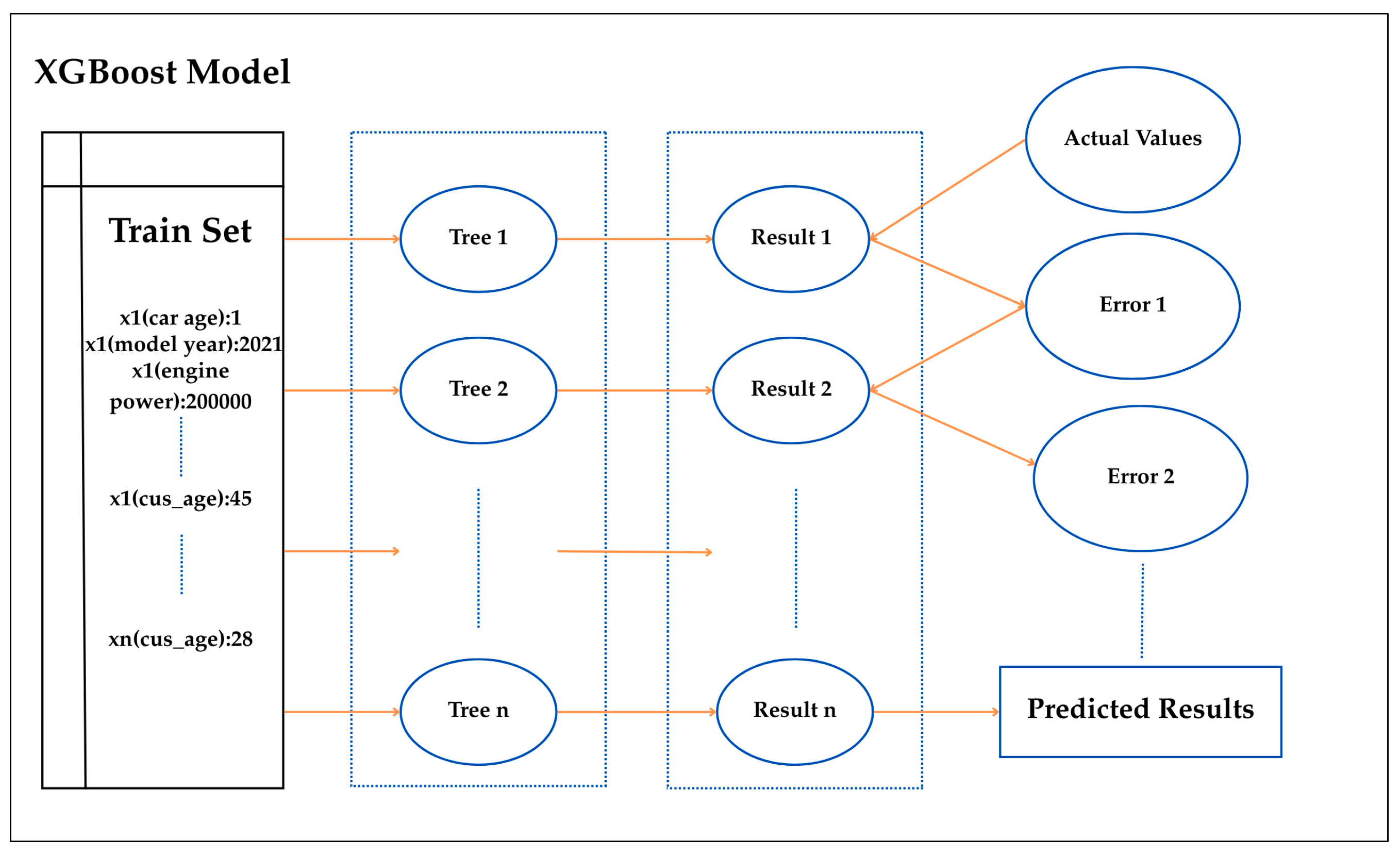
4.2.4. Extreme Gradient Boosting

Extreme Gradient Boosting (XGBoost) is a classification and regression algorithm based on the Gradient Boosting Decision Tree (GBDT), a supervised learning method based on function approximation by optimizing specific loss functions and applying several regularization techniques. [34] Figure 17 is the flowchart outlining the use of the XGBoost algorithm in this paper.

Suppose the training dataset D and the sample and target label in it are expressed as

$$D=\left\{\left(x_1,y_1\right),\left(x_2,y_2\right),\left(x_3,y_3\right),\left(x_4,y_4\right),\dots ,\left(x_n,y_n\right)\right\}$$

(11)

The prediction function of the $i^{th}$ sample is stated as [34]

$${\mathrm{ŷ}}_i=\sum _{n=1}^N{f}_n{(x}_n),f_n\in F$$

(12)

where $f_n{(x}_n)$ is the discriminant function of the $n^{th}$ tree to the $i^{th}$ data and F is the vigorous model of integration of the n Decision Tree model [34].

As shown in Figure 17, the initial tree predicts a value then takes the deviation of the value from the true value and adds a tree to learn the deviation.

$$\widehat{y_i^0}=0,\hspace{1em}\widehat{y_i^1}=f_1\left(x_i\right)+\widehat{y_i^0},\hspace{1em}\widehat{y_i^2}=f_2\left(x_i\right)+\widehat{y_i^0}+\widehat{y_i^1}$$

(13)

When the approach applies to all trees,

$${\mathrm{ŷ}}_i^t=\sum _{n=1}^N{f}_n{(x}_n)={\mathrm{ŷ}}_i^{(t-1)}+\alpha f_t\left(x_i\right),0<\alpha <1$$

(14)

where α is the learning rate [34].

We minimize the following regular objective to find out the set of functions used in the model [35].

$$L^{\left(t\right)}=\sum _{i=1}^{N}l\left({{\mathrm{ŷ}}_{i,}\mathrm{ŷ}}_i^{\left(t-1\right)}+f_t\left(x_i\right)+\alpha f_t\right)$$

(15)

The 9th equation is the optimal loss function for a fixed tree structure. There will be several hundreds of possible trees. Instead of exploring all possible tree structures, XGBoost greedily creates a tree. The division that results in the maximum loss reduction is chosen.

4.2.5. Random Forest

Random Forest (RF) is a supervised machine learning algorithm widely used in regression and classification problems. It is one of the most used algorithms because of its intelligibility and interpretability, like Decision Trees. It builds several Decision Trees on different samples and then takes the majority vote if it is a classification problem.

The main difference between a Decision Tree and Random Forest is that Random Forest is a bagging method that uses subsets of the original dataset to make predictions, and this feature helps overcome overfitting. The increasing complexity of the hierarchical structure of a large Decision Tree naturally results in an overfitting and data sensitivity problem [36]. Random Forests provide a modeling platform to overcome this data sensitivity problem [36]. Instead of creating a Decision Tree, the Random Forest creates a series of Decision Trees with a different set of observations.

In Section 4.1, we explained how the Decision Tree algorithm works. In the Random Forest algorithm, random rows and columns are selected from the dataset, and these subsets are trained in the individual Decision Tree for each subset. Each Decision Tree will output estimations. The final output is considered based on Majority Voting in the classification problem.

4.2.6. Light Gradient Boosting Machine

Light Gradient Boosting Machine (LGBM) is a gradient boosting algorithm based on Decision Trees to increase model efficiency and reduce memory usage. It is a potent algorithm within Gradient Boosting Decision Tree (GBDT) models to speed up runtime and reduce memory consumption while maintaining high accuracy [37]. The LGBM model uses a histogram-based algorithm to reduce the effects of high-dimensional data, speeding up the computation time and avoiding overfitting the forecasting system [38].

In the training process of the LGBM algorithm, parallel learning is adopted using the parallel voting Decision Tree. Initial samples are distributed across multiple trees to select the first k samples using Local Voting Decision (LVD). [38] The global voting decision aggregates the top LVD attributes to calculate the top 2000 attributes for k iterations [38]. LGBM uses the leaf-wise method to find suitable leaves in the optimization process. The objective function of LGBM is [39]

$$Obj\left(t\right)=L\left(t\right)+\mathrm{\Omega }\left(t\right)+c,$$

(16)

where Ω(t) and L(t) specify the regular and loss functions, respectively, and c and t state the extra parameter and the sampling time. L(t) expresses the fitness of the model from the comparison of the actual value ${\mathrm{y}}_i$ and predicted label ${\mathrm{ŷ}}_i$ for N samples defined as [39]

$$L\left(t\right)={\sum }_{n=1}^N{{(\mathrm{y}}_i\left(t\right)-{\mathrm{ŷ}}_i\left(t\right))}^2.$$

(17)

4.2.7. Performance Metrics

Accuracy is a measure for evaluating classification models. Accuracy is the ratio of correct predictions made by the model to all predictions. It is a facile method most used to measure model success [40]. Accuracy is not an efficient success metric in models trained using unbalanced data. The accuracy is calculated by the third formula below.

$$Accuracy={\displaystyle \frac{\left(TN+TP\right)}{TN+TP+FN+FP}}$$

(18)

Error rate is calculated by dividing the number of misclassified samples by the sum of the samples [41]. The error rate is calculated by the formula below.

$$Error Rate={\displaystyle \frac{\left(FN+FP\right)}{TN+TP+FN+FP}}$$

(19)

Recall is a measure of how many positive identifications are correct [42]. The recall is calculated by the formula below.

$$Recall={\displaystyle \frac{\left(TP\right)}{TP+FN}}$$

(20)

Precision shows how many of the values we estimated as positive are actually positive [42]. The precision is calculated by the formula below.

$$Precision={\displaystyle \frac{\left(TP\right)}{TP+FP}}$$

(21)

F1-score value shows the harmonic average of precision and recall values [40]. The F1-score is calculated by the formula below.

$$F1 Score=2\ast {\displaystyle \frac{precision\ast recall}{precision+recall}}$$

(22)

The receiver operating characteristic (ROC) curve is a graphical representation used to assess the performance of a binary classifier across various threshold settings. It illustrates the trade-off between the true positive rate (TPR) and the false positive rate (FPR), offering insight into the model’s discriminative ability irrespective of the decision threshold. The relevant metrics are defined as follows:

$$\mathrm{T}\mathrm{r}\mathrm{u}\mathrm{e} \mathrm{P}\mathrm{o}\mathrm{s}\mathrm{i}\mathrm{t}\mathrm{i}\mathrm{v}\mathrm{e} \mathrm{R}\mathrm{a}\mathrm{t}\mathrm{e} (\mathrm{T}\mathrm{P}\mathrm{R})={\displaystyle \frac{\left(TP\right)}{TP+FN}}$$

(23)

$$\mathrm{F}\mathrm{a}\mathrm{l}\mathrm{s}\mathrm{e} \mathrm{P}\mathrm{o}\mathrm{s}\mathrm{i}\mathrm{t}\mathrm{i}\mathrm{v}\mathrm{e} \mathrm{R}\mathrm{a}\mathrm{t}\mathrm{e} (\mathrm{F}\mathrm{P}\mathrm{R})={\displaystyle \frac{\left(FP\right)}{FP+\mathrm{T}N}}$$

(24)

The Area Under the ROC Curve (AUC) provides a single scalar value summarizing the model’s overall performance. An AUC of 0.5 indicates no discriminative power (i.e., random guessing), while an AUC of 1.0 signifies perfect classification ability.

The confusion matrix is a fundamental evaluation tool in classification tasks, providing a comprehensive breakdown of predicted versus actual class labels. It is particularly useful for identifying not only the overall performance of a model but also the nature of specific classification errors [36]. The matrix comprises four key components:

○

True Positives (TP): correctly predicted positive cases;

○

True Negatives (TN): correctly predicted negative cases;

○

False Positives (FP): negative cases incorrectly predicted as positive;

○

False Negatives (FN): positive cases incorrectly predicted as negative.

This structure enables the calculation of a variety of performance metrics and allows for class-specific analysis. For instance, a high number of false negatives in predictive maintenance may indicate critical missed service opportunities, while excessive false positives could reflect inefficient use of service resources. As such, the confusion matrix is an essential diagnostic tool, particularly in imbalanced classification settings where global accuracy may be misleading.

In addition to conventional evaluation metrics, domain-specific indicators offer a more practical and context-aware assessment of model utility, particularly in the automotive after-sales domain. These metrics are tailored to reflect the operational and business consequences of model predictions, which may not be adequately captured by generic measures such as accuracy or F1-score.

For instance, in predictive maintenance applications, a false negative—i.e., failing to predict a customer’s upcoming service visit—may result in a missed opportunity for revenue, underutilization of service capacity, or customer dissatisfaction. Conversely, a false positive may lead to over-preparation, misallocated technician effort, or unnecessary inventory usage. It is important to note that the domain-specific metrics used in this study—Missed Service Opportunity Rate (MSOR) and Excess Capacity Allocation Rate (ECAR)—are mathematically complementary to conventional classification metrics. Specifically, MSOR corresponds to the complement of recall, while ECAR corresponds to the complement of precision, as defined below:

$$\mathrm{M}\mathrm{S}\mathrm{O}\mathrm{R}={\displaystyle \frac{\left(FN\right)}{Actual Service Visits}}=1-\mathrm{R}\mathrm{e}\mathrm{c}\mathrm{a}\mathrm{l}\mathrm{l}$$

(25)

$$\mathrm{E}\mathrm{C}\mathrm{A}\mathrm{R}={\displaystyle \frac{\left(FP\right)}{Predicted Service Visits}}=1-\mathrm{P}\mathrm{r}\mathrm{e}\mathrm{c}\mathrm{i}\mathrm{s}\mathrm{i}\mathrm{o}\mathrm{n}$$

(26)

These formulations offer a more intuitive interpretation in the context of automotive service operations. MSOR reflects the proportion of actual service visits that were not predicted by the model (i.e., missed opportunities), whereas ECAR represents the proportion of predicted visits that did not occur (i.e., wasted capacity). By framing recall and precision in terms of operational risk, these domain-aware indicators help translate model performance into actionable business insights.

While these metrics are not standardized across industries, they serve as valuable decision-support indicators for business stakeholders. Incorporating such contextual measures enhances the interpretability and actionability of predictive models in real-world automotive settings.

4.2.8. Feature Selection

Feature selection in this study was conducted through a two-phase approach, utilizing both pre-modeling data refinement and model-based importance evaluation. In the first phase, unique or identifier-type features such as Customer ID, Chassis ID, Service Visit Date, and Guarantee End Date were excluded from the dataset to prevent data leakage and reduce bias during model training. The second phase was embedded within the modeling process, where algorithmic feature importance metrics were employed to assess the relevance of each remaining variable. This phase involved training Decision Tree-based models and leveraging their inherent ability to measure feature contribution through impurity reduction. To provide a comprehensive evaluation, a comparative analysis of feature importance was also carried out across four distinct algorithms: Decision Tree (DT), Random Forest (RF), Light Gradient Boosting Machine (LightGBM), and Extreme Gradient Boosting (XGBoost).

Each algorithm was trained using the full feature set (excluding the predefined unique identifiers), and the relative importance of each variable was assessed using model-specific feature attribution mechanisms:

○

For DT and RF, feature importance was computed based on the average decrease in Gini impurity. The impact of the feature is measured in terms of the reduction in node impurity, which is weighted by the probability of reaching the tree node using the Decision Tree algorithm. The node probability can be calculated by the ratio of the number of samples reaching that node to the total number of samples. The higher the reduction value, the more significant the feature will be. It can also be said that the split is chosen at each step during tree construction, which causes the highest reduction in the impurity of the data reaching the m node [33]. The reduction in impurity is measured as follows [33].

$${ni}_j:=w_j{C}_j-w_{left\left(j\right)}{C}_{left\left(j\right)}-w_{right\left(j\right)}{C}_{right\left(j\right)}$$

(27)

○

In gradient boosting algorithms such as LightGBM and XGBoost, feature importance is often assessed using the gain metric, which reflects the total contribution of a feature to the improvement of the model’s objective function (e.g., log loss for classification, RMSE for regression). At each split in the Decision Tree, a feature is selected to partition the data based on the maximum gain, which corresponds to the greatest reduction in the loss function.

Let

▪

$\mathcal{L}$be the loss function of the model;

▪

$I \mathrm{be} \mathrm{the} \mathrm{set} \mathrm{of} \mathrm{instances} \mathrm{in} \mathrm{the} \mathrm{node}$;

▪

$f \mathrm{be} \mathrm{the} \mathrm{feature} \mathrm{used} \mathrm{for} \mathrm{splitting} \mathrm{node} j$;

▪

${\mathcal{L}}_{\mathrm{parent}}$, ${\mathcal{L}}_{\mathrm{left}}$, and ${\mathcal{L}}_{\mathrm{right}}$ represent the loss for the parent, left child, and right child nodes, respectively.

Then, the gain from using feature $f$ at node $j$ is given by

$${\mathrm{Gain}}_j\left(f\right)={\mathcal{L}}_{\mathrm{parent}}-{\mathcal{L}}_{\mathrm{left}}+{\mathcal{L}}_{\mathrm{right}}$$

(28)

In XGBoost, the gain is typically calculated using second-order gradient statistics. We assume that

▪

$G \mathrm{is} \mathrm{the} \mathrm{sum} \mathrm{of} \mathrm{first}\text{-}\mathrm{order} \mathrm{gradients}$;

▪

$H \mathrm{is} \mathrm{the} \mathrm{sum} \mathrm{of} \sec \mathrm{ond}\text{-}\mathrm{order} \mathrm{gradients}$;

▪

$\lambda \mathrm{is} \mathrm{the} \mathrm{regularization} \mathrm{term}$.

Then the gain for a split is

$${\mathrm{Gain}}_j\left(f\right)={\displaystyle \frac{1}{2}}\left[{\displaystyle \frac{G_{\mathrm{left}}^2}{H_{\mathrm{left}}+\lambda }}+{\displaystyle \frac{G_{\mathrm{right}}^2}{H_{\mathrm{right}}+\lambda }}-{\displaystyle \frac{{\left(G_{\mathrm{left}}+G_{\mathrm{right}}\right)}^2}{H_{\mathrm{left}}+H_{\mathrm{right}}+\lambda }}\right]$$

(29)

A higher gain value suggests that the corresponding feature consistently contributes to reducing the model’s prediction error, thereby increasing its predictive utility. The cumulative gain, aggregated over all the splits in which the feature is utilized, reflects its overall importance and global impact on the model’s performance. This method of evaluating feature importance enhances model interpretability and provides a reliable basis for understanding feature relevance, particularly in high-dimensional datasets where identifying influential variables is critical.

The figures below illustrate the top 12 most influential features identified by each model, providing insight into which variables consistently contribute to predictive performance. Notably, variables such as Number of Active Cars, Service Year, Days Since Last Car, and Lagged Percent Difference on Service Fee ranked highly across all models, reinforcing their significance in capturing customer behavior and vehicle maintenance dynamics.

By incorporating feature importance from all four models, we ensure that our modeling strategy is not biased toward a single algorithm’s structure or interpretability mechanism. This analysis also helps validate the robustness of the selected features, particularly given the variation in how each model handles interactions and non-linearities.

As illustrated in Figure 18, Figure 19, Figure 20 and Figure 21, the results of this comparative analysis highlight the differences between the models across various metrics.

In the final stage of the feature selection process, the bottom five features with the lowest importance scores—consistently identified across all four models—were excluded from the training dataset. Prior to their removal, a cross-functional evaluation was conducted with business stakeholders to ensure that these variables did not carry domain-specific significance that might not be captured by statistical importance alone. This collaborative validation helped align the feature elimination process with operational and contextual relevance.

During the preprocessing phase, identifiers (e.g., Customer ID, Chassis ID) and date-type variables (e.g., Service Visit Date, Guarantee End Date) were excluded from modeling, as they are not directly informative for prediction or are used for partitioning purposes. By also removing features such as demographic or static vehicle attributes that showed minimal predictive value, we aimed to simplify the model, reduce potential overfitting, and improve generalizability. Consequently, the refined feature set consists of 48 attributes out of the original 60. In the next iteration, models will be retrained using this optimized feature set, and performance metrics will be reassessed to confirm the impact of the feature reduction.

5. Experimental Works

A dataset with 1,309,915 samples with 48 attributes was used to train the models. Then, 44.011 test samples were tested, and the following results were obtained, as shown in

Table 8. Performance metrics of the applied algorithms.

Algorithms	F1-Score	Recall	Precision	AUC
DT	0.30	0.31	0.29	0.64
RF	0.40	0.57	0.31	0.82
XGBoost	0.45	0.51	0.39	0.90
LGBM	0.10	0.93	0.05	0.60

. Furthermore, each model was replicated ten times to ensure the reliability of the predicted values. Multiple cross-validations (10-fold cross-validation) were applied to make the comparison more intuitive. The most successful results based on F1-score and AUC performance metrics were obtained with the XGBoost algorithm.

Figure 22 shows the ROC graph of the XGBoost algorithm. An ROC curve shows a plot of the true positive rate as a function of the false positive rate for different cut-off points [43]. A perfect discrimination experiment has an ROC curve passing through the upper left corner and exhibits 100% sensitivity and 100% specificity [44]. Therefore, the closer the ROC curve is to the upper left corner, the higher the class separation success of the experiment [44]. According to Figure 22, the model experiment with the ROC curve closest to the upper left corner is XGBoost. The ROC curve of the DT algorithm moved away from the left axis after the threshold of 0.05. The reason for this could be the difficulty of class discrimination as the threshold increases. The DT algorithm separates classes based on impurity. Samples with a probability value greater than 0.05 may contain samples whose impurity value is not low enough. These samples can be misclassified.

While applying the above algorithms, the threshold value was chosen as 0.5. The applied algorithms essentially output a probability value. These probability values are cut according to a determined threshold value, and target values such as 0 or 1 are assigned. In general, 0.5 is used as a threshold in algorithms that give a probability value. However, choosing a threshold of 0.5 may not always be the accurate approach. Threshold optimization can be applied for different purposes in different works. In this paper, the aim is to have a high precision score, that is, the number of vehicles we estimated correctly among the vehicles that actually come to maintenance. In addition, we want to obtain a high recall score. In this context, it would be efficient to use F1-score, which is the geometric mean of recall and precision. We observed the F1-score by experimenting with different threshold values in the algorithms. Performance metrics that vary according to threshold values are shown in

Table 9. Applying the threshold value as 0.30 in different algorithms.

Algorithms	AUC	F1-Score	Recall	Precision	MSOR	ECAR
DT	0.64	0.30	0.31	0.29	0.71	0.69
RF	0.82	0.40	0.57	0.31	0.69	0.43
XGBoost	0.90	0.45	0.51	0.39	0.61	0.49
LGBM	0.60	0.10	0.93	0.05	0.95	0.07

,

Table 10. Applying the threshold value as 0.40 in different algorithms.

Algorithms	AUC	F1-Score	Recall	Precision	MSOR	ECAR
DT	0.64	0.30	0.31	0.29	0.71	0.69
RF	0.83	0.43	0.43	0.43	0.57	0.57
XGBoost	0.87	0.44	0.42	0.46	0.54	0.58
LGBM	0.55	0.10	0.91	0.05	0.95	0.09

,

Table 11. Applying the threshold value as 0.50 in different algorithms.

Algorithms	AUC	F1-Score	Recall	Precision	MSOR	ECAR
DT	0.64	0.30	0.31	0.29	0.71	0.69
RF	0.77	0.39	0.32	0.51	0.49	0.68
XGBoost	0.86	0.41	0.34	0.53	0.47	0.66
LGBM	0.55	0.10	0.89	0.05	0.95	0.11

and

Table 12. Applying the threshold value as 0.60 in different algorithms.

Algorithms	AUC	F1-Score	Recall	Precision	MSOR	ECAR
DT	0.64	0.30	0.31	0.29	0.71	0.69
RF	0.77	0.32	0.22	0.56	0.44	0.78
XGBoost	0.79	0.33	0.23	0.59	0.41	0.77
LGBM	0.52	0.10	0.87	0.05	0.95	0.13

.

According to the threshold value change, the highest F1-score is 0.45, with the threshold value as 0.30 in Table 9. Test studies were carried out with the XGBoost algorithm for different months. The results are shown in

Table 13. Test results with XGBoost over three months.

Months	F1-Score	Recall	Precision
July 2021	0.45	0.51	0.39
August 2021	0.43	0.57	0.34
September 2021	0.44	0.52	0.38

and Figure 23, Figure 24 and Figure 25

One of the main reasons that F1-score and other performance metrics are as expected is that the dataset is enriched with derived attributes. We observed the following results when two models were developed with the raw dataset and the dataset enriched with derived features using the XGBoost algorithm, which showed the best performance scores. As seen in

Table 14. Summary table of dataset comparison.

Dataset	Number of Attributes	Sample Size	F1-Score	Precision	Recall	AUC
Enriched with derived attributes	49	44,011	0.41	0.4	0.53	0.902
Only with raw attributes	11	44,011	0	0	0	0.595

, the model can better make sense of the dataset enriched with derived features by looking at the AUC graphs.

Figure 26 and Figure 27 show that the derived features are of great importance in understanding and solving the problem. Section 2.3 shows the 12 most important attributes when the XGBM algorithm is used. The most striking of these attributes is the total number of vehicles owned by the relevant vehicle owner. While deriving this attribute, we thought that customers who have more vehicles would care about their vehicles and would not disrupt their Maintenance Periods. Another important attribute is the number of days since the vehicle owner last bought the vehicle. We derived this attribute because we think that if the owner has recently purchased a vehicle, they interact with the authorized dealer. We have derived the percentage differences in the fees paid by the vehicle owner in maintenance services to measure the variability of the changes in the fee in maintenance habits. The Count of Owner covariant is derived to show the model of whether the vehicle has changed ownership. This attribute was derived because we think the authorized service habit may decrease as the vehicle changes hands.

To address the inherent opacity of ensemble-based models, particularly XGBoost, we employed model-agnostic interpretability techniques to enhance transparency and stakeholder trust. Specifically, we utilized SHAP (SHapley Additive exPlanations) values to quantify the marginal contribution of each feature to the model’s predictions.

SHAP values are grounded in cooperative game theory and are defined as

$${\mathsf{\varphi }}_i=\sum _{S\subseteq N\setminus \left\{i\right\}}{\displaystyle \frac{\left|S\right|!\hspace{0.17em}\left(\left|N\right|-\left|S\right|-1\right)!}{\left|N\right|!}}\left[f\left(S\cup \left\{i\right\}\right)-f\left(S\right)\right]$$

(30)

where

○

${\mathsf{\varphi }}_i$: SHAP value of feature $i$;

○

${\mathsf{\varphi }}_i$: set of all features;

○

${\mathsf{\varphi }}_i$: subset of features not containing $i$;

○

$f\left(S\right)$: model prediction using feature subset $S$.

This formulation ensures additivity and consistency and provides a unified measure of feature importance that satisfies key axioms of fair allocation.

To enhance the interpretability of the XGBoost model and better understand the influence of individual features on the prediction outcomes, SHAP (SHapley Additive exPlanations) values were utilized. The bar plot visualizes the top 20 features ranked by their mean absolute SHAP values, highlighting the relative importance of each feature in the model’s decision-making process. This global interpretation facilitates transparent evaluation of feature contributions, supporting model validation efforts and allowing stakeholders to gain insights into the underlying drivers of predictions. The graphical representation (Figure 28) provides a comprehensive overview of the most influential variables, enabling both technical and non-technical audiences to interpret the model’s behavior with increased clarity and trust.

6. Integration of AI4LABOUR in Workforce Analytics and Sectoral Impacts

The dataset utilized in this study aligns with the core objectives of the AI4LABOUR project, which seeks to understand and predict workforce transformations driven by AI technologies. By leveraging machine learning models such as XGBoost to analyze after-sales service patterns, this research provides an empirical foundation for assessing how AI-driven predictive maintenance affects workforce participation, skill demands, and job restructuring. The transition from rule-based systems to AI-enhanced decision-making reflects broader labor market trends, where automation and predictive analytics are reshaping job roles and required competencies across multiple industries.

Furthermore, the data-driven approach adopted in this study offers valuable insights into sectoral employment multipliers. The results demonstrate that improved predictive maintenance not only enhances operational efficiency but also generates indirect employment effects in associated sectors, such as logistics, customer service, and technical support. The increased service visit rates observed—30% for individual customers and 37% for corporate clients—suggest a higher demand for skilled labor in vehicle diagnostics, repair, and AI-assisted customer engagement. These findings reinforce the AI4LABOUR project’s objectives by showcasing real-world scenarios where AI-driven optimizations influence job creation and skill shifts within industry ecosystems.

7. Conclusions

The observed efficiency gains in predictive maintenance echo broader labor market transformations driven by AI. AI4LABOUR’s research into AI-induced job shifts suggests that automation-driven improvements, like those demonstrated in this study, will necessitate workforce reskilling and adaptive labor policies. The ability to predict service demands through AI-driven analytics mirrors the capability of AI4LABOUR’s skill-based modeling to forecast labor market trends.

This study presents a statistical framework for predicting vehicles most likely to visit authorized service centers by leveraging machine learning techniques, specifically XGBoost. By replacing the traditional rule-based filtration system with a robust data-driven approach, the proposed method demonstrates significant improvements in accuracy and efficiency. A comprehensive benchmarking analysis was conducted, comparing the performance of four algorithms using standard evaluation metrics, including recall, precision, F1-score, and Area Under the Curve (AUC). Among the methods evaluated, XGBoost consistently outperformed others, achieving the highest F1-score. This success can be attributed to two primary factors: the utilization of an enriched dataset during training and the XGBoost algorithm’s ability to minimize a regularized objective function that balances model complexity and loss minimization. Additionally, grid search parameter optimization further enhanced the model’s performance by fine-tuning its hyperparameters.

A comparison between the proposed method and the previously used rule-based system revealed a 42% improvement in prediction accuracy. This substantial increase underscores the value of adopting machine learning techniques to enhance operational processes in after-sales services. Moreover, the proposed method demonstrated consistent accuracy across forecasts conducted for different months, indicating its robustness and reliability in real-world applications.

Beyond its methodological contributions, this study has delivered tangible real-world benefits. The implementation of this framework has reduced information delivery times during service operations by 20%, significantly enhancing customer experience. Survey completion times have been optimized, decreasing from an average of 5 min to 4 min per survey. As a result, approximately 5906 h were saved across 354,409 surveys conducted by May 2024. Additionally, timely maintenance facilitated by the proposed system has minimized potential accident risks, contributing to overall vehicle safety.

The framework has also significantly impacted customer engagement metrics. Individual customer service visit rates increased by 30%, while corporate customer visit rates rose by 37%. These improvements demonstrate the framework’s effectiveness in fostering customer loyalty and driving service center utilization. Furthermore, the transition from rule-based predictions to machine learning has enabled more efficient resource allocation and more accurate maintenance demand forecasting. By integrating AI-driven predictive maintenance models with workforce planning strategies, this study contributes to optimizing service personnel allocation, reducing idle time, and improving overall operational efficiency, in line with findings from the AI4LABOUR project. The findings of this research reinforce AI4LABOUR’s central mission of forecasting AI’s impact on labor force participation and skill development. By demonstrating how predictive maintenance transforms workforce structures in the automotive sector, this study offers a scalable model for analyzing AI-driven disruptions in other industries. The identified sectoral multiplier effects—from increased service efficiency to shifts in job demands—serve as critical input for AI4LABOUR’s recommendation portal, guiding policymakers, companies, and educational institutions in designing adaptive labor strategies.

Furthermore, the study provides valuable input for AI4LABOUR’s skill-based modeling efforts by highlighting emerging job roles and competencies associated with AI-assisted maintenance and workforce planning. The adoption of AI-driven tools necessitates targeted training programs for service personnel, fostering adaptability and digital readiness. This aligns with AI4LABOUR’s long-term objective of building policy recommendations and skill-matching frameworks to support companies and institutions in navigating AI-induced labor shifts.

In addition, this work contributes to bridging ESCO and O*NET occupational classification frameworks with AI-driven workforce evolution. By analyzing the transition from rule-based maintenance systems to automation-supported service roles, this study provides a concrete application of how emerging tasks and digital skills can be mapped onto standardized taxonomies. ESCO’s emphasis on AI-related technical skills and O*NET’s focus on evolving job tasks offer structured ways to understand how predictive analytics reshape workforce requirements. By incorporating these insights into AI4LABOUR’s methodology, the study helps refine labor forecasting models and supports data-driven policy design.

Despite its contributions, this study has certain limitations. It focuses on two sub-models of a single vehicle brand, which restricts the generalizability of the findings. Future research could expand this framework by incorporating multiple vehicle brands and models to enhance its generalizability, while also exploring the integration of customer churn prediction and win-back strategies to further optimize after-sales services. Moreover, the application of AI-driven forecasting techniques in workforce planning represents a promising direction, as the predictive methodology utilized in this study aligns closely with AI4LABOUR’s objective of anticipating emerging occupations and evolving skill requirements, indicating the potential for cross-domain adaptation of similar models.

This framework has the potential to be widely adopted across the automotive industry as a scalable and effective solution for optimizing after-sales service operations. Its machine learning-driven approach can be easily customized and extended to accommodate diverse vehicle brands, models, and customer segments, making it applicable to various contexts within the automotive sector. By providing actionable insights into maintenance demand and customer behavior, this methodology enables manufacturers and service providers to improve resource utilization, enhance customer retention, and ensure vehicle safety on a broader scale. The generalizability of this framework positions it as a valuable tool for standardizing predictive maintenance practices and fostering data-driven decision-making throughout the industry.

Currently, we are actively working on extending the proposed framework to cover three additional vehicle brands. Although pilot implementation and usability testing across different brand ecosystems involve lengthy validation processes, preliminary results have been promising in terms of prediction accuracy and operational integration.

These ongoing efforts aim to further strengthen the framework’s generalizability and its potential for cross-brand applicability. Findings from these expanded implementations will be shared in our subsequent publications, contributing to the development of a brand-independent predictive maintenance architecture in the automotive domain.

Moreover, we believe that the modular structure of the feature engineering and model training pipeline makes it suitable for deployment in varied geographical regions and under different market dynamics, with minimal customization. By minimal customization, we refer to the limited adjustments required to align with different market conditions, regulatory constraints, or data availability. For instance, while specific features like warranty structure or service interval policies may vary across brands or regions, the core behavioral indicators—such as service frequency, vehicle age, and customer engagement—remain consistent and transferable. Thus, the framework requires only slight reconfiguration in terms of data mapping or categorical encoding to maintain high predictive performance in new contexts.

This scalability potential paves the way for a comprehensive, brand-independent predictive maintenance solution that can be deployed across various geographies and vehicle segments within the automotive after-sales domain, accelerating data-driven transformation at scale.

In conclusion, this work highlights the transformative potential of machine learning in revolutionizing predictive maintenance and customer engagement strategies. By combining robust algorithms with enriched datasets, this framework not only improves prediction accuracy but also delivers measurable business and operational benefits, paving the way for more intelligent and efficient after-sales service management.