Analysis of Facial Cues for Cognitive Decline Detection Using In-the-Wild Data

Abstract

The development of automatic methods for early cognitive impairment (CI) detection has a crucial role to play in helping people obtain suitable treatment and care. Video-based analysis offers a promising, low-cost alternative to resource-intensive clinical assessments. This paper investigates visual features (eye blink rate (EBR), head turn rate (HTR), and head movement statistical features (HMSFs)) for distinguishing between neurodegenerative disorders (NDs), mild cognitive impairment (MCI), functional memory disorders (FMDs), and healthy controls (HCs). Following prior work, we improve the multiple thresholds (MTs) approach specifically for EBR calculation to enhance performance and robustness, while the HTR and HMSFs are extracted using methods from previous work. The EBR, HTR, and HMSFs are evaluated using an in-the-wild video dataset captured in challenging environments. This method leverages clinically validated cues and automatically extracts features to enable classification. Experiments show that the proposed approach achieves competitive performance in distinguishing between ND, MCI, FMD, and HCs on in-the-wild datasets, with results comparable to audiovisual-based methods conducted in a lab-controlled environment. The findings highlight the potential of visual-based approaches to complement existing diagnostic tools and provide an efficient home-based monitoring system. This work advances the field by addressing traditional limitations and offering a scalable, cost-effective solution for early detection.

1. Introduction

Dementia represents a significant and growing socio-economic challenge worldwide. It is a progressive neurological disorder that impairs memory, cognitive functions, social communication, and the ability to perform daily activities [1]. As global populations continue to age, the prevalence of dementia is rising, placing increasing strain on healthcare systems, caregivers, and society. Early detection and accurate diagnosis are essential for managing symptoms, planning care, and exploring potential treatments. Currently, over 50 million people are living with dementia, and this number is projected to rise to 152 million by 2050 [2].

Clinically, dementia is diagnosed through a combination of cognitive assessments, a patient’s medical history, and neuroimaging techniques such as MRI and CT scans. Cognitive tests like the Mini-Mental State Examination (MMSE) and the Montreal Cognitive Assessment (MoCA) help evaluate memory, attention, language, and problem-solving abilities [3]. However, these diagnostic methods have limitations. Cognitive tests can be influenced by factors such as education level and language barriers, leading to potential misdiagnosis. Neuroimaging can help identify structural brain changes, but it may not detect early functional changes associated with dementia. Additionally, the diagnostic process is often time-consuming, expensive, and resource-intensive, requiring specialized neurological expertise and access to advanced medical equipment. These challenges have led to growing interest in developing automated, cost-effective methods for detecting early signs of dementia and related memory impairments.

Facial cues, such as eye blink rate (EBR) and head movements (HMs), have been extensively studied as indicators of mental state and cognitive health [4]. Research has demonstrated a strong correlation between these visual cues and the progression of cognitive impairment (CI), suggesting their potential as reliable biomarkers for conditions like dementia and mild cognitive impairment (MCI) [5,6]. Recent efforts have focused on developing automated systems that leverage visual features to detect early signs of dementia [7,8]. A key advantage of facial cue analysis is its language-independent nature. Many individuals with cognitive impairment, particularly those who have migrated and learned a second language, tend to revert to their mother tongue as their condition progresses [9]. This can pose challenges for language-based diagnostic tests, which rely heavily on verbal responses. Utilizing visual-based assessments, clinicians can overcome these limitations, ensuring more accurate and accessible dementia diagnoses across diverse linguistic and cultural populations.

Previous research for dementia detection has primarily relied on data collected in controlled lab settings, where participants are recorded under optimal conditions (e.g., good lighting, fixed camera position, no background noise, fixed distance from the camera, no movements for the participants) [7,8,10]. While these studies have achieved high accuracy by combining language, speech, and visual features, their reliance on controlled environments limits the applicability of their work in real-world scenarios. The authors of [11] used semi-in-the-wild data, where recordings were conducted during online interviews between the patients and the doctors. However, their work is based on selected videos with good lighting and no noisy background, where the patient appears very clear to the camera.

This study uses in-the-wild data and explores the discriminative potential of eye blink rate (EBR) and head movements (HMs) for identifying CI. The data include video recordings of individuals with neurodegenerative disorders (NDs), mild cognitive impairment (MCI), functional memory disorders (FMDs), and healthy controls (HCs). In this study, NDs refer to progressive neurological diseases that may lead to significant cognitive decline, such as Alzheimer’s disease or frontotemporal dementia. Many forms of dementia (D) arise as clinical manifestations of NDs; thus, ND cases in this work include individuals who meet diagnostic criteria for dementia. MCI is treated as a separate group—it reflects a level of cognitive decline greater than expected for age but not severe enough to impair daily functioning or qualify as dementia. FMD refers to memory problems unrelated to neurodegenerative causes, often linked to psychological or functional causes (e.g., anxiety, stress). In this paper, “in-the-wild” refers to scenarios where participants are free to move naturally, with varying distances from the camera, poor lighting conditions, low video resolution, and noisy backgrounds (e.g., other people appearing in the frame). These real-world conditions present significant challenges for detecting and tracking facial cues, which rely heavily on accurate facial landmark detection.

The contributions of this paper are the following:

• We present a new in-the-wild dataset for dementia detection, capturing real-world variability in recording conditions and participant behavior. This dataset provides a valuable resource for evaluating automated dementia detection approaches in unconstrained environments.
• We validate key facial cues for dementia detection under in-the-wild settings, demonstrating their effectiveness for both screening and severity assessment. This work addresses the limitations of traditional methods that rely on controlled environments and subjective evaluations, contributing to the development of an accessible, non-invasive, and automated screening tool. Additionally, we show that a visual-only approach achieves competitive accuracy compared to multimodal methods, highlighting its potential as a scalable and cost-effective diagnostic solution.
• We improve on the multiple thresholds (MTs) approach for EBR calculation [12], enhancing its robustness for real-world applications. Results confirm EBR as a reliable cognitive impairment indicator even in in-the-wild settings.
• We investigate the role of HM features in video-based dementia detection, leveraging a larger in-the-wild dataset than that used in previous work [12], which we present in this paper. HM features enhance classification performance over EBR alone, and their fusion further improves results, highlighting their combined effectiveness.

The remaining sections of this paper are structured as follows. Section 2 provides an overview of related work. Section 3 offers a detailed description of the dataset used, including its characteristics, the pipeline of the proposed approach, and how challenges associated with the data are addressed. Section 4 details the experiments conducted and presents the results. Finally, Section 5 provides a discussion of the findings and presents the conclusions.

2. Related Work

Non-verbal behaviors, such as eye and head movements, are essential components of human communication, providing insights into emotions, personality, and mental state [4,13]. Eye blink rate (EBR), in particular, has been widely studied for its connection to cognitive functioning. Spontaneous EBR varies with cognitive activities, increasing during tasks like speaking, memorizing, or emotional expression, and decreasing during visual tracking or reading [14,15,16,17]. These changes are linked to brain activity and are influenced by factors such as aging, environmental conditions, and cognitive health [18,19]. Clinically, EBR has shown promise as a biomarker for cognitive conditions, including dementia and mild cognitive impairment (MCI). For instance, studies have found that individuals with MCI exhibit a higher EBR than individuals without MCI, and further increases may signal progression to dementia [5,20]. Similarly, reduced EBR has been observed in Parkinson’s disease, which can also lead to cognitive decline [21]. In addition to EBR, head movements have been investigated as potential indicators of cognitive impairment. Several studies have shown that people with MCI or dementia tend to exhibit an increase in head turns, which may reflect changes in attention or spatial awareness [6,22]. These findings highlight the potential of EBR and head movements as non-verbal cues for the early detection and monitoring of cognitive disorders.

As interest in automated methods for early dementia detection grows, researchers have investigated visual hand-crafted features (HCFs) to enhance diagnostic accuracy [7,8,10,12,23,24,25]. However, research on dementia detection using visual cues remains limited, with only a few studies exploring features such as smile expressions [7,10], facial action units, and eye gaze patterns [8]. Advanced techniques, including neural networks (NNs), have also been employed to enhance the accuracy of dementia detection [11,26]. While previous work has predominantly relied on data recorded in controlled laboratory environments, our study utilizes in-the-wild data, which better reflect real-world variability and challenges. Only a few techniques, such as HCFs and NNs, have been explored for dementia detection in previous studies [7,8,10,12,23,24,25]. In this work, we focus on HCFs (specifically EBR and HM) as they are based on clinically validated cues and do not require large amounts of training data, unlike NNs. These features are automatically extracted to evaluate the system’s performance in distinguishing between NDs, MCI, FMD, and HCs. This approach aims to provide a more accessible and objective tool for early diagnosis, addressing the limitations of traditional methods that rely on controlled settings and subjective assessments.

3. Methodology

This section describes the methodology used in this study. It begins with details about the dataset, including the collection process and its characteristics. Next, the data pre-processing steps required to prepare the dataset for feature extraction are explained. This is followed by an overview of the extraction process for the facial features (EBR, HTR, and HMSFs). The subsequent step involves feature fusion, where the extracted features are combined to improve classification results. Finally, the evaluation and analysis methods used to assess the effectiveness of these facial features in distinguishing between different CI conditions and HCs are discussed.

3.1. Data

The data used in this work were provided by the Hallamshire Hospital Memory Clinic in Sheffield, UK. The dataset includes video and audio recordings of 52 participants, including different types of CI—mild cognitive impairment (MCI), neurodegenerative disorder (ND), functional memory disorder (FMD)—and healthy controls (HCs). The videos were recorded using a laptop camera or a smartphone to capture each participant’s face and the accompanying person. Participants were asked memory-probing questions by an intelligent virtual agent (IVA). The questions consisted of open questions, closed questions, and compound questions to assess participants’ long and short-term memory. Ethical approval for collecting and using these data was given by the National Research Ethics Service (NRES) Committee South West-Central Bristol (Rec number 16/LO/0737) in May 2016 [27]. These data are not publicly available and cannot be shared due to privacy and confidentiality restrictions involving participants’ sensitive personal information. For full details of the data, see [27,28,29].

The collected data consist of two parts, ${\mathrm{IVA}}_{18}$ and ${\mathrm{IVA}}_{34}$, collected at different times. The ${\mathrm{IVA}}_{18}$ data have been used in a previous study [12], whereas the combined datasets were used in this study. The following subsections give further details about the datasets.

3.1.1. ${\mathrm{IVA}}_{18}$ Data

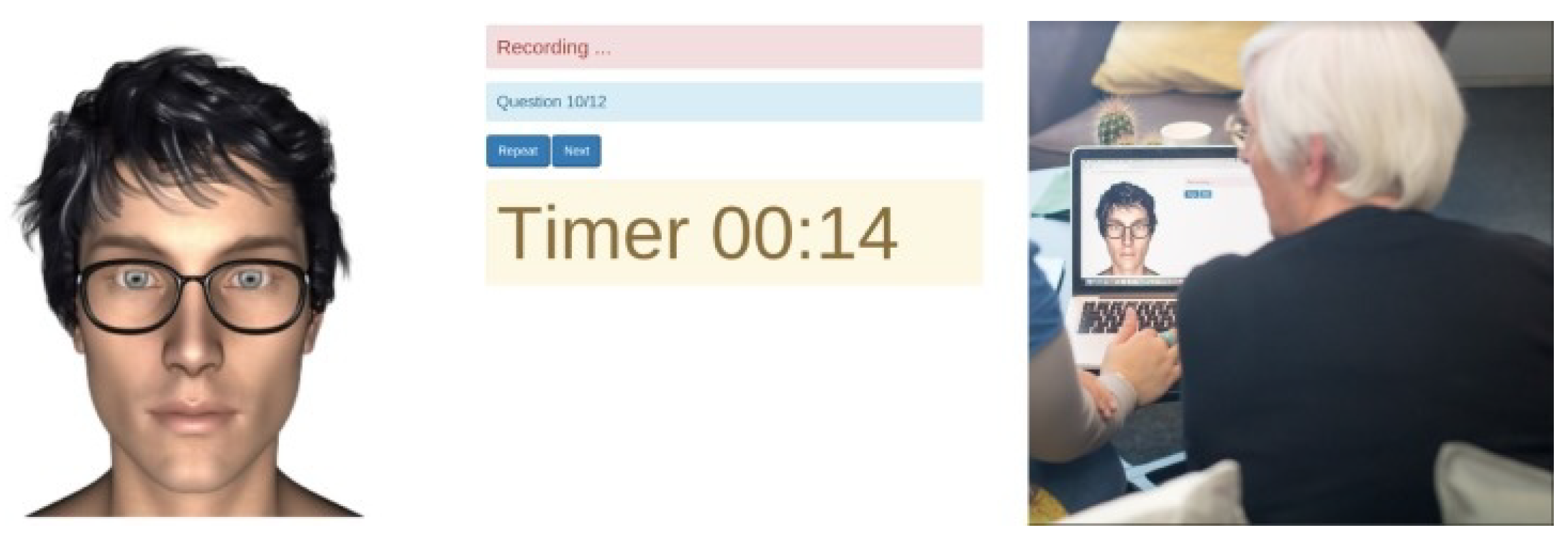
These data include a total of 18 participants who were recorded in 2016, split equally into 6 with ND, 6 with MCI, and 6 with FMD. All participants are in the age range of 43 to 78. The duration of the videos in total is 208 min (mean = 11.56 min). The participants were told that they could bring someone with them and, as a result, 6 of the 18 participants brought an accompanying person with them (4 ND, 1 MCI, and 1 FMD). Therefore, some videos contain four people: the participant, the accompanying person, the neurologist, and the person who operates the laptop (see Figure 1). Although the participants were not given any specific instructions as to where to look, the talking head on the screen will have been the most salient point to look at.

When these data were recorded, it was not intended for video processing purposes, with the intended focus being the audio. Thus, the data contain a high level of noise due to the lack of restrictions on the participants and the environment with respect to the webcam position. We refer to these data as in-the-wild data. They include conditions such as a semi-dark or dark and noisy background (e.g., various objects behind the participant and televisions with animation). Participants could act as they would in their natural environment, such as moving about freely. Participants could continually change the orientation of their faces, rotate their bodies, and move closer to and further away from the camera. Participants wearing glasses occasionally had their eyes obscured by the frames or by reflections from the laptop screen. Also, other people could appear with a participant and move around too. Another aspect was the recording speed for the videos. The majority of the ${\mathrm{IVA}}_{18}$ data recordings were recorded at 30 fps. However, five recordings were recorded at 24 fps, producing a different resolution recording. All these complications cause issues for automatic methods that extract visual information from the data.

3.1.2. ${\mathrm{IVA}}_{34}$ Data

These data were collected in two different environments, a clinic and at home. People at home used laptops and smartphones to carry out the recording. There are 34 videos (19 female and 15 male) representing four groups: 5 participants with ND, 4 with MCI, 2 with FMD, and 23 HCs. The total duration of the videos is 538.59 min (mean = 9.79 min, SD = 5.54 min). Originally, more participants were recorded, but eight were excluded as face detection was difficult due to the following problems: room too dark; interruptions from the participant’s partner; a participant’s eyes not being visible to the camera; two participants wearing masks; the extreme angle of a participant from the smartphone camera; a participant continually looking and talking to the right at the person who was operating the laptop.

As with the ${\mathrm{IVA}}_{18}$ data, in the clinic recordings participants, were told that they could bring someone with them. A total of 4 out of the 13 female participants recorded in a clinic brought a caregiver or partner with them (3 ND and 1 MCI). Consequently, some videos contain four people, as mentioned in the previous section. In contrast, only 2 out of the 20 participants who made a home recording had a caregiver/partner with them during the session (1 MCI and 1 HC).

The use of home environments for recording created many challenges. a participant could choose which room to sit in (e.g., office, living room, bedroom), the distance and the angle from the camera, whether the lights of the room were on or off, and whether to participate in the session during the day or at night time. Rooms chosen could have noisy backgrounds (including furniture such as an office table, or pictures of people, and various objects). In addition, different devices could be used for the recording, e.g., laptops and smartphones. Laptops could be set at any angle with respect to a participant, and the participant could turn their face away from the camera at any time or move out of camera leaving only part of their face visible. Where a smartphone was used, the angle of the camera to the viewer could be continually changing. Smartphone recordings also meant participants generally held the phone and its camera closer to their face and at a lower angle than laptop users, making their head orientation different and their eyes look partially closed. In all cases, people wearing glasses, which was common for the age range captured, also caused challenges.

Although clinic recordings and home recordings share several challenges, the challenge of people appearing with the participant in the camera view is more common in clinic recordings than in home recordings. In the clinic recordings, at least two people appear on camera, as previously mentioned. Taking all of this into account, such data pose a challenge for video-based processing.

In contrast to the ${\mathrm{IVA}}_{18}$ data, the ${\mathrm{IVA}}_{34}$ data include very few participants with health conditions. This makes them less suitable for use in experiments to distinguish between participants with ND, MCI, FMD, and HCs. Therefore, we combined the ${\mathrm{IVA}}_{34}$ data with the ${\mathrm{IVA}}_{18}$ data, which resulted in a larger more balanced dataset with 52 participants, which is referred to as ${\mathrm{IVA}}_{52}$ in the rest of this work. Previous research using the ${\mathrm{IVA}}_{52}$ dataset primarily focused on speech processing [29]. This study is the first to analyze the video recordings from this dataset for cognitive impairment detection.

3.2. Data Pre-Processing

Prior to the feature extraction phase, the IVA videos were pre-processed to deal with other people appearing with a participant in front of the camera. These people were sometimes closer to the camera than the participant. The process was conducted by cropping the height and width of the video frames to detect only the participant while keeping the background noise. The cropping operation resolves only one challenge and does not remove any other challenges to ensure the data can still be considered as in-the-wild. The OpenFace “https://github.com/TadasBaltrusaitis/OpenFace (accessed on 1 February 2020)” toolkit was then used to extract the facial landmarks and head orientation, which is explained in the next section.

3.3. Feature Extraction

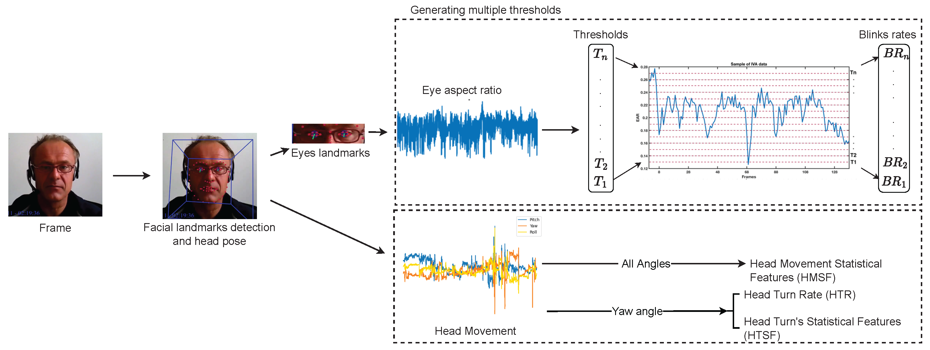
Figure 2 illustrates the complete feature extraction pipeline, which was specifically designed to address the challenges presented by our in-the-wild dataset. This section focuses on extracting three key facial features: eye blink rate (EBR), head turn rate (HTR), and head movement statistical features (HMSFs). HTR measures the frequency of the head turns to the left or right, while HMSFs capture all head movements in any direction. These features are critical behavioral indicators in distinguishing between different CIs and HCs and were chosen based on prior work [5,6].

3.3.1. Eye Blink Rate

The calculation of the EBR is based on the eye aspect ratio (EAR) measure. Six eye landmarks (x,y), where ${\mathit{p}}_1$ and ${\mathit{p}}_4$ represent the horizontal eye corners, and ${\mathit{p}}_2$, ${\mathit{p}}_3$, ${\mathit{p}}_5$ and ${\mathit{p}}_6$ represent the vertical positions of the eyelids, (as shown in Figure 3), were used to compute the EAR according to Equation (1) [30].

$$\mathit{EAR}={\displaystyle \frac{\parallel {\mathit{p}}_2-{\mathit{p}}_6\parallel +\parallel {\mathit{p}}_3-{\mathit{p}}_5\parallel }{2\parallel {\mathit{p}}_1-{\mathit{p}}_4\parallel }}$$

(1)

Both eyes’ EARs are calculated, and then the average is taken. This average EAR is compared with a particular threshold to decide whether there is an eye closure (i.e., the EAR value is lower than the given threshold) or not in each frame. Following [12], a state machine (SM) is used to determine whether an observed eye closure is a genuine blink. The length of the closure is measured in consecutive frames, ranging from 2 to 30 frames. This range allows for variability in the blink duration, as participant tiredness increases during the recording session, leading to longer or more varied eye closure. For example, shorter eye closures may occur early in the session, while longer closures might be observed as the participant becomes fatigued.

The EBR is calculated automatically using an approach based on multiple thresholds (MTs) [12]. The MTs approach calculates the minimum and maximum EAR value over all the participants (OAPs) to generate a range of thresholds for each video. However, the threshold’s upper limit might be dominated by very high EAR values caused by large HMs or turns and occluded faces (i.e., outliers). To address this, any value above the third standard deviation $(\mu +(3\times \sigma \left)\right)$ is considered an outlier and is removed. After the outliers have been removed, different step sizes (0.1, 0.01, and 0.001) are then used to produce the resulting thresholds for the MTs approach. For example, with a minimum of 1 and a maximum of 3, using a step size of 0.1, the thresholds would range from 1.0 to 3.0, resulting in 21 thresholds (1.0, 1.1, 1.2, …, 2.9, 3.0). To account for variation in video length across participants, we normalized all extracted features, including the EBR, based on the number of frames in each video. This ensures comparability and mitigates potential bias due to differing video durations.

In contrast to the previous work that calculated over all participants (MTs) [12], in this work, the MTs approach was developed to become participant-dependent (PD). Thus, MTs-PD calculates the thresholds based on the minimum and maximum for each participant. This approach was chosen to address the issues related to the calculation of the EAR when using the ${\mathrm{IVA}}_{34}$ dataset. Figure 4 shows the mean (blue) and the third SD (orange) of each participant. Notably, the mean and the SD of participants in ${\mathrm{IVA}}_{18}$ are higher than in ${\mathrm{IVA}}_{34}$, which shows that the ${\mathrm{IVA}}_{34}$ participants have a lower range for the EAR than the participants in ${\mathrm{IVA}}_{18}$. The approach that worked for ${\mathrm{IVA}}_{18}$ [25] cannot achieve high performance on the combined ${\mathrm{IVA}}_{52}$ data due to the variations in the recording devices and environments and the other challenges in this dataset (see Section 3.1). Thus, the MTs-PD approach was developed.

As stated previously, the ${\mathrm{IVA}}_{52}$ data include many challenges that resulted in many extremely high values in the EAR. In addition, calculating the mean and the 3rd SD of each participant using the EAR showed a significant difference between the ${\mathrm{IVA}}_{18}$ and the ${\mathrm{IVA}}_{34}$ datasets. As such, the use of the interquartile range (IQR), which is robust in detecting outliers and not sensitive to high values, is considered:

$$IQR=Q3-Q1$$

(2)

$$UB=Q3+b\times IQR$$

(3)

where Q1 and Q3 are the 25th and 75th percentiles of the data, respectively, and a b value of 1.5 is used [31].

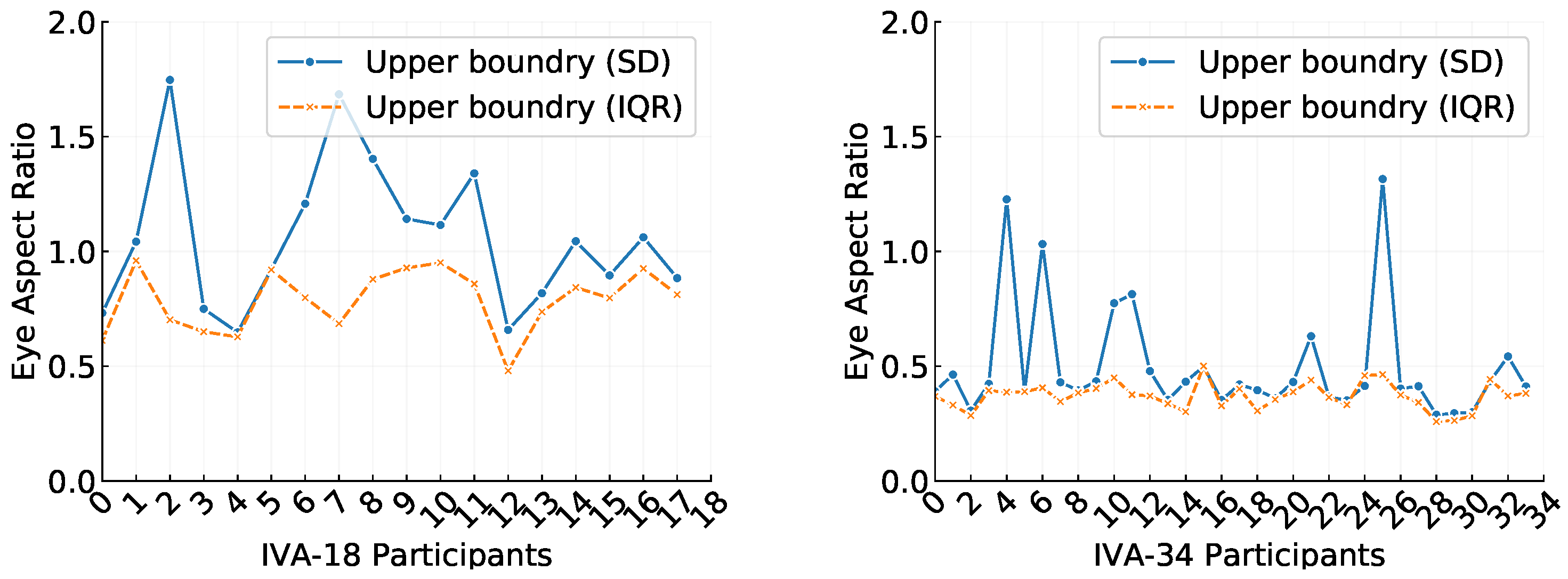
A comparison between the UB of the IQR approach and the 3rd SD approach is shown in Figure 5 for the individual participants in the ${\mathrm{IVA}}_{18}$ and ${\mathrm{IVA}}_{34}$ datasets.

3.3.2. Head Turn Rate

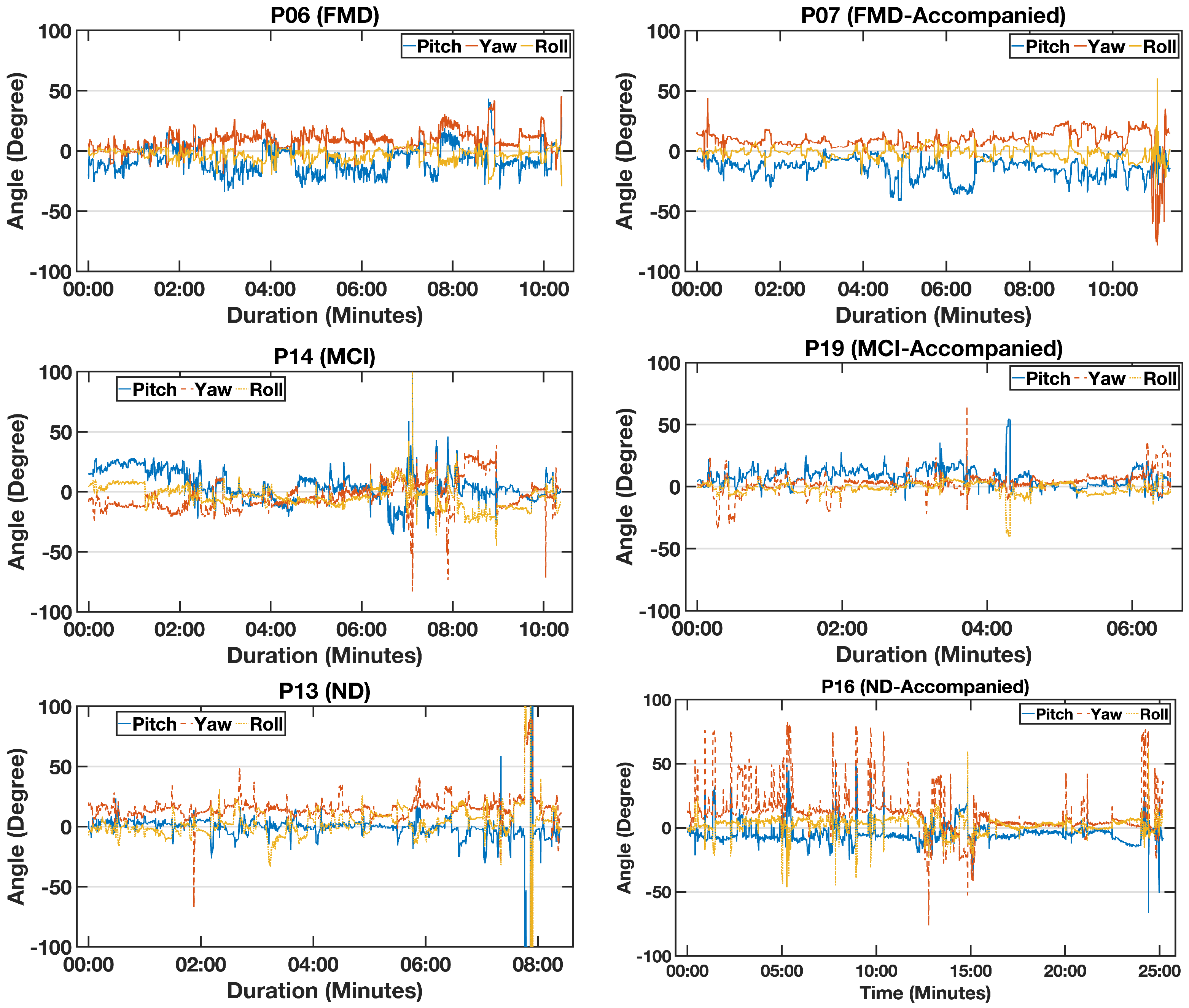
OpenFace was used to extract yaw angles from the videos (see Figure 6). The SciPy (https://docs.scipy.org/doc/scipy/reference/generated/scipy.signal.find_peaks.html, 20 April 2025) package was then used to detect signal peaks, based on a parameter called ‘prominence’, following [25]. Peak prominence measures a peak’s significance based on its intrinsic height and relative location from surrounding peaks. The prominence parameter was set up to find peaks with yaw angle $\pm 45$°. Each detected peak counts as a head turn. The HTR is calculated by dividing the number of head turns by the number of frames. The mean and standard deviation (SD) are then calculated, as well as the variance (Var) for the following derivative features from the detected peaks: peak prominence value, height, width, and distance between peaks. All these statistical features are used as complementary cues with HTR and are referred to as head turn statistical features (HTSFs).

3.3.3. Head Movement

The pitch, yaw, and roll of the head in the videos are used to calculate a range of statistical features (as used in previous work [25,32]). Again, data outliers must be addressed, for example, those caused by extreme HM that are difficult to deal with using OpenFace, as shown in Figure 6 with P14 (MCI) and P13 (ND). The outliers are detected and removed when the value of the pitch, yaw, or roll angle is $\pm 90$°. Then, a linear interpolation process is used to fill in the gaps where outliers occur. Once the interpolation is realized, velocity and acceleration are computed for each angle for each frame. Then, the following statistical features (SFs) for each angle, velocity, and acceleration are calculated and normalized: mean, SD, Var, range, maximum (Max), and minimum (Min). This results in 54 features (6 × 9 features), referred to as HMSFs.

3.4. Fusion

Performance is measured using each feature individually and when fused. The features are fused by concatenating all of them. This study investigates whether feature fusion improves classification performance compared to using a single feature and whether it provides more useful information for small datasets such as the one used in this study.

3.5. Evaluation and Analysis

A range of classification tasks were used in this study: four-way, three-way, and various two-way combinations. Four classifiers were used: support vector machine with linear kernel (SVM), logistic regression (LR), k-nearest neighbor (KNN) with uniform weight, and decision trees (DT). The combined data ${\mathrm{IVA}}_{52}$ include 11 participants with ND, 10 participants with MCI, 8 participants with FMD, and 23 HC participants. The classifiers were trained using the Python 3.11 Scikit-learn package. The classification was participant-independent-stratified k-fold cross-validation. Some hyper-parameter values were optimized using a grid search, and the rest were set to their default values. For each classifier, four metrics were computed: accuracy, recall, precision, and F-measure.

4. Experiments

In this section, we evaluate the performance of our system by analyzing individual features, including the EBR calculation using the MTs-PD approach, head movement features, their fusion, and feature selection.

4.1. Performance Using Eye Blink Features

The MTs-PD approach was developed to address challenges such as the small range of EAR values and the need for a participant-dependent (PD) threshold calculation. Given the variations in the ${\mathrm{IVA}}_{52}$ dataset, including extreme EAR values, we conducted two experiments to evaluate the approach under different conditions.

Experiment 1 evaluates the impact of SD and IQR for outlier removal by varying their factors and assessing performance on three-way (ND vs. MCI vs. FMD) and two-way classification tasks. The two classification tasks include (1) memory problems (MPs) versus HCs, where MP consists of ND, MCI, and FMD, and (2) dementia (ND, MCI) versus non-dementia (FMD, HCs), referred to as D vs. Non-D. Experiment 2 applies the best-performing SD and IQR parameters (factors) from Experiment 1 and extends the evaluation to additional classification tasks, including four-way classification. The following subsections provide a detailed comparison of these approaches.

4.1.1. Experiment 1: Evaluating the Impact of SD and IQR Factor Variations on Classification Performance

In this experiment, two different threshold-scaling factors are explored for both approaches, SD and IQR. These approaches are used to determine the UB for outlier detection within the MTs-PD approach. The factors range from 1 to 3, increasing by increments of 0.5 (i.e., 1, 1.5, 2, 2.5, 3). First, they are investigated via three classification tasks: a three-way problem (ND vs. MCI vs. FMD) and two two-way problems (HC vs. MP) and (HC/FMD vs. ND/MCI). Four different classifiers were investigated, with the KNN classifier achieving the best performance; hence, it was used in subsequent experiments for consistency.

Table 1. Classification results of the three-way problem—neurodegenerative disorder (ND) vs. mild cognitive impairment (MCI) vs. functional memory disorder(FMD)—using a range of values for SD and IQR to find the factor with the highest performance score. These approaches are tested on 70 thresholds.

Factor	Approach	Accuracy	Precision	Recall	F-Measure
1	SD (Min-UB)	44%	31%	40%	32%
	IQR	49%	51%	51%	51%
1.5	SD (Min-UB)	44%	31%	40%	32%
	IQR	53%	58%	53%	52%
2	SD (Min-UB)	44%	31%	40%	32%
	IQR	50%	51%	48%	45%
2.5	SD (Min-UB)	44%	31%	40%	32%
	IQR	53%	58%	53%	52%
3	SD (Min-UB)	44%	31%	40%	32%
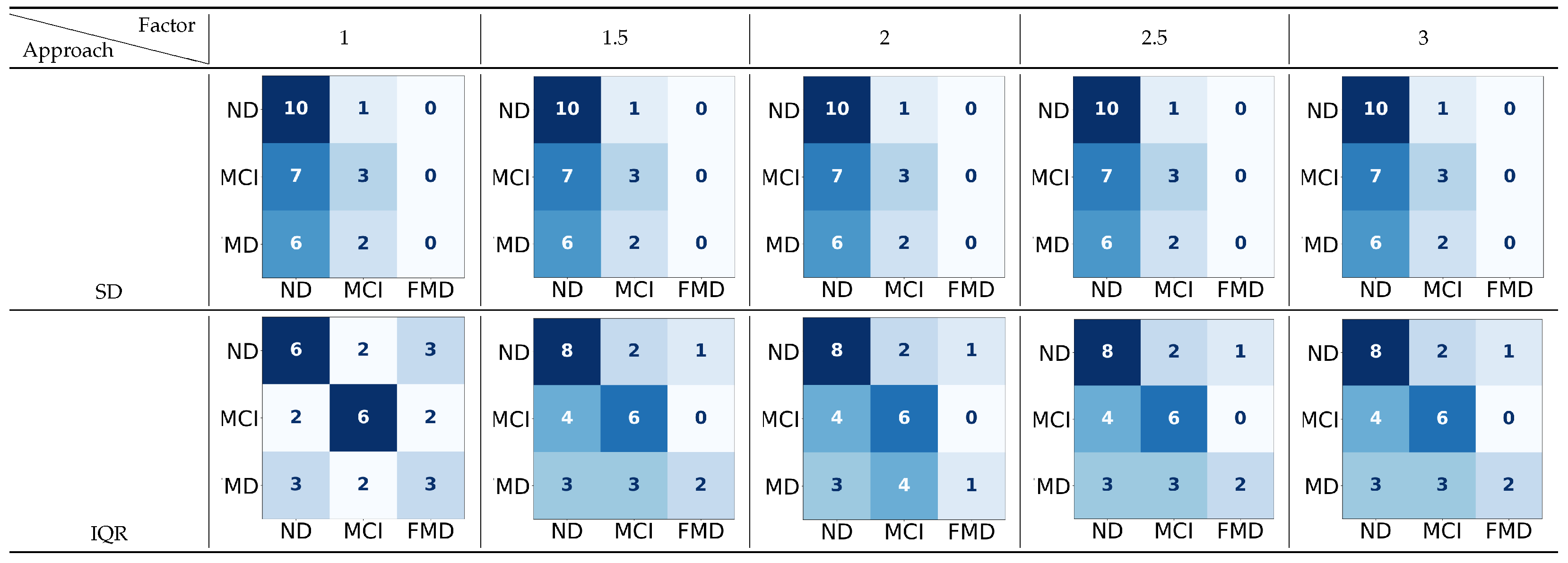
	IQR	53%	58%	53%	52%

presents the results of varying the factor range of the SD and IQR approaches in the three-way classification. The results show that applying IQR to determine the upper boundary improves system performance, unlike SD, which does not improve with factor variation, as illustrated in the confusion matrices in Figure 7. The highest results are obtained with the IQR when factor b equals 1.5, 2.5, and 3. The difference between the IQR and SD results is statistically significant. Similar trends are shown in the two-way classification task (ND/MCI vs. FMD/HCs), as shown in

Table 2. Classification results for the two-way problem—dementia (D) vs. non-dementia (Non-D)—using a range of values for standard deviation (SD) and interquartile range (IQR) to identify the factor that yields the highest performance score. These approaches were evaluated across 70 thresholds or features using k-nearest neighbor (KNN) classification with uniform weighting (D includes MCI and ND).

Factor	Approach	Accuracy	Precision	Recall	F-Measure
1	SD (Min-UB)	63%	62%	59%	58%
	IQR	62%	64%	63%	63%
1.5	SD (Min-UB)	67%	66%	63%	63%
	IQR	71%	72%	71%	71%
2	SD (Min-UB)	64%	64%	62%	62%
	IQR	74%	74%	73%	73%
2.5	SD (Min-UB)	67%	66%	65%	65%
	IQR	71%	72%	71%	71%
3	SD (Min-UB)	64%	64%	61%	61%
	IQR	69%	70%	68%	69%

and Figure 8, where the IQR approach outperforms the SD approach, particularly at factor $b=2$. However, the difference between the SD and IQR results is not statistically significant.

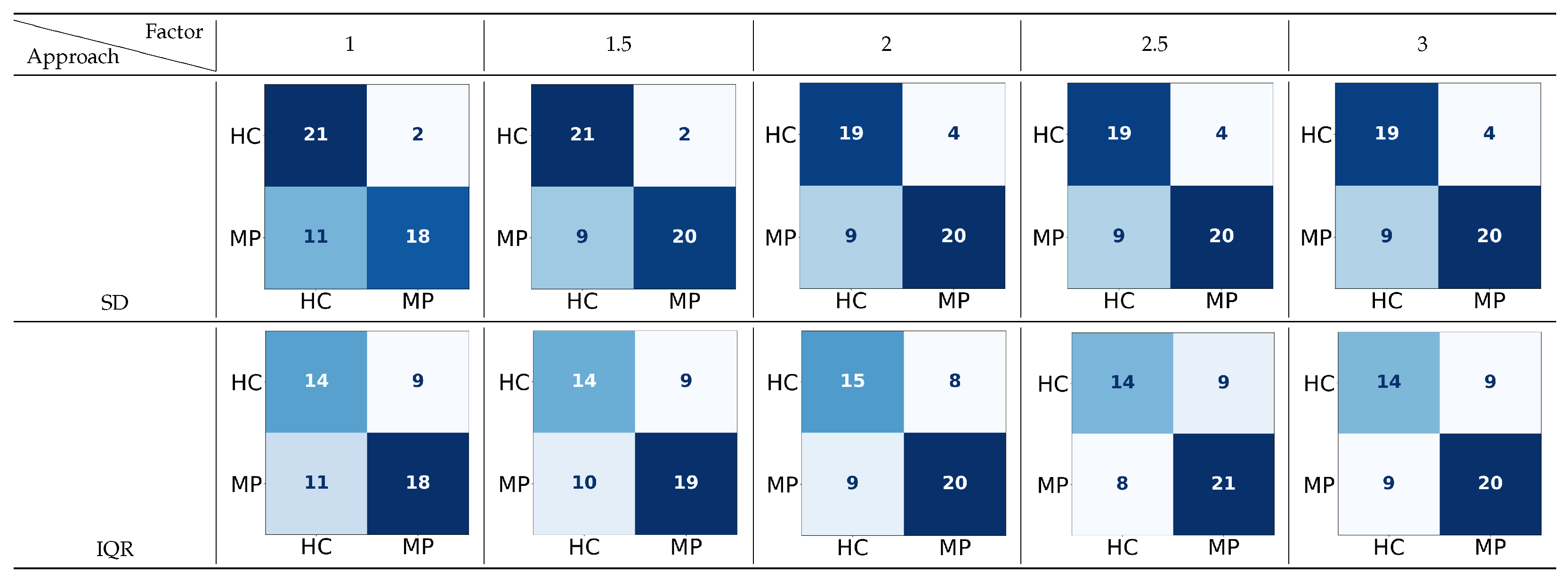
In contrast, the classification task HC vs. MP shows that the SD approach gives a better performance than IQR for all the variations. These findings are different to the results in (ND vs. MCI vs. FMD) and (D vs. Non-D) (see

Table 3. Classification results of the two-way problem—healthy controls (HC) vs. memory problems (MP)—using a range of values for the standard deviation (SD) and interquartile range (IQR) to find the factor with the highest performance score. These approaches are tested on 70 thresholds or features using KNN with uniform weight (MP = includes ND, MCI, and FMD).

Factor	Approach	Accuracy	Precision	Recall	F-Measure
1	SD (Min-UB)	77%	78%	77%	75%
	IQR	63%	61%	61%	61%
1.5	SD (Min-UB)	81%	80%	80%	79%
	IQR	65%	63%	63%	63%
2	SD (Min-UB)	78%	76%	76%	75%
	IQR	69%	67%	67%	67%
2.5	SD (Min-UB)	78%	76%	76%	75%
	IQR	68%	67%	67%	67%
3	SD (Min-UB)	78%	76%	76%	75%
	IQR	68%	68%	67%	67%

and Figure 9). From the table and the confusion matrix, it can be seen that the SD gives the highest performance when it equals 1.5. The difference between the results obtained using SD and IQR is considered to be statistically significant.

From the results shown above, further analysis is needed by investigating the confusion matrices for a specific classification task. The MP vs. HCs classification task was chosen because it includes all groups, and there is a significant performance difference between the IQR and SD results even when their factors are varied. Figure 9 shows that the common misclassified labels are not from a specific dataset (i.e., ${\mathrm{IVA}}_{18}$ or ${\mathrm{IVA}}_{34}$). The incorrect prediction between MP and HC is due to the variation in the recording environments and the devices used. These variations lead to high variations in the range of the EAR calculations that could affect the detection of participants with MP from HC. Interestingly, the HC participants are misclassified when the factor of the SD increases, while the MP participants are correctly classified. For instance, MP participants are classified incorrectly when the factor of the SD is a = 1, although HC participants are classified correctly.

4.1.2. Experiment 2: Extending Classification Evaluation Using Optimal SD and IQR Parameters

We extend the evaluation of the approaches tested in Experiment 1 by applying them to a range of classification tasks: four-way classification (ND vs. MCI vs. FMD vs. HC) and several two-way classifications (ND vs. MCI, ND vs. FMD, MCI vs. FMD, ND vs. HC, MCI vs. HC, FMD vs. HC). These tasks are investigated using both the SD and IQR approaches, with their default factors as well as the factors that achieve the highest performance. The four-way classification results of using both the SD and IQR approaches with their default and optimal factors are shown in

Table 4. Classification results of four-way classification—neurodegenerative disorder (ND) vs. mild cognitive impairment (MCI) vs. functional memory disorder (FMD) vs. healthy controls (HCs)—using two factors for standard deviation (SD) a = 3 as the default value and a = 1.5 as the factor with the highest performance, and for interquartile range (IQR) b = 1.5 as the default value and b = 2 as the factor with the highest performance. These approaches are tested on 70 thresholds (features) using linear SVM.

Factor	Approach	Accuracy	Precision	Recall	F-Measure
a, b = 1.5	SD (Min-UB)	44%	35%	43%	38%
	IQR	49%	53%	49%	49%
a = 3, b = 2	SD (Min-UB)	42%	32%	41%	35%
	IQR	49%	54%	49%	49%

. From Table 4, it can be seen that the IQR achieves the highest performance and that changing the factor shows no difference in the obtained results. It is observed that the detection of participants with MP (e.g., ND vs. MCI, ND vs. FMD, and MCI vs. FMD) is better when the IQR is used. In contrast, the performance decreases when the SD is used, especially for FMD participants classified as HC and MCI. This observation supports the conclusion reached in previous work that classifying FMD participants is challenging even in the clinic [33]. On the other hand, using the SD improves the detection of the HC group from the ND, MCI, and FMD groups. It can be seen that the SD’s UB makes it challenging to distinguish between ND and MCI.

Regarding the two-way classification, the experiment is examined from two aspects: (1) differentiating people with MPs from each other (ND vs. MCI, ND vs. FMD, MCI vs. FMD) and (2) distinguishing each group with MPs from HCs (ND vs. HC, MCI vs. HC, FMD vs. HC). The results of aspect one, classifying individuals with memory-related problems, are presented in

Table 5. Classification results of the two-way classifications—neurodegenerative disorder (ND) vs. mild cognitive impairment (MCI), neurodegenerative disorder (ND) vs. functional memory disorder (FMD), and mild cognitive impairment (MCI) vs. functional memory disorder (FMD)—using two factors for standard deviation (SD), a = 3 as the default value, and a = 1.5 as the factor with highest performance, and for interquartile range (IQR), b = 1.5 as the default value, and b = 2 as the factor with highest performance. These approaches are tested on 70 thresholds or features using linear SVM.

Classes	Approach	Accuracy	Precision	Recall	F-Measure
ND vs. MCI	SD (Min-UB)	67%	68%	67%	66%
	IQR	72%	72%	72%	71%
ND vs. FMD	SD (Min-UB)	56%	29%	50%	37%
	IQR	69%	68%	66%	66%
MCI vs. FMD	SD (Min-UB)	54%	28%	50%	36%
	IQR	67%	70%	64%	63%

. As mentioned above, IQR gives better results in classifying MP classes. The highest performance between the three classification tasks is achieved with 72% to classify ND and MCI from each other. Using the SD causes an incorrect classification for all of the FMD group regardless of the factor value, as presented in Figure 10.

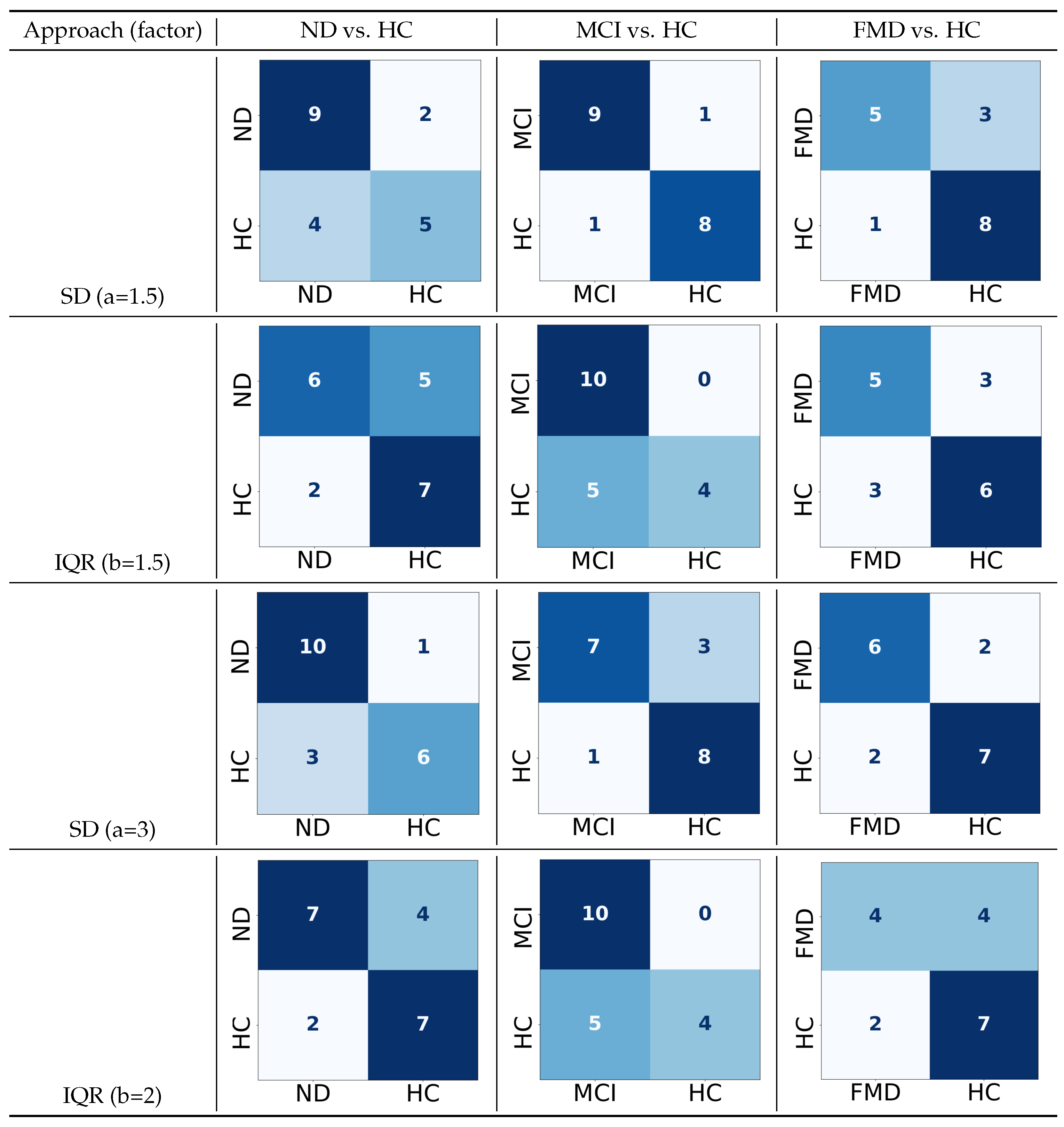
The second aspect of the two-way classification is testing the system performance in classifying every class with MPs from the HC class (ND vs. HC, MCI vs. HC, and FMD vs. HC).

Table 6. Classification results of the two-way classifications—neurodegenerative disorder (ND) vs. healthy controls (HCs), mild cognitive impairment (MCI) vs. healthy controls (HCs), and functional memory disorder (FMD) vs. healthy controls (HCs)—using two factors for standard deviation (SD), a = 3 as the default value, and a = 1.5 as the factor with the highest performance, and for interquartile range (IQR), b = 1.5 as the default value, and b = 2 as the factor with the highest performance. These approaches are tested on 70 thresholds or features using linear SVM (P: precision; R: recall; F1: f-measure).

		ND vs. HC				MCI vs. HC				FMD vs. HC
Factor	Approach	Accuracy	P	R	F1	Accuracy	P	R	F1	Accuracy	P	R	F1
a, b = 1.5	SD (Min-UB)	69%	70%	69%	69%	89%	89%	89%	89%	77%	78%	76%	76%
	IQR	69%	67%	66%	65%	72%	83%	72%	71%	67%	65%	65%	65%
a = 3, b = 2	SD (Min-UB)	78%	81%	79%	79%	78%	80%	79%	79%	77%	76%	76%	76%
	IQR	72%	71%	71%	70%	72%	83%	72%	71%	67%	65%	64%	64%

shows the results of the system performance in each classification task for both approaches and different factor numbers. It can be seen that using the SD approach gives a much better performance than the IQR approach. In ND vs. HC, increasing the threshold range gives better classification performance from factor a = 1.5 with an accuracy of 69% to a = 3 with 78%. In contrast, reducing the threshold range from a = 3 to a = 1.5 enhances the performance from 78% to 89%, respectively. In FMD vs. HC, the SD approach has the same performance when the factor changes. It can be seen in Figure 11 that the predictions of these classes for both approaches explain which class is classified much better. It is observed that using the SD with a high factor (a = 3) increases the detection of ND participants from the HC group.

In contrast, the HC participants could be detected better using IQR regardless of the factor value. Although MCI and HC are detected significantly using the SD with a low factor value (a = 1.5), only two participants are classified incorrectly, as seen in the confusion matrix. Interestingly, it can be seen that none of the MCI participants are ever confused with HC participants when the IQR approach is used.

Regarding the FMD vs. HC classification, the HC participants are much better detected from the FMD group when the SD factor a = 1.5 or 3, and the IQR factor b = 2. The best factor for detecting FMD from HCs is achieved using a high value for the SD factor (a = 3), with only two FMD participants confused with the HC group. Taking all these findings into account, SD with a high factor value could help the model in the training phase to learn by capturing a pattern that could distinguish between these classes with MPs from the HC group. It can be seen that using a low value for the factor results in a model that confuses the two classes and cannot classify them from each other. In contrast, the detection of HC from other classes such as ND and FMD is much better when the IQR is used. It captures a smaller range than the SD, which leads to finding features from the model that identifies the HC from other classes.

When the third quartile of the IQR approach is used to determine the UB, several classification tasks show better performance than when the 3rd SD is used. However, there are also several classification tasks that show better performance when the 3rd SD is used compared to using the IQR approach.

Table 7. All classification tasks and the approach to upper boundary (UB) determination that achieved the highest performance in the t-test to show the significant difference between the highest results obtained using the standard deviation (SD) and interquartile range (IQR) (*: statistically significant; **: extremely statistically significant).

Classification Task	Best IQR or SD?	p-Value
ND vs. MCI vs. FMD vs. HC	IQR	0.04 *
ND vs. MCI vs. FMD	IQR	0.02 *
ND vs. MCI	IQR	0.0003 **
ND vs. FMD	IQR	0.02 *
MCI vs. FMD	IQR	0.03 *
ND vs. HC	SD	0.002 *
MCI vs. HC	SD	0.01 *
FMD vs. HC	SD	0.0004 **
MP vs. HC	SD	0.0001 **
D vs. Non-D	IQR	0.0001 **

summarizes the different classification tasks and which UB-determining approach achieves the best performance with the significance test p-value. The table shows that the IQR approach achieves a better performance on most classification tasks that detect people with MPs (ND/MCI/FMD) and the four-way classification. The difference between the SD and IQR results is considered to be statistically significant. However, the SD approach shows a higher performance when any class of people with MPs is classified from HCs. MCI can be distinguished from HCs better than the ND and FMD groups.

The extracted statistical features of eye blink rate (EBR) from the IVA data can provide valuable insights into behavioral differences between these groups. To investigate this, we conducted a series of statistical significance tests across the ND, MCI, FMD, and HC groups, treated as binary comparisons (ND vs. MCI, ND vs. FMD, MCI vs. FMD, ND vs. HC, MCI vs. HC and FMD vs. HC). First, a normality test was applied to determine whether the features followed a normal distribution. Based on the result, a parametric two-tailed t-test was used for normally distributed features, while a non-parametric Wilcoxon test was used for features that did not meet the normality assumption. A significance level of $p=0.05$ was used for all tests.

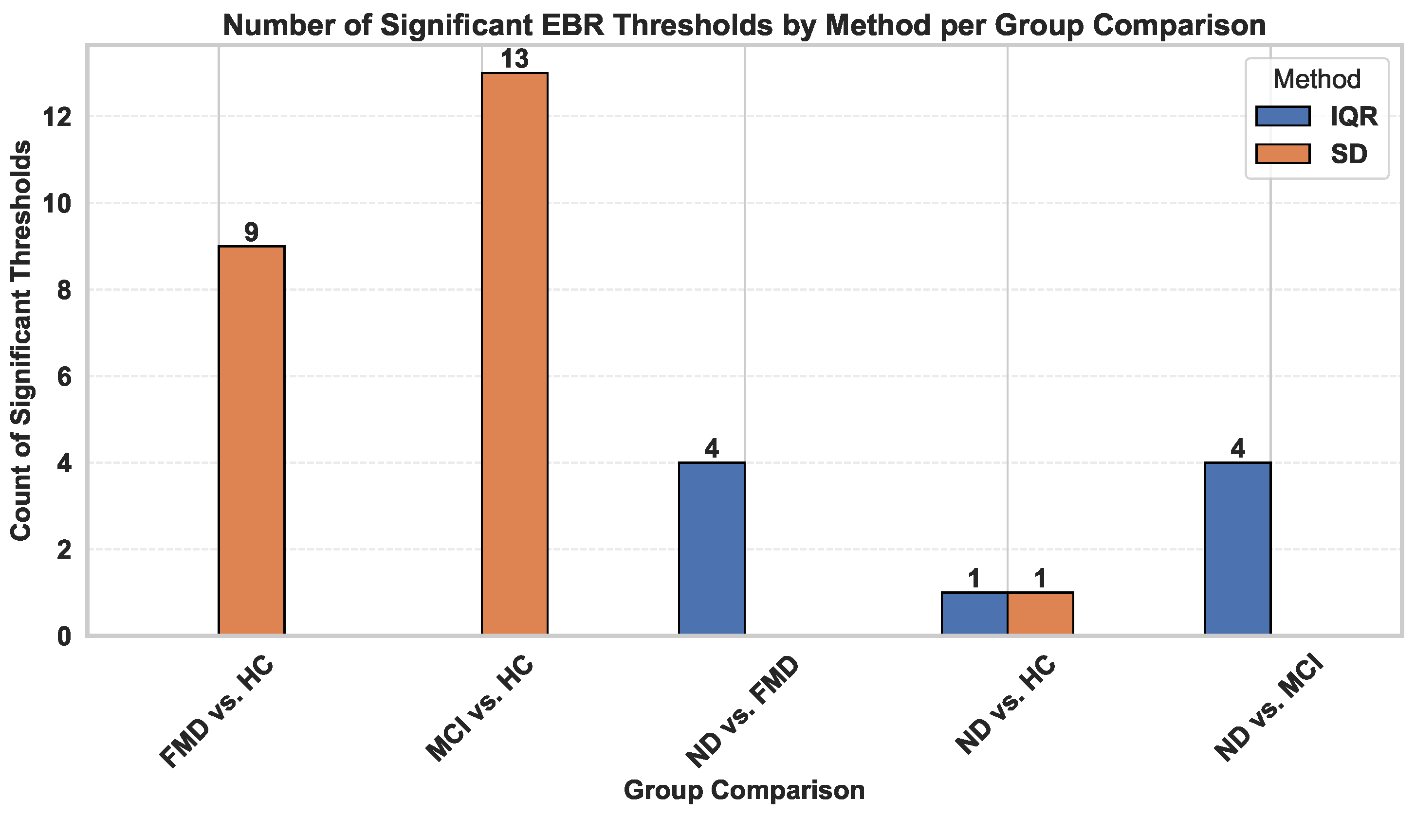
Figure 12 shows the number of statistically significant eye blink rate (EBR) thresholds for each group pair using the two methods: IQR and SD. Each bar represents the count of thresholds that showed significant differences between groups of memory-related problems (ND, MCI, and FMD) and HC. As mentioned previously, the multiple thresholds approach was developed to be participant-dependent (PD), where a range of thresholds is calculated based on the individual minimum and maximum EAR values for each participant. From the chart, it can be seen that some group pairs, such as MCI vs. HC and FMD vs. HC have higher significant thresholds than other group pairs (e.g., ND vs. MCI, ND vs. FMD, and ND vs. HC). This indicates that the differences between these groups are more consistent and noticeable across a wider range of EBR values, suggesting that the EBR feature is more sensitive and reliable for distinguishing between them.

The IQR-based EBR values show statistically significant differences between groups with different memory problems (e.g., ND vs. MCI, ND vs. FMD), but not as consistently between memory problems and healthy controls. This suggests that IQR captures subtle, intra-clinical group differences in EBR behavior, making it more potentially effective for distinguishing between the ND, MCI, and FMD classes.

In contrast, SD-based EBR features demonstrate stronger statistical differences between each memory problem group and the healthy control (HC) group (e.g., ND vs. HC, MCI vs. HC, FMD vs. HC), with many comparisons yielding extremely significant p-values. This supports the observation that using the SD-based method is more effective for tasks that require distinguishing participants with memory problems from healthy controls groups.

These findings confirm and strengthen our earlier interpretation that both the IQR and SD methods serve different yet complementary purposes in eye blink rate (EBR) analysis. The IQR method, by capturing small variations in behavior, performs better when distinguishing between individuals with different memory problems (ND, MCI, FMD). In contrast, the SD method is more effective for differentiating individuals with memory problems from healthy controls, as it reflects larger behavioral differences. This distinction likely arises from varying data characteristics, including recording environments, EAR range shifts, and sample size. In summary, the IQR method is more effective for spotting subtle differences within memory-impaired groups, while the SD method is better suited for distinguishing individuals with memory problems from healthy controls. Future studies should be conducted on larger datasets to further validate these findings.

4.2. Performance Using Head Turns and Movement Features

Head movement (HM) features are evaluated across various classification tasks, including three-way (ND vs. MCI vs. FMD), four-way (ND vs. MCI vs. FMD vs. HC), and multiple two-way classification problems: MP vs. HC, D vs. Non-D, ND vs. MCI, ND vs. FMD, MCI vs. FMD, ND vs. HC, MCI vs. HC, and FMD vs. HC.

Table 8. Classification accuracy of four-way, three-way, and two-way classification tasks for the ${\mathrm{IVA}}_{52}$ dataset, measuring the system performance using individual features with the KNN classifier. The number of features is indicated in parentheses.

Classification Task	Feature	Accuracy	Precision	Recall	F-Measure
ND/MCI/FMD/HC	HTR (1)	45%	46%	42%	59%
	HTR + HTSF (13)	48%	50%	46%	53%
	HMSF (54)	44%	45%	44%	44%
ND/MCI/FMD	HTR (1)	45%	31%	46%	37%
	HTR + HTSF (13)	59%	60%	58%	58%
	HMSF (54)	53%	59%	55%	53%
ND/MCI	HTR (1)	53%	51%	51%	46%
	HTR + HTSF (13)	52%	52%	50%	69%
	HMSF (54)	62%	62%	62%	62%
ND/FMD	HTR (1)	73%	76%	70%	71%
	HTR + HTSF (13)	92%	89%	89%	89%
	HMSF (54)	69%	68%	66%	66%
MCI/FMD	HTR (1)	71%	72%	73%	72%
	HTR + HTSF (13)	67%	71%	69%	66%
	HMSF (54)	90%	92%	88%	88%
MP/HC	HTR (1)	72%	71%	71%	71%
	HTR+HTSF (13)	64%	63%	62%	62%
	HMSF (54)	73%	73%	72%	72%
D/Non-D	HTR (1)	69%	66%	64%	64%
	HTR + HTSF (13)	75%	72%	71%	72%
	HMSF (54)	73%	70%	70%	70%
ND/HC	HTR (1)	83%	85%	84%	85%
	HTR + HTSF (13)	72%	77%	73%	73%
	HMSF (54)	74%	75%	74%	74%
MCI/HC	HTR (1)	74%	74%	74%	74%
	HTR + HTSF (13)	69%	68%	68%	68%
	HMSF (54)	69%	68%	68%	68%
FMD/HC	HTR (1)	67%	65%	64%	64%
	HTR + HTSF (13)	45%	25%	44%	32%
	HMSF (54)	58%	59%	58%	58%

presents the classification accuracy results for these tasks.

The results indicate that HTR and its derivative features (HTR + HTSF) are informative for classification. However, distinguishing FMD from HCs remains the most challenging task. The highest classification accuracy is achieved using HTR + HTSF features, with 59% and 48% accuracy for the three-way and four-way classification tasks, respectively. Additionally, this feature set achieves 92% accuracy in ND vs. FMD classification and 75% in D vs. Non-D classification.

Moreover, HMSFs prove useful in distinguishing groups with overlapping characteristics, achieving 62% accuracy in ND vs. MCI classification and 90% in MCI vs. FMD classification. In contrast, HTR+HTSF features excel in differentiating groups with more distinct characteristics, such as in three-way, four-way, and two-way (ND vs. FMD and D vs. Non-D) classifications.

Certain features perform better in specific two-way tasks. For instance, HTR + HTSF achieves 92% accuracy in ND vs. FMD classification, while the HTR feature alone achieves 72% accuracy in MCI vs. FMD classification. When classifying individuals with memory-related problems against HCs, HTR provides the best performance, with classification accuracies of 83% for ND vs. HC, 74% for MCI vs. HC, and 67% for FMD vs. HC. These findings align with previous research [6,34,35,36], which suggests that individuals with ND tend to exhibit more head movement due to the presence of an accompanying person.

4.3. Performance by Feature Fusion

The results obtained from feature fusion are presented in

Table 9. Classification accuracy of four-way, three-way, and two-way classification tasks for the ${\mathrm{IVA}}_{52}$ dataset, measuring the system performance using the interquartile range (IQR) approach as the upper boundary (UB) when features are fused and selected with the KNN classifier. The number of features is indicated in parentheses.

Classification Task	Feature	Accuracy	Precision	Recall	F-Measure
ND/MCI/FMD/HC	Feature fusion (137)	44%	44%	46%	44%
	Feature selection (5)	32%	26%	30%	28%
ND/MCI/FMD	Feature fusion (137)	48%	47%	46%	46%
	Feature selection (5)	43%	50%	45%	42%
ND/MCI	Feature fusion (137)	75%	84%	75%	74%
	Feature selection (6)	63%	63%	61%	60%
ND/FMD	Feature fusion (137)	73%	73%	74%	73%
	Feature selection (20)	76%	78%	78%	78%
MCI/FMD	Feature fusion (137)	65%	70%	64%	63%
	Feature selection (7)	52%	49%	49%	49%
MP/HC	Feature fusion (137)	62%	61%	61%	61%
	Feature selection (116)	59%	67%	57%	57%
D/Non-D	Feature fusion (137)	70%	68%	68%	68%
	Feature selection (37)	62%	59%	59%	59%
ND/HC	Feature fusion (137)	85%	85%	84%	85%
	Feature selection (38)	60%	65%	64%	63%
MCI/HC	Feature fusion (137)	72%	74%	74%	74%
	Feature selection (38)	60%	65%	64%	63%
FMD/HC	Feature fusion (137)	79%	78%	76%	76%
	Feature selection (2)	47%	47%	47%	47%

. The IQR approach is used for simplicity and because it provides the highest performance results in most cases. Feature fusion generally improves performance compared to individual features. However, for the three-way and four-way classification tasks, performance remains similar to using individual features, showing no significant improvement.

In comparing SD and IQR as UBs, SD generally shows lower performance, particularly in classification tasks that distinguish between individuals with memory problems (ND/MCI, ND/FMD, MCI/FMD, and ND/MCI/FMD). In contrast, the IQR approach usually provides better results when classifying individuals with memory problems from HCs.

4.4. Performance by Feature Selection

Table 9 presents the results when applying feature selection, where only the most relevant features are retained. This generally did not improve performance for most classification tasks, except for cases like ND/MCI. The IQR method performs better in most classification tasks, particularly in distinguishing between memory problem classes, including three-way, four-way, and D/Non-D classification tasks. This suggests that using the full feature dimension is necessary to achieve better performance.

Moreover, it can be seen that conducting the classification task between two classes that are close to each other, such as MCI/FMD, shows a decrease in the performance because this task is also difficult for doctors to distinguish between in the hospital [33].

These findings highlight the key difference between feature fusion and feature selection. While feature fusion leverages complementary information from multiple features to improve performance, particularly in distinguishing between distinct groups, feature selection often reduces performance by discarding potentially useful features. This is especially evident in tasks with overlapping classes, such as MCI vs. FMD, where removing features can lead to a loss of crucial discriminative information. However, in specific cases like ND vs. MCI, feature selection provides a slight improvement, suggesting that certain features may contribute more effectively to distinguishing between particular memory problem groups.

4.5. Comparison with Previous Work

This section compares our results with related work that used either visual or audiovisual modalities, as shown in

Table 10. Classification results (%) for dementia detection compared to previous work.

Study	Participants	Data Settings	Modality	Classifier	Performance
[10]	18 (9 with dementia)	Lab-controlled	Audiovisual	SVM	84%
[7]	29 (14 with dementia including (NPH, AD, DLB, MCI))	Lab-controlled	Audiovisual	LR	93%
[8]	24 (12 with dementia)	Lab-controlled	Visual	LR	82%
[12]	${\mathrm{IVA}}_{18}$ (6 ND, 6 MCI, and 6 FMD)	In-the-wild	Visual	SVM	89%
[25]	${\mathrm{IVA}}_{18}$ (6 ND, 6 MCI, and 6 FMD)	In-the-wild	Visual	SVM	78%
[11]	32 videos (MCI and HCs)	Semi-in-the-wild	Visual	DL	87%
Our	${\mathrm{IVA}}_{52}$ (29 MP, 23 HCs)	In-the-wild	Visual	KNN	59%
	${\mathrm{IVA}}_{52}$ subset (11 ND, 10 MCI, and 8 FMD)	In-the-wild	Visual	KNN	81%
	${\mathrm{IVA}}_{52}$ subset (10 MCI, 9 HCs)	In-the-wild	Visual	KNN	89%

. The performance column in the table represents the classification accuracy achieved in each study. The findings demonstrate that the performance achieved in our work is comparable to that in prior studies that employed visual or audiovisual features.

Prior work such as [7,8,10] used datasets recorded in lab-controlled environments. Work that used audiovisual features with the smile as the facial feature achieved accuracies of 84% using SVM and 93% using LR [7,10]. However, their work was limited to Japanese people because they used a Japanese female model to extract the smile feature. Later work employing only visual features, including facial action units, eye gaze, and lip activity, achieved an accuracy of 82% using LR [8]. In contrast, our work is based on a dataset recorded in the wild, as described in Section 3.1, which introduces additional challenges such as variable lighting, background noise, and participant movement.

Another key difference is the classification tasks. Prior studies primarily focused on detecting dementia from HCs regardless of the dementia type even though their dementia group includes several dementia types such as Alzheimer’s disease (AD), MCI, normal pressure hydrocephalus, and dementia with Lewy bodies (DLB) [7,8,10]. Other work focused only on detecting MCI from HCs [11]. Our work focused on investigating different memory-related conditions (ND, MCI, FMD) both from each other and from HCs, across a range of classification tasks.

A recent study employed neural networks (NNs) to extract facial features, achieving 87% accuracy in distinguishing MCI from HCs [11]. However, their dataset consisted of video-recorded, semi-structured interviews where participants were clearly visible, and lighting conditions were optimal. In contrast, we utilized hand-crafted features (HCFs) instead of NNs, as HCFs require less training data while still achieving comparable results with an accuracy of 89%.

Finally, Table 10 includes results obtained using the ${\mathrm{IVA}}_{18}$ dataset [12,25] and the ${\mathrm{IVA}}_{52}$ dataset (the row labeled ‘Our’). The results show that the performance tends to decrease when using the ${\mathrm{IVA}}_{52}$ dataset, which is probably due to the increased variability and complexity of the in-the-wild recordings.

5. Discussion

As seen in the previous section, feature fusion shows better results than feature selection. A possible explanation for this could be that every feature contributes to differentiating groups from each other. For a better understanding of the results obtained, an analysis was conducted using a confusion matrix.

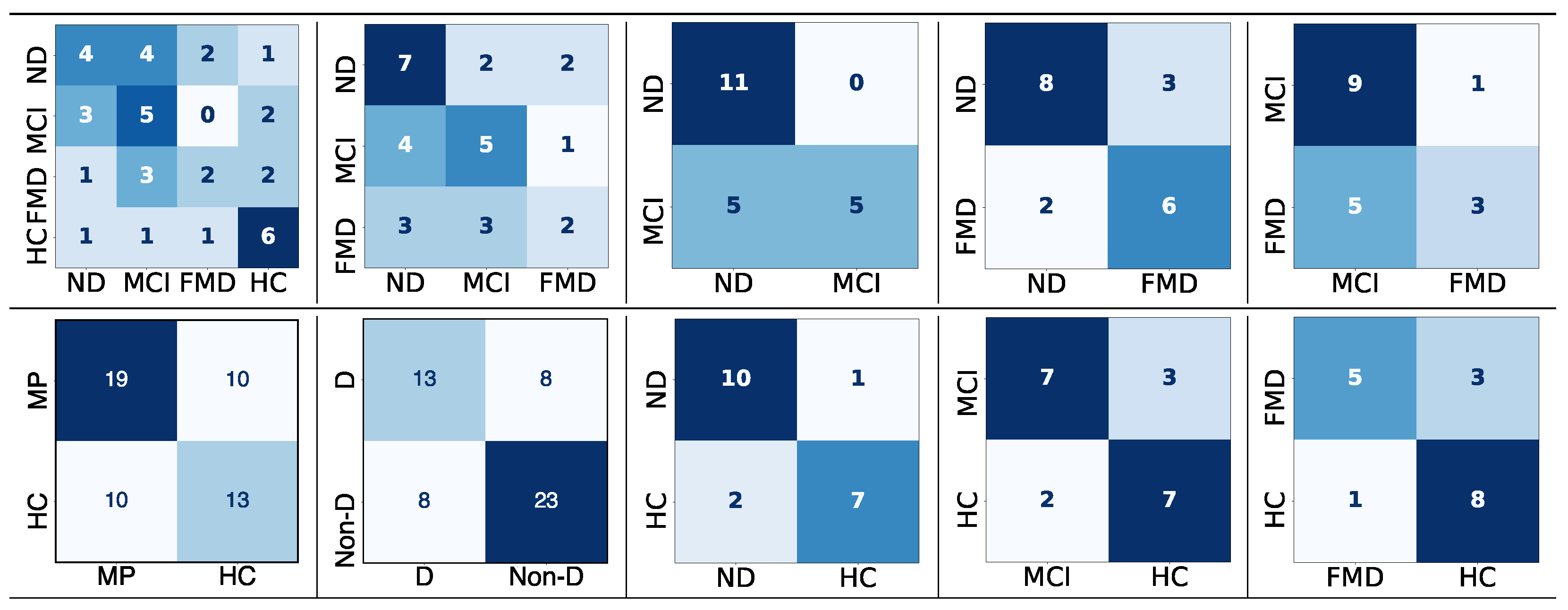
Figure 13 shows the confusion matrices for all the classification tasks using the IQR approach to detect the UB—IQR was chosen because it provided better results than the SD approach for most of the classification tasks. It can be seen that ND and MCI are misclassified as MCI and ND, respectively, in the four-way classification task due to the overlap between these groups. Another reason is that ND participants who were misclassified as MCI attended the session alone, whereas MCI participants who were misclassified as ND attended with a partner/caregiver. In addition, another source of confusion can be seen in FMD participants, who were mostly classified as MCI in the four-way, three-way, and two-way classifications tasks. The reason behind this confusion is due to the existing overlap between these groups, which makes it a very challenging task, consistent with previous findings [33].

From Figure 13, it is apparent that there is a significant difference between the following conditions when predicted using the selected HC participants who only used a laptop as a recording device and were in environmental conditions similar to other groups: ND/HC, MCI/HC, and FMD/HC. Even in the four-way classification task, most of the HC participants are correctly classified. On the other hand, for MP/HC groups and D/Non-D groups, the misclassified participants are not limited to a particular class; instead, misclassification is related to variations in the recording environments and the devices used.

These findings suggest that these possible sources of error could have been caused by the lack of diagnostic details regarding the type of dementia that participants have. Certain types of dementia, such as vascular dementia (VaD) and DLB, may not exhibit a head turn cue [35], which could contribute to misclassification. Including more diagnostic information is essential for improving error analysis and developing an automatic tool to handle overlapping conditions, such as AD, VaD, DLB, and behavioral-variant frontotemporal dementia (FTD).

Looking more closely at the interaction between sex, age and whether a partner is present is of interest. Refs. [6,37] suggested that ‘attending with’ is an additional cue to the head turn due to its effect on the latter. In the ${\mathrm{IVA}}_{52}$ dataset, the number of participants who came with a partner is 12 participants (7 ND, 3 MCI, 1 FMD, 1 HC). The data show that participants who came with a partner generally show significant head turns and movements, which is consistent with related work findings [6,38]. Moreover, they suggested that the presence of head turn indicates CI and AD. In contrast, Ref. [35] found that the presence of the head turn cue indicates CI whether the participant attended with a partner or came alone. The findings of this research, while preliminary, seem to be consistent with other research, which found that increases in EBR and head turn or movements can indicate a higher risk of progression to AD [5,38]. It is also assumed that sex and age may play a vital role in the HTR.

In the ${\mathrm{IVA}}_{18}$ data, all of the female participants came with a partner regardless of their diagnostic class, whilst only two males from the ND class came with partners. Moreover, in the ${\mathrm{IVA}}_{34}$ data, all the female participants who came with partners have health conditions, but only two males from the MCI and HC classes came with a partner. Ref. [35] investigated the severity and the incidence of the head turn cue on 125 patients by observing whether the patients showed a head turn cue during a cognitive test and found that the females tended to bring a partner. Their findings showed that women find it easier to depend on someone else when they face difficulties, whereas men feel obligated to deal with difficulties without help. Previous work compared men and women with CI in terms of the prevalence of behavioral symptoms and found that ‘help seeking’ and depression are more frequent in women [39]. However, men showed more regressive and aggressive behaviours than women. These findings contradict those of previous work that found partner presence to be independent of sex [36,40] but dependent on age [22]. Moreover, Ref. [40] reported that head turn indicates a CI regardless of sex or age. However, there is no information on whether these factors are affected by other external factors such as culture.

To fully assess the clinical applicability and generalizability of the proposed system, future work should include validation on larger and more diverse multi-center datasets. Moreover, benchmarking the method against state-of-the-art deep learning models—which have shown strong potential in similar applications—will be essential for evaluating its scalability and practical relevance in real-world clinical settings. Although deep learning approaches typically require larger datasets, recent developments in video-based cognitive assessment, using architectures such as convolutional neural networks (CNNs) and transformers, show considerable promise and should be explored as complementary or alternative methods. Further work is also needed to systematically quantify how environmental factors such as lighting variability, camera angle, or background clutter affect classification accuracy.

While our method is designed for naturalistic “in-the-wild” settings—capturing real-world variation in participants’ behavior and environment—this very complexity introduces challenges that can negatively impact classification performance. The variability in lighting, camera positioning, background stimuli, and participant compliance may introduce noise or inconsistencies in the extracted features. This may partly explain why the classification accuracy is more modest compared to studies using controlled lab environments.

In this context, it is worth noting that participants in our study completed tasks in varied home environments, introducing potential differences in lighting, background, and incidental stimuli that could influence feature extraction. We acknowledge that these factors may limit the reliability and consistency of certain features, such as head movement or eye behavior, under uncontrolled conditions. Future work should examine the impact of such variability and explore strategies to control for or model these environmental factors. Beyond technical validation, future research should also investigate how this technology could be realistically integrated into clinical workflows, for example, as an adjunct screening tool in memory clinics to support remote cognitive assessments.

6. Conclusions

Unlike traditional methods that rely on controlled environments and subjective assessments, this work demonstrates the feasibility of an automated and accessible screening tool for dementia detection in real-world settings. This study investigated facial cues—eye blink rate (EBR) and head movement (HM) features—as reliable indicators of CI in in-the-wild conditions, individually and fused.

In this work, we improve on the MTs approach for EBR calculation, enhancing its robustness for real-world applications. Our results show that EBR remains a reliable CI indicator in in-the-wild settings. Additionally, we investigate the role of HM features in video-based dementia detection, using a larger dataset for the first study of its kind. This dataset consists of ND, MCI, FMD, and HC participants. Our findings show that HM features enhance classification performance beyond using EBR alone, and their fusion further improves results, highlighting their combined effectiveness. In this work, we achieved promising results using an in-the-wild dataset, comparable to results in previous work that uses controlled datasets.

Furthermore, this study demonstrates that a visual-only approach can achieve competitive accuracy compared to multimodal methods, reinforcing its potential as a scalable and cost-effective diagnostic tool. However, a key limitation of this study is the small sample size, which may affect the generalizability of the findings. Despite this, the results suggest that behavioral features hold promise for future applications in home-based assessments. With further work, including a larger dataset and additional features, such as facial expressions and speech, this approach could be refined to enhance its robustness and applicability in real-world settings.

References

1. Mavrodaris, A.; Powell, J.; Thorogood, M. Prevalences of dementia and cognitive impairment among older people in sub-Saharan Africa: A systematic review. Bull. World Health Organ. 2013, 91, 773–783. [Google Scholar] [CrossRef] [PubMed]
2. World Health Organization. Risk Reduction of Cognitive Decline and Dementia: WHO Guidelines; World Health Organization: Geneva, Switzerland, 2019. [Google Scholar]
3. Rosenzweig, A. Montreal Cognitive Assessment (MoCA) Test for Dementia. Verywell Health. 2025. Available online: https://www.verywellhealth.com/alzheimers-and-montreal-cognitive-assessment-moca-98617 (accessed on 31 May 2025).
4. Richmond, V.P.; McCroskey, J.C.; Hickson, M. Nonverbal Behavior in Interpersonal Relations; Allyn & Bacon: Boston, MA, USA, 2008. [Google Scholar]
5. Ladas, A.; Frantzidis, C.; Bamidis, P.; Vivas, A.B. Eye blink rate as a biological marker of mild cognitive impairment. Int. J. Psychophysiol. 2014, 93, 12–16. [Google Scholar] [CrossRef] [PubMed]
6. Larner, A. Head turning sign: Pragmatic utility in clinical diagnosis of cognitive impairment. J. Neurol. Neurosurg. Psychiatry 2012, 83, 852–853. [Google Scholar] [CrossRef] [PubMed]
7. Tanaka, H.; Adachi, H.; Ukita, N.; Ikeda, M.; Kazui, H.; Kudo, T.; Nakamura, S. Detecting dementia through interactive computer avatars. IEEE J. Transl. Eng. Health Med. 2017, 5, 1–11. [Google Scholar] [CrossRef]
8. Tanaka, H.; Adachi, H.; Kazui, H.; Ikeda, M.; Kudo, T.; Nakamura, S. Detecting dementia from face in human-agent interaction. In Proceedings of the Adjunct of the 2019 International Conference on Multimodal Interaction, Suzhou, China, 14–18 October 2019; pp. 1–6. [Google Scholar]
9. Murphy, D.; Ni Loingsigh, A.; Bernie, I.; Bak, T.H. Bilingualism and dementia: How some patients lose their second language and rediscover their first. Lang. Vic. 2019, 23, 81–83. [Google Scholar]
10. Tanaka, H.; Adachi, H.; Ukita, N.; Kudo, T.; Nakamura, S. Automatic detection of very early stage of dementia through multimodal interaction with computer avatars. In Proceedings of the 18th ACM International Conference on Multimodal Interaction, Tokyo Japan, 12–16 November 2016; pp. 261–265. [Google Scholar]
11. Alsuhaibani, M.; Dodge, H.H.; Mahoor, M.H. Mild cognitive impairment detection from facial video interviews by applying spatial-to-temporal attention module. Expert Syst. Appl. 2024, 252, 124185. [Google Scholar] [CrossRef]
12. Alzahrani, F.; Mirheidari, B.; Blackburn, D.; Maddock, S.; Christensen, H. Eye Blink Rate Based Detection of Cognitive Impairment Using In-the-wild Data. In Proceedings of the 2021 9th International Conference on Affective Computing and Intelligent Interaction (ACII), Nara, Japan, 28 September–1 October 2021; pp. 1–8. [Google Scholar]
13. Jongkees, B.J.; Colzato, L.S. Spontaneous eye blink rate as predictor of dopamine-related cognitive function—A review. Neurosci. Biobehav. Rev. 2016, 71, 58–82. [Google Scholar] [CrossRef]
14. von Cramon, D.; Schuri, U. Blink frequency and speech motor activity. Neuropsychologia 1980, 18, 603–606. [Google Scholar] [CrossRef]
15. Beck, A.T.; Steer, R.A.; Ball, R.; Ranieri, W.F. Comparison of Beck Depression Inventories-IA and-II in psychiatric outpatients. J. Personal. Assess. 1996, 67, 588–597. [Google Scholar] [CrossRef]
16. De Jong, P.J.; Merckelbach, H. Eyeblink frequency, rehearsal activity, and sympathetic arousal. Int. J. Neurosci. 1990, 51, 89–94. [Google Scholar] [CrossRef]
17. Argilés, M.; Cardona, G.; Pérez-Cabré, E.; Rodríguez, M. Blink rate and incomplete blinks in six different controlled hard-copy and electronic reading conditions. Investig. Ophthalmol. Vis. Sci. 2015, 56, 6679–6685. [Google Scholar] [CrossRef] [PubMed]
18. Sun, W.S.; Baker, R.S.; Chuke, J.C.; Rouholiman, B.R.; Hasan, S.A.; Gaza, W.; Stava, M.W.; Porter, J.D. Age-related changes in human blinks. Passive and active changes in eyelid kinematics. Investig. Ophthalmol. Vis. Sci. 1997, 38, 92–99. [Google Scholar]
19. Mota, I.A.; Lins, O.G. Bereitschaftspotential preceding spontaneous and voluntary eyelid blinks in normal individuals. Clin. Neurophysiol. 2017, 128, 100–105. [Google Scholar] [CrossRef] [PubMed]
20. Woodruff-Pak, D.S. Eyeblink classical conditioning differentiates normal aging from Alzheimer’s disease. Integr. Physiol. Behav. Sci. 2001, 36, 87–108. [Google Scholar] [CrossRef]
21. Chen, W.; Chiang, T.; Hsu, M.; Liu, J. The validity of eye blink rate in Chinese adults for the diagnosis of Parkinson’s disease. Clin. Neurol. Neurosurg. 2003, 105, 90–92. [Google Scholar] [CrossRef]
22. Larner, A.J. Dementia in Clinical Practice: A Neurological Perspective: Pragmatic Studies in the Cognitive Function Clinic; Springer: London, UK, 2014. [Google Scholar]
23. Fraser, K.C.; Lundholm Fors, K.; Eckerström, M.; Öhman, F.; Kokkinakis, D. Predicting MCI status from multimodal language data using cascaded classifiers. Front. Aging Neurosci. 2019, 11, 205. [Google Scholar] [CrossRef]
24. Barral, O.; Jang, H.; Newton-Mason, S.; Shajan, S.; Soroski, T.; Carenini, G.; Conati, C.; Field, T. Non-Invasive classification of Alzheimer’s disease using eye tracking and language. In Proceedings of the Machine Learning for Healthcare Conference, Virtual, 7–8 August 2020; pp. 813–841. [Google Scholar]
25. Alzahrani, F.; Mirheidari, B.; Blackburn, D.; Maddock, S.; Christensen, H. Investigating Visual Features for Cognitive Impairment Detection Using In-the-wild Data. In Proceedings of the 2023 IEEE 17th International Conference on Automatic Face and Gesture Recognition (FG), Waikoloa Beach, HI, USA, 5–8 January 2023; pp. 1–8. [Google Scholar]
26. Poor, F.F.; Dodge, H.H.; Mahoor, M.H. A multimodal cross-transformer-based model to predict mild cognitive impairment using speech, language and vision. Comput. Biol. Med. 2024, 182, 109199. [Google Scholar] [CrossRef]
27. Mirheidari, B.; Blackburn, D.; Harkness, K.; Walker, T.; Venneri, A.; Reuber, M.; Christensen, H. An avatar-based system for identifying individuals likely to develop dementia. In Proceedings of the Interspeech 2017, Stockholm, Sweden, 20–24 August 2017; pp. 3147–3151. [Google Scholar]
28. Mirheidari, B.; Blackburn, D.; Walker, T.; Venneri, A.; Reuber, M.; Christensen, H. Detecting Signs of Dementia Using Word Vector Representations. In Proceedings of the Interspeech, Hyderabad, India, 2–6 September 2018; pp. 1893–1897. [Google Scholar]
29. Mirheidari, B.; Blackburn, D.; Walker, T.; Reuber, M.; Christensen, H. Dementia detection using automatic analysis of conversations. Comput. Speech Lang. 2019, 53, 65–79. [Google Scholar] [CrossRef]
30. Soukupova, T.; Cech, J. Eye blink detection using facial landmarks. In Proceedings of the 21st Computer Vision Winter Workshop, Rimske Toplice, Slovenia, 3–5 February 2016. [Google Scholar]
31. Simmons, J.P.; Nelson, L.D.; Simonsohn, U. False-positive psychology: Undisclosed flexibility in data collection and analysis allows presenting anything as significant. Psychol. Sci. 2011, 22, 1359–1366. [Google Scholar] [CrossRef]
32. Alghowinem, S.; Goecke, R.; Wagner, M.; Parkerx, G.; Breakspear, M. Head pose and movement analysis as an indicator of depression. In Proceedings of the 2013 Humaine Association Conference on Affective Computing and Intelligent Interaction, Geneva, Switzerland, 2–5 September 2013; pp. 283–288. [Google Scholar]
33. Wakefield, S.J.; Blackburn, D.J.; Harkness, K.; Khan, A.; Reuber, M.; Venneri, A. Distinctive neuropsychological profiles differentiate patients with functional memory disorder from patients with amnestic-mild cognitive impairment. Acta Neuropsychiatr. 2018, 30, 90–96. [Google Scholar] [CrossRef]
34. Larner, A.J. Screening utility of the “attended alone” sign for subjective memory impairment. Alzheimer Dis. Assoc. Disord. 2014, 28, 364–365. [Google Scholar] [CrossRef] [PubMed]
35. Fukui, T.; Yamazaki, T.; Kinno, R. Can the ‘head-turning sign’be a clinical marker of Alzheimer’s disease. Dement. Geriatr. Cogn. Disord. Extra 2011, 1, 310–317. [Google Scholar] [CrossRef] [PubMed]
36. Holland, A.A.; Larner, A. Effects of gender on two clinical signs (attended alone and head turning) of use in the diagnosis of cognitive complaints. J. Neurol. Sci. 2013, 333, e295–e296. [Google Scholar] [CrossRef]
37. Tyson, B.; Cabrera, L.; Scriven, E.; Larios, C.; Reilly, E.; Kearns, L. The diagnostic utility of the “attended alone” sign for dementia in patients presenting for neuropsychological evaluation. J. Neuroinflamm. Neurodegener. Dis. 2019, 3, 100010. [Google Scholar]
38. Durães, J.; Tábuas-Pereira, M.; Araújo, R.; Duro, D.; Baldeiras, I.; Santiago, B.; Santana, I. The head turning sign in dementia and mild cognitive impairment: Its relationship to cognition, behavior, and cerebrospinal fluid biomarkers. Dement. Geriatr. Cogn. Disord. 2018, 46, 42–49. [Google Scholar] [CrossRef]
39. Lövheim, H.; Sandman, P.O.; Karlsson, S.; Gustafson, Y. Sex differences in the prevalence of behavioral and psychological symptoms of dementia. Int. Psychogeriatr. 2009, 21, 469–475. [Google Scholar] [CrossRef]
40. Larner, A. “Who came with you?” A diagnostic observation in patients with memory problems? J. Neurol. Neurosurg. Psychiatry 2005, 76, 1739. [Google Scholar] [CrossRef]
Figure 1. A screen-shot that presents the IVA when it is in use [29].
Applsci 15 06267 g001
Figure 2. Pipeline of visual feature extraction approach. The top part of the figure shows the calculation of the EAR and then the calculation of the EBRs ( E B R n ) based on the different thresholds ( T n ) of the whole video. The lower part of the figure illustrates how the three head orientations are extracted and used for two different visual features.
Applsci 15 06267 g002
Figure 3. Detected eye landmarks.
Applsci 15 06267 g003
Figure 4. The mean and the third standard deviation (SD) of every participant in both datasets, IVA 18 (left) and IVA 34 (right).
Applsci 15 06267 g004
Figure 5. Comparison of third standard deviation (SD) and interquartile range (IQR) upper boundaries used to remove outliers in the eye aspect ratio (EAR) data for individual participants from the IVA 18 (left) and IVA 34 (right) datasets.
Applsci 15 06267 g005
Figure 6. An example of the calculated head angles—pitch (blue), yaw (orange), and roll (yellow)—for six participants with functional memory disorder (FMD), mild cognitive impairment (MCI), and neurodegenerative disorder(ND) (who both came with a partner).
Applsci 15 06267 g006
Figure 7. The confusion matrices for the three-way classification—neurodegenerative disorder (ND) vs. mild cognitive impairment (MCI) vs. functional memory disorder (FMD)—using two approaches to detect the upper boundary (UB), with a range of factors applied to 70 thresholds. In the confusion matrix, darker colors indicate higher true predicted values, while lighter colors indicate lower predictions (rows: true labels; columns: classified labels).
Applsci 15 06267 g007
Figure 8. The confusion matrices for the two-way classification—dementia(D) vs. non-dementia (Non-D)—using two approaches to detect the upper boundary (UB) with a range of factors applied to 70 features or thresholds. In the confusion matrix, darker colors indicate higher true predicted values, while lighter colors indicate lower predictions. (rows: true labels; columns: classified labels).
Applsci 15 06267 g008
Figure 9. The confusion matrices for the two-way classification of healthy controls (HCs) vs. memory problems (MPs) using two approaches to detect the upper boundary (UB) with a range of factors applied to 70 features or thresholds. In the confusion matrix, darker colors indicate higher true predicted values, while lighter colors indicate lower predictions (MP: includes ND, MCI, and FMD; rows: true labels; columns: classified labels).
Applsci 15 06267 g009
Figure 10. The confusion matrices for the two-way classifications—neurodegenerative disorder (ND) vs. mild cognitive impairment (MCI), neurodegenerative disorder (ND) vs. functional memory disorder (FMD), and mild cognitive impairment (MCI) vs. functional memory disorder (FMD)—for both the standard deviation (SD) and the interquartile range (IQR), using 70 features or thresholds. In the confusion matrix, darker colors indicate higher true predicted values, while lighter colors indicate lower predictions. (rows: true labels; columns: classified labels).
Applsci 15 06267 g010
Figure 11. The confusion matrices for the two-way classifications—neurodegenerative disorder (ND) vs. healthy controls (HCs), mild cognitive impairment (MCI) vs. healthy controls (HCs), and functional memory disorder (FMD) vs. healthy controls (HCs)—for both the standard deviation (SD) and interquartile range (IQR) with their default factors and the ones with the highest performance, using 70 features or thresholds. In the confusion matrix, darker colors indicate higher true predicted values, while lighter colors indicate lower predictions. (rows: true labels; columns: classified labels).
Applsci 15 06267 g011
Figure 12. An illustration of the number of statistically significant eye blink rate (EBR) thresholds identified using standard deviation (SD) and interquartile range (IQR) across different group pairs.
Applsci 15 06267 g012
Figure 13. The confusion matrices for the different classification tasks using the interquartile range (IQR) approach to detect the upper boundary (UB) with a range of factors applied to 70 features or thresholds. Darker colors indicate higher true predicted values, while lighter colors indicate lower predictions. (rows: true labels; columns: classified labels).
Applsci 15 06267 g013