Abstract
The landslides caused by slope instability are very harmful and have a destructive effect on existing engineering structures such as tunnels, bridges, and houses. At present, the dynamic design of the anchorage structure is mainly based on traditional statics, which fails to fully consider the dynamic evolution process of landslide and its synergistic mechanism with anchorage structure. It is urgent to study the landslide–anchorage structure system considering both the catastrophic process and the evolution process. Based on the advanced combined finite–discrete element method (FDEM), the present study investigates the dynamic response characteristics and evolution process of the landslide–anchorage structure system by adding the dynamic strength reduction method considering the vibration deterioration effect of the structural plane and the combined one-dimensional and entity element model. The results show that the improved FDEM can accurately reproduce the characteristics of the dynamic response and the entire process of the landslide–anchorage structure system and can quantitatively evaluate the dynamic stability of the system. Through the setting of the two working conditions of unreinforced and reinforced slopes, it is verified that the addition of anchor cables can significantly reduce the dynamic response of the slopes. It is also found that the axial force is larger at the structural plane and the failure surface, and the PGA amplification factor positively correlates with the axial force of the anchor cables. The study reveals the dynamic response characteristics and evolution law of the landslide–anchorage structure system under earthquake, which can provide a scientific basis for the reasonable aseismic design of the landslide–anchorage structure system.
1. Introduction
Landslide is a common natural disaster with high frequency and wide range in nature, and its occurrence is often accompanied by transportation disruption, river blockage, village and town burial, factory destruction, and tunnel collapse, being the second most hazardous to earthquakes [1,2,3]. The deformation and destruction process of landslides is not only controlled by internal factors (topography, geological structure, stratigraphic lithology, and hydrogeology, etc.), but also facilitated by external factors (rainfall, fluctuation of reservoir level, earthquakes, and blasting by manual excavators, etc.) [4,5,6]. Landslides may be triggered in sensitive areas when the earthquake magnitude exceeds Mw 4.0, and many landslides can be induced simultaneously when the earthquake magnitude exceeds Mw 6.0 [7,8,9]. Larger earthquakes can trigger thousands of landslides over large areas. For example, the Wenchuan earthquake (Mw 8.0) triggered nearly 200,000 landslides, making it the largest, densest, most widespread, and most catastrophic earthquake-induced landslide event ever recorded for a single earthquake in China. Earthquake-induced landslides have caused serious loss of life and property, so studying them is of great practical significance [10].
As an in situ rock reinforcement technology, prestressed anchorage technology can effectively improve the destructive strength and integrity of geotechnical materials, and has the characteristics of sample operation, convenient construction, low cost, and high practicality [11,12,13]. Numerous studies have shown that compared with unreinforced slopes, the peak ground acceleration (PGA) amplification factor is smaller with reinforced slopes, while the rock acoustic wave velocity is larger [14,15]. As a result, the deformation damage condition and the degree of fragmentation of the reinforced slopes have been significantly improved, indicating that the reinforced slope has better seismic performance and a certain practical engineering significance [16]. At present, there are relatively few studies on the seismic performance of slopes reinforced with prestressed anchor cable, and especially on the dynamic evolution process of the new system formed with anchorage body after slope anchoring, that is, the landslide–anchorage structural system [4].
The evolution mechanism of landslides is very complicated. Firstly, its generation and development process is a spatio-temporal evolution process. The development of the entire instability process is realized gradually with the increase in time, and it is a dynamic development in time and space. Secondly, the progressive failure of mesocracks in the rock mass (nucleation, expansion, and penetration) during the instability process of landslide will lead to the emergence of macroscopic sliding surfaces, which is not only a continuous to discontinuous progressive failure behavior but also a cross-scale mechanical behavior from mesoscopic to macroscopic. If the effects of dynamic loads and anchorage systems on the evolution process are considered, the analysis process will become more complicated. The above characteristics determine that the theoretical analytical and laboratory test methods have more significant difficulties in quantitatively describing the instability process of landslides and the mechanical behavior of rock failure, while numerical simulation methods provide a powerful means to solve this problem [17]. At present, a large number of numerical methods have been applied to dynamic stability analysis of the slope. However, there are still many shortcomings: continuum methods such as finite element method (FEM) and boundary element method (BEM) are all based on the continuity assumption, and their algorithms cannot take into account crack propagation in slopes under seismic load and large deformation after instability, so these methods cannot directly describe the entire dynamic evolution process of landslide progressive failure [18,19,20]. Although the discontinuum methods (UDEC, DDA, NMM) represented by the discrete element method (DEM) can directly reflect the primary fracture of rock mass and simulate the crack expansion between blocks, there are still some problems in dealing with the deformation and fracture of internal parts of the slope under external forces [21,22,23,24]. Therefore, it is urgent to develop a new simulation method that can not only analyze the dynamic stability of the slope under seismic load but also describe the entire dynamic failure process of cracking, expansion, penetration, detachment, sliding (rolling), collision and deposition of the landslide–anchorage structure system.
The combined finite–discrete element method (FDEM), designed by Munjiza (2004), builds a bridge between the continuum and discontinuum methods, which is an excellent method to deal with continuous–discontinuous problems and is very suitable for the study of the issue of the dynamic evolution process of the landslide–anchorage structural system under seismic load [25,26]. The dynamic equation of the entire FDEM system is solved in the same way as that of DEM, that is, according to Newton’s second law, at the beginning of each step, the second-order difference method is used to solve the motion equation to obtain the velocity and displacement of nodes and update the coordinates of nodes.
Based on the test data, a mathematical model of the structural plane considering the vibration deterioration effect is established and implemented in FDEM. Subsequently, the characterization of the anchor cable element is achieved based on the FDEM source code, and the calculation model of the dynamic process of the anchorage structure system is established. It is worth emphasizing that this study focuses on earthquake-induced landslides, thus ignoring the influence of other factors such as primary fissures, groundwater, and porosity. Finally, the following established model is homogeneous and isotropic. This paper studies the evolution mechanism of the landslide–anchorage structure system according to the FDEM model, which helps to understand the entire failure process of earthquake-induced landslide fundamentally and provides a powerful technical guarantee for the control design of landslide and the effectiveness and long-term stable operation of the landslide–anchorage structure system, which is of great significance to the theory and engineering practice.
Section 1 introduces the superiority of FDEM and its application in landslide disasters. In order to simulate the entire dynamic evolution process of the landslide–anchorage structural system under seismic load, Section 2 and Section 3 improve the source code of FDEM. Section 2 mainly considers the vibration deterioration effect of the structural plane and Section 3 establishes the combined one-dimensional and entity element model of anchor cable. Section 4 reproduces the dynamic evolution of the landslide–anchorage structural system under seismic load, aiming to demonstrate that the improved FDEM is capable of analyzing the dynamic evolution mechanism and simulating the entire process of destabilization and damage of the landslide–anchorage structural system. Conclusions are given in Section 5.
2. The Improvement Considering the Vibration Deterioration Effect of the Structural Plane in FDEM
Xu et al. (2023) have deeply improved the FDEM source code to be competent for studying the dynamic response characteristics and evolution process of the jointed rock slope [4]. However, further development is needed to realize the accurate reproduction of the dynamic evolution process of the landslide–anchorage structural system under seismic load. The dynamic strength reduction method, which considers the vibration deterioration effect of the structural plane in Section 2, and the combined one-dimensional and entity element model of anchor cable in Section 3 are added based on the previous studies, aiming to reproduce the entire dynamic evolution process of the landslide–anchorage structural system, and then to reveal the dynamic response characteristics and stability evolution mechanism of the landslide–anchorage structural system under seismic load.
2.1. Vibration Deterioration Effect of the Structural Plane
A large number of studies related to rock dynamics have illustrated that the structural plane of rock mass will display a strength deterioration phenomenon under the continuous action of dynamic load: Wang and Zhang (1982) explored the friction characteristics of the sliding surface during the motion of blocks through vibration tests and pointed out that the friction coefficient will vary dynamically with the cumulative displacement and the relative velocity [27]. Based on the above phenomenon, the differential equation of block motion was established and applied to the stability analysis of slopes. Qi et al. (2007) summarized the research results of Wang (1982) and proposed a seismic permanent displacement calculation method for the rock slope considering the vibration deterioration effect of structural planes based on the traditional Newmark method [28,29]. Liao et al. (2013) fitted the test results of Wang and established a dynamic strength reduction method considering the vibration deterioration effect of the structural plane [30]. Lee et al. (2001) carried out a laboratory shear cyclic test to investigate the deterioration law of the joint roughness and illustrated that it was greatly affected by the shear cyclic number [31]. Combining the studies of Wang (1982) and Lee et al. (2001), Ni (2014) simultaneously considered the effects of the shear cyclic number, shear amplitude and relative velocity, and established a mathematical model of the vibration deterioration effect of the structural plane through a series of laboratory tests [27,31,32]. It is inferred that the dynamic load will cause the vibration deterioration effect of the structural plane in slope during the earthquake, and the static structural plane parameter design is no longer applicable. Therefore, the dynamic strength reduction method considering the vibration deterioration effect of the structural plane is proposed in the present study.
The deterioration of the rock structural plane under the cyclic effect of seismic load is mainly reflected in the dynamic variation of structural plane parameters, which is an extremely complex process. Here, a time-dependent factor η(t), called the dynamic vibration deterioration factor of the structural plane, is introduced to portray the degree of deterioration of the structural plane. The joint element is calculated first in FDEM, and when the joint element breaks, the contact detection takes effect, and then the contact force is calculated. Therefore, this factor is applied to both failure initiation and post-failure stages of the joint element and can be expressed by the following equation
where τ(t) is the tangential stress of the structural plane at time t, τ0 is the initial shear strength of the structural plane, η(t) is the vibration deterioration factor of the structural plane at time t, σ(t) is the normal stress of the structural plane at time t, and φ0 and c0 are the initial friction angle and cohesion of the structural plane, respectively [33].
The friction angle, φ(t), and cohesion, c(t), of the structural plane at any time can be expressed as
In summary, it can be seen that the cyclic effects of seismic load on the structural plane of rock mass are mainly reflected in two aspects: (1) The influence factor of vibration wear: Seismic loads are both dynamic and cyclic loads, the structural plane will be gradually worn out and blunted under the reciprocating motion, which is reflected in the parameters as the friction angle and cohesion will be gradually reduced. Wang et al. (1982) chose the cumulative displacement to evaluate this influence factor, while Lee et al. (2001) considered that this factor is also affected by the shear cyclic number [27,31]. In the present study, the above two evaluation indexes are considered simultaneously. (2) The influence factor of relative motion velocity: Tests have pointed out that under seismic load, the dynamic friction coefficient between rock blocks fluctuates and has a functional relationship with the relative motion velocity between the blocks [34].
2.2. Mathematical Model of the Structural Plane Considering the Vibration Deterioration Effect
As mentioned above, it can be seen that the vibration deterioration effect of seismic load on the structural plane is mainly affected by three influence factors: cumulative displacement, shear cycle number, and relative velocity. Therefore, the present study introduces a vibration deterioration model of the structural plane considering the above three factors based on the previous studies [29,31,33]. Here, it is assumed that these three factors are opposite to each other during the entire duration of the earthquake, and the vibration deterioration factor of the structural plane at any time can be expressed as
where α(t) is the influence factor of cumulative displacement (IFOCD), β(t) is the influence factor of relative velocity (IFORV), and γ(t) is the influence factor of shear cycle number (IFOSCN).
The IFOCD and IFOSCN can be obtained from the curves of shear strength with displacement and shear cycle number, respectively, while the IFORV can be derived from the block dynamic friction test. The test curves of each factor are shown in Figure 1.
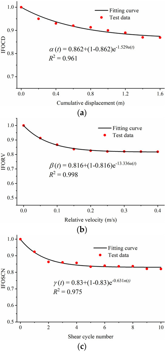
Figure 1.
The laboratory test results [27,32] and fitting curves with test data. (a) The variation law of IFOCD with cumulative displacement. (b) The variation law of IFORV with relative velocity. (c) The variation law of IFOSCN with shear cycle number.
As shown in Figure 1a, the influence factor of cumulative displacement α = 1 when the cumulative displacement u = 0. As the cumulative displacement increases, its influence factor gradually decreases, and then the decrease slows down, finally approaching a convergent value. As a whole, it is consistent with the form of the negative exponential function, and the IFORV and IFOSCN are similar to it. Therefore, the present study adopts Equation (4) to describe the variation of the influence factors.
where A, B, and C are the convergence values of the IFOCD, IFORV, and IFOSCN, respectively, and m, n, and p are the undetermined coefficients.
The fitting results are also shown in Figure 1. It can be seen from the figure that the fitting curve has high fitting accuracy on the test data points, and the coefficient of determination, R2, is above 0.96. It illustrates that it is reasonable to adopt Equation (4) to describe the variation law of each vibration deterioration influence factor of the structural plane. Parameters to be determined are as follows: A = 0.862, m = 1.529; B = 0.816, n = 13.336; C = 0.83, p = 0.631. After substituting the above parameters into Equations (3) and (4), the vibration deterioration factor of the structural plane at any time can be simplified as follows:
It should be noted here that the present study assumes that the deterioration factor will not increase with time after decreasing, so the deterioration factor in FDEM is set as monotonically decreasing.
2.3. Solution Steps of Dynamic Safety Factor Considering the Vibration Deterioration Effect
Xu et al. (2023) introduce the basic principle, solution steps, and simulation examples of the dynamic strength reduction method based on FDEM, demonstrating that the improved FDEM can analyze the dynamic stability of slopes under seismic load [4]. When it comes to research on landslides, the focus should be on the evolution process and formation mechanism of landslides. Therefore, considering that most earthquake-induced landslides are generated due to the gradual vibration deterioration of the structural plane, the present study proposes the dynamic strength reduction method based on the vibration deterioration of the structural plane, which can reproduce the formation and evolution mechanism of the earthquake-induced landslides as well as give a quantitative evaluation index of the dynamic safety with reference significance. The specific solution steps are as follows:
- (1)
- Establish the FDEM model and mark the elements at the structural plane.
- (2)
- Static calculation stage: the bottom and lateral boundaries are fixed in the normal direction. The ground stress equilibrium is completed when the model kinetic energy reaches the set convergence value.
- (3)
- Static stability analysis stage: the tensile strength, friction angle and cohesion of the model are reduced, and the reduction factor is the static strength reduction factor (SSRF). The static safety factor (SSF) is denoted as SSRF when the landslide occurs.
- (4)
- Dynamic calculation stage: the bottom and lateral boundaries are converted to viscous and free-field boundary conditions, respectively. The dynamic loads are input from the bottom of the model.
- (5)
- Dynamic stability analysis stage: Since the slope stability under dynamic load is weaker than that under static condition, the initial value of the dynamic strength reduction factor (DSRF) is slightly smaller than that of SSF. After DSRF is selected, seismic waves are applied to the model, and the joint and adjacent triangular elements at the structural plane update the values of friction angle and cohesion in real-time according to the cumulative displacement, the relative velocity and the shear cycle number to simulate the vibration deterioration effect of the structural plane.
- (6)
- DSRF is reduced sequentially, and Step (5) is repeated until the landslide is observed. The DSRF, at this point, is denoted as the dynamic safety factor (DSF).
3. Characterization of Anchor Cable in FDEM
Anchor cables are the main preventive measure in slope engineering. Figure 2 compares the reinforced slope (yellow area) and the unreinforced slope (red area) of Zipingpu Water Conservancy Project during the Wenchuan earthquake, highlighting the importance and reliability of anchor cables. There is little information about anchor cables in FDEM, and the present study tries to study them by referring to the characterization method of anchor bolt in FDEM.
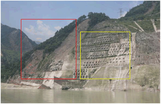
Figure 2.
Comparison of the reinforcement effect of the slope at the hole of sediment releasing tunnel of Zipingpu Water Conservancy Project.
3.1. The Existing Characterization of Anchor Bolts in FDEM
At present, there are two main methods for the characterization of anchor bolts in FDEM: one is the one-dimensional element model proposed by Zivaljic et al. (2013) [35] and Tatone et al. (2015) [36], which is mainly used for the simulation of steel bars in reinforced concrete structures and anchor bolts in tunnel engineering; the other is the entity element model proposed by Liu et al. (2019) [37] and Wang et al. (2022) [38] who both applied this method to rock bolt reinforcement in deep-buried tunnels.
- (a)
- One-dimensional element model
In the one-dimensional element model method, the bolt element is considered a one-dimensional, non-thickness line element. The coordinates of the two endpoints of each cable are given in the input file, and the intersections of the two endpoints with the triangular and joint elements are defined as reference points. The reference points are grouped in pairs to form calculation couples, where the calculation couple in the triangular element is called the bolt triangular element, and the one in the joint element is the bolt joint element (Figure 3).
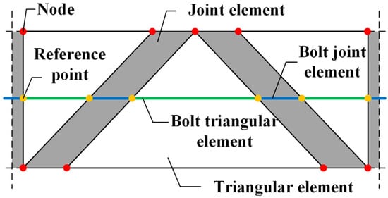
Figure 3.
Schematic of the one-dimensional bolt element [35].
The anchor bolt established by the one-dimensional element method has the following shortcomings:
- (1)
- The calculation process is cumbersome. Considering the complex stress path, the state of the anchor bolt needs to be determined in real-time, and the elastic foundation beam theory requires a large number of initial parameters and inadvertently increases programming costs, which is unfavorable to the calculation efficiency in large-scale numerical implementation.
- (2)
- Prestress cannot be applied. At present, prestressed cable bolt is widely used in many geotechnical projects, and the lack of this function dramatically limits the applicability of this technology.
- (3)
- The failure criterion of the bolt is doubtful. When a bolt joint element breaks, only this one fails and exits the calculation, while the other bolt triangular and bolt joint elements continue to play a role, which may make the analysis result too conservative.
- (4)
- The diameter of the bolt is ignored. At the laboratory test scale, the bolt occupies a specific space, which cannot be ignored relative to the sample size [34]. If the one-dimensional element method is adopted, it will inevitably intruduce errors in the calculation results.
- (5)
- The interaction and coupling mechanism between the cable and anchorage body, as well as between the rock mass and anchorage body, cannot be reflected. The calculation of the one-dimensional element method is carried out in the background and it applies the results to the corresponding node in the form of force. There is no entity element modeling such as anchor cable and anchor resin to participate in the calculation, and critical physical phenomena when various parts interact are missing.
- (b)
- Entity element model
The entity element model method focuses on studying the anchor bolt restraint mechanism and the interaction characteristics of the bolt structure with the anchorage body, which requires fine modeling of the anchor bolt and anchorage body [38]. Among them, the anchor bolt and anchorage body are divided into triangular and joint elements, as in the case of rock mass. The resin-bolt and resin-rock interfaces are characterized by the joint element (Figure 4). In specific engineering calculations, the physical and mechanical parameters of the anchor resin and bolt are the same as those of rock mass. They are calculated together until the anchor bolt comes into play. Then, the initial stress of the anchor resin and bolt is reset to zero, and their respective properties are assigned before recalculation [38]. As a metal material, anchor bolt has apparent yield and strain hardening phenomena, and its constitutive modification is required. More details about the constitutive model can be found in Liu et al. (2019) [37].
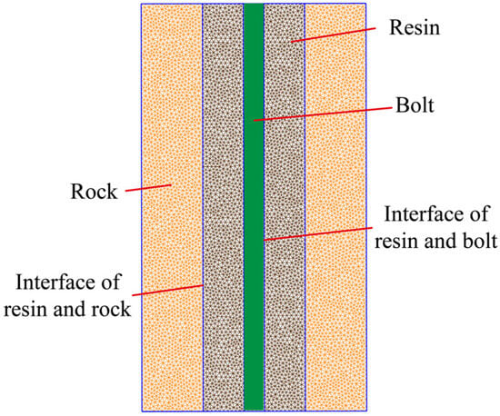
Figure 4.
Simplified bolt reinforced model [34].
As mentioned above, there are also shortcomings in the entity modeling method:
- (1)
- The modeling process is tedious. The coordinates and parameters of the anchor bolt and resin must be entered individually.
- (2)
- Local mesh subdivision at the anchor bolt and resin will result in a huge difference in size between the maximum and minimum mesh size, which will significantly increase the computational burden [37].
- (3)
- The process of prestressing is cumbersome. The model first performs the integral calculation, outputs the node coordinate data, and then substitutes them into the new input file for the secondary calculation. At the same time, the new input file needs to update the parameters of the anchor bolt and resin.
- (4)
- The method of prestressing is doubtful. During prestressing, tensile stress should be applied at the outer end of the anchor bolt, and compressive stress should be applied on the anchor plate to simulate the prestressing. However, it is doubtful whether the pressure on each part of the free segment of the anchor bolt can be transferred to the resin for the full-length bonded anchor bolt.
- (5)
- Predeformation of the anchor bolt: When the material adjacent to the bolt is deformed during the calculation stage where the bolt is not yet functioning, the geometry of the bolt will show non-negligible deformation, so it is not guaranteed that the bolt and resin remain straight in the subsequent stage of the calculation.
3.2. The Combined One-Dimensional and Entity Element Models in FDEM
The number of elements to divide a centimeter-scale anchor bolt model in a slope model with a height of hundreds of meters is huge (the diameter of the bolt has a limited effect on the calculation result of the whole model). At the same time, FDEM is an explicit algorithm, and small mesh sizes mean small time steps, which can lead to a geometric increase in the calculation time for a constant total physical time. In addition, many studies have demonstrated that the anchor cable failure generally occurs at the resin–rock interface or the anchor cable itself breaks (assuming that the free segment of the anchor cable can only bear the axial stress) [39]. Here, the cable, resin, and rock in the anchorage segment can be considered as a whole (i.e., anchorage body), so there is no need to consider the separate modeling of the anchor cable and resin, which can also be significant for studying the evolution law of the landslide–anchorage structure system while ensuring the accuracy and efficiency of the calculations. Therefore, entity modeling of the cable and resin is not desirable in the present study, but entity element modeling is still required to characterize the anchorage body. Finally, after describing the advantages and disadvantages of the anchor bolt characterization methods in the previous section, the combined one-dimensional and entity element model (ODEEM) method for anchor cables in FDEM (Figure 5) is proposed based with the actual needs of this study and is improved as follows:
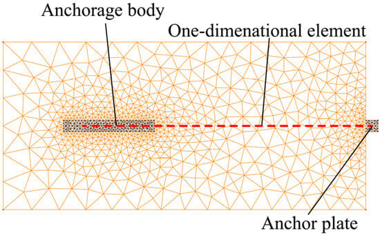
Figure 5.
Schematic of combined one-dimensional and entity element model (ODEEM) of anchor cable in FDEM.
- (1)
- Simplify the modeling process and optimize the mesh size distribution. During modeling, only the anchorage body and anchor plate need to be established, while the anchor cable in the free segment can be characterized by adding the coordinates of the two endpoints to the input file. As a result, the larger the geometry dimension of the anchorage body, the more uniform the mesh size of the entire model, and the fewer the total number of elements, which greatly improves the efficiency of the dynamics calculations and is beneficial to the application of FDEM at the engineering scale.
- (2)
- Realizing prestressing in one-dimensional element model method and simplifying the process. Prestress is pre-considered in the constitutive relation of the bolt triangular element, which can transfer the pre-compressive stress of each segment of the anchor cable to the corresponding rock. Furthermore, the application process is simple: just write the setting value of the prestress in the input file.
- (3)
- Optimize the calculation process by adding a simplified constitutive relation of the anchor cable. The constitutive relation of the bolt joint element in the one-dimensional element method is complicated, and the calculation efficiency is low. Moreover, the object of the present study is the anchor cable, which is assumed not to be subjected to shear stresses. Therefore, a simplified anchor cable constitutive relation is added, as detailed below.
FDEM divides the mesh into triangular elements and joint elements, where the triangular elements are only capable of linear elastic deformation, while the yielding and failure of the material are characterized by the joint elements. The bolt material in the one-dimensional element method is also applicable to the above principle, where the triangular elements are still subjected to linear deformation only, and the yielding, hardening, and failure phenomena of the bolt all occur in the joint elements. The ODEEM method refers to the bolt’s constitutive law proposed by Liu et al. (2019) [37] and is appropriately simplified based on the anchor cable, which is the object of study (Figure 6), as shown in Equation (6). It is assumed that the free segment of the anchor cable does not bear compression and bending moment, and only axial tensile stress. The axial tension has an obvious yielding phenomenon, and after reaching the yield limit εh, the material enters the hardening stage, which is assumed to be linear here with a hardening coefficient K (Equation (7)) [40], and the cyclic loading and unloading of the anchor cable is not considered.
where εb is the axial strain of the anchor cable in the joint element, εy is the axial yield strain, εh is the axial hardening strain, εu is the ultimate strain in the axial hardening stage (failure strain), σy is the axial yield stress, and σu is the axial ultimate stress (failure stress).
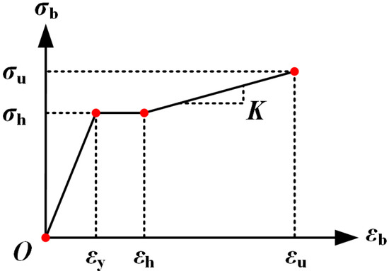
Figure 6.
The constitutive law of anchor cable in the joint element [33].
4. FDEM Simulation of the Entire Dynamic Evolution Process of the Landslide–Anchorage Structure System Under Earthquake
4.1. Computational Model
The landslide model of Baihua Bridge is generalized to obtain a rock slope containing a weak structural plane (Figure 7). To improve the slope stability, anchor cables are employed for reinforcement to prevent the potential landslide from sliding along the structural plane. The slope is divided into two steps, both with a slope angle of 53°. The cables are distributed along the slope surface with a spacing of 2.5 m and numbered from N0–N5 with lengths of 13 m, 12 m, 11 m, 10 m, 9 m, and 8 m. In Figure 7, P0–P24 are monitoring points, whose acceleration, velocity, and displacement are recorded during calculation. The physical and mechanical parameters of bedrock, potential sliding body, anchorage body, structural plane and anchor cable are shown in Table 1, Table 2 and Table 3. The local damping coefficient of the model is 0.125.
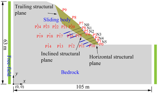
Figure 7.
FDEM model of the landslide–anchorage structure system.

Table 1.
Physical and mechanical parameters of the bedrock and sliding body.
Table 2.
Physical and mechanical parameters of the structural plane and the interface of the anchorage body and rock mass.
Table 3.
Physical and mechanical parameters of the anchor cable.
In order to study the dynamic evolution of the landslide–anchorage structural system under seismic load, eight computational models with four different seismic intensities (VII, VIII, IX, and X) are established for the two calculation conditions: anchor cable-unreinforced and -reinforced, respectively.
4.2. Results
4.2.1. Dynamic Response Analysis of the Landslide–Anchorage Structure System
Taking the landslide–anchorage structural system as a whole, the dynamic response characterization can reveal its failure process and mechanism, and ultimately provide theoretical basis and data support for the analysis of the entire dynamic evolution process.
The PGA amplification factor is the ratio of the maximum acceleration at any point on the slope to the maximum acceleration at P0. Acceleration response analysis is mainly used in the finite element method [20] and in the discrete cell method, especially when applied in the FDEM, which can simulate the entire dynamic evolution process of the landslide. It is first necessary to determine the time point when an obvious collision between the blocks occurs during the sliding process, because when the sliding body undergoes an overall failure, the gravitational acceleration and the contact force caused by collision will affect the acceleration value at the monitoring point. Moreover, the conversion of static–dynamic boundary conditions is involved in the present paper, and it can lead to small fluctuations in acceleration during this process [23]. Therefore, the time history of acceleration at monitoring points in this section ranges from 0.1 s after the static–dynamic transition to the collision of sliding blocks. The variation of PGA amplification factor along different measurement lines (P0–P9 along the slope surface, P0–P14, P19–P4, P24–P7 in the horizontal direction) under different seismic intensities is shown in Figure 8.
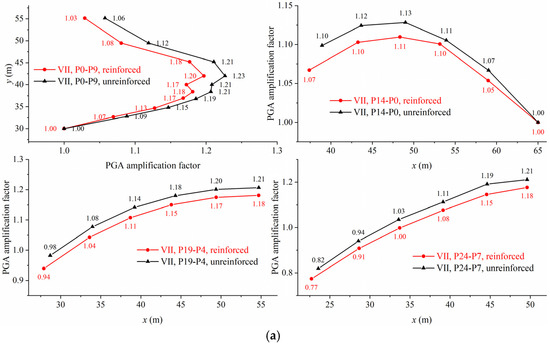
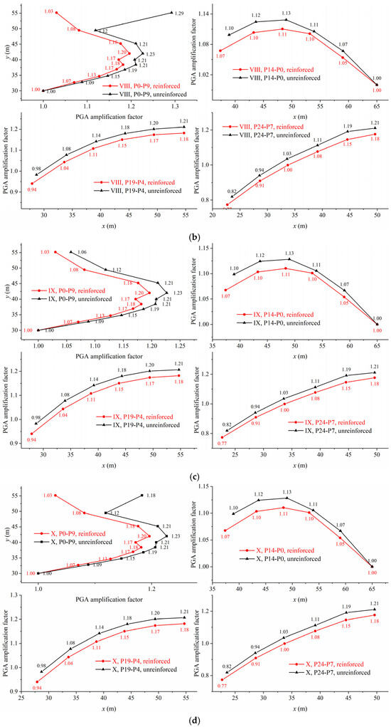
Figure 8.
Comparison of variations in the PGA amplification factors for the unreinforced and cable-reinforced slopes. (a) Seismic intensity VII (1.1 s–11 s). (b) Seismic intensity VIII (1.1 s–9.66 s). (c) Seismic intensity IX (1.1 s–7.2 s). (d) Seismic intensity X (1.1 s–6.2 s).
The dynamic response of the unreinforced slope and the cable-reinforced slope is inconsistent under dynamic load. Still, on the whole, the dynamic response of the cable-reinforced slope is weaker than that of the unreinforced slope. Taking seismic intensity VIII as an example, the PGA amplification factor at the slope surface can be lower by 4% on average, about 1.4% at P14–P0 in the horizontal direction, 3% at P19–P4, and 3.8% at P24–P7. This is attributed to the ability of prestressed anchor cables to strengthen the slope and form a more rigid whole with it, which can significantly reduce the PGA of the slope under dynamic load. As shown in Figure 9, the acceleration time history at P9 at the top of the slope also confirms this because the existence of a prestressed anchor cable, on one hand, improves the integrity and joint strength of the slope, and on the other hand, reduces the vibration acceleration of the slope.
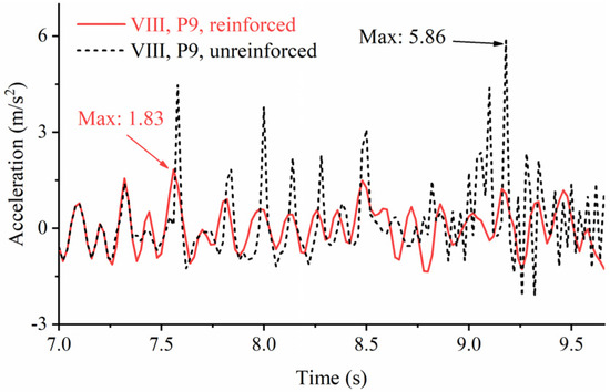
Figure 9.
The acceleration time history of monitoring point P9 of the unreinforced and cable-reinforced slopes at seismic intensity VIII.
Moreover, it is also found that the PGA amplification factors of the unreinforced and cable-reinforced slopes at the slope surface are significantly larger than those inside the slope, which is due to the wave superposition effect that occurs as a result of the stress wave transfer to the free face. For both unreinforced and cable-reinforced slopes, there is a significant elevation amplification effect from the slope toe to 0.5 times the slope height, with the PGA amplification factor increases along the slope surface with the rise in elevation. However, from 0.5 times the slope height to the top of the slope, the PGA amplification factor decreases. The reasons for the above are multifaceted and complex: the structural plane and the newly generated fracture surface have the effect of attenuating the stress wave, but the free face formed by them will have the effect of amplifying the stress wave. These two effects of attenuation and enhancement compete with each other within the slope, and this is the cause for the decrease in the PGA amplification factor with the elevation at the macro level.
In Figure 8, the variation of the PGA amplification factor with x coordinate at different elevations can be observed. It can be found that the application of anchor cables does not change the distribution trend of the PGA amplification factor inside the slope. The PGA amplification factor of the middle and top slopes has an evident tendency to have a horizontal surface effect, which increases with the decrease in the distance from the slope surface. The PGA amplification factor for the bottom slope is more complicated because the stress wave attenuates at the structural plane.
4.2.2. Analysis of Dynamic Evolution of the Anchor Cable Axial Force
Figure 10 shows the distribution of anchor cable axial force at t = 7 s under different seismic intensities. As the seismic intensity increases, the anchor cable axial force increases gradually. The strong dynamic load will intensify the magnitude of the slope movement, and the anchor cable can improve the integrity of the rock mass and connect the slope tightly, so it needs a larger axial force to resist the stripping effect of the seismic wave. A high value (437.12 kN, 437.05 kN, 436.07 kN and 409.764 kN) is observed in the anchor cable N0 near the slope surface at all seismic intensities, which is caused by the uncoordinated movement of the slope, and it can be inferred that fracture has occurred here by combining with the elevation amplification effect described above. Based on the distribution characteristics of the anchor cable axial force, the fracture of the slope body can be preliminarily judged. The structural plane is the weakest part of the slope, and the anchor cable axial force here increases the fastest with the variation of seismic intensity, which is higher than the other parts of the anchor cable at seismic intensity IX. This is more obvious at seismic intensity X because the structural plane fails, and the penetration plane and the sliding body are formed, so the anchor cable needs to increase its axial force to resist the dual effects of dynamic load and gravity. When the structural plane does not fail, taking seismic intensity VIII as an example, the axial forces of anchor cables N0–N5 at the structural plane are 5.249 kN, 4.618 kN, 4.57 kN, 3.384 kN, 2.857 kN, and 2.099 kN and show a decreasing trend because the distribution of PGA amplification factor within the slope follows the elevation amplification and horizontal surface effects, and the PGA amplification factor is correlated with the anchor cable axial force. When the structural surface fails, taking the seismic intensity IX as an example, the axial forces of the anchor cables N0–N5 at the structural plane are 75.008 kN, 66.945 kN, 73.612 kN, 78.632 kN, 93.878 kN, and 127.694 kN. The anchor cables N0–N2 of the second step have no apparent law, and the effect of seismic waves plays a dominant role here. The anchor cables N3–N5 of the first step show an increasing trend and are larger than the anchor cables of the second step because here they are greatly affected by gravity, and the larger the volume of the sliding body, the greater the effect of gravity.
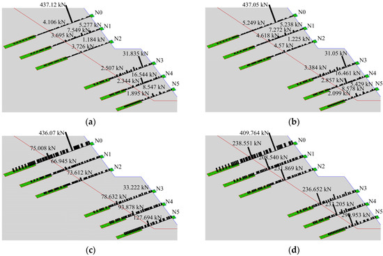
Figure 10.
The diagrams of anchor cable axial force at t = 7 s for all seismic intensities. (a) Seismic intensity VII. (b) Seismic intensity VIII. (c) Seismic intensity IX. (d) Seismic intensity X.
Figure 11 is the time history of the anchor cable axial force at the structural plane under different seismic intensities. It can be seen from the figure that with the increase in seismic intensity, the axial force of each anchor cable grows larger to a different degree (the average maximum axial force of anchor cables under each seismic intensity: VII is 161.165 kN, VIII is 364.878 kN, IX is 563.883 kN, and X ≥ 648 kN). The growth rate is related to the cable location and the seismic waveform (take VII for example, the mutation of the axial force in Figure 11a corresponds to the local peak of the seismic wave), the lowest anchor cable N5 grows the fastest, while cables N4–N0 slow down roughly in order. At the end of the earthquake, the maximum anchor cable axial force does not seem to conform to the law of decreasing from bottom to top, which is related to the seismic waveform and the physical and mechanical properties of the slope; the generation order of crack and the distribution of the stress wave will affect the stress state of the anchor cable, and eventually present an irregular maximum axial force. Anchor cable first fails in the hazardous area and then gradually spreads, and its failure sequence is also related to the seismic wave characteristics. When the seismic intensity is X, the failure sequence of the anchor cable is N0 (10.06 s)-N2 (10.09 s)-N1 (10.32 s)-N3 (10.36 s)-N4 (10.48 s)-N5 (10.6 s), which exhibits noticeable continuous failure effect and is consistent with the distribution of PGA amplification factors in Figure 8d. Therefore, the continuous failure effect of anchor cables should be considered in the anchorage system design process, but the present study does not continue to investigate it in depth, and the authors will continue to carry out the research related to anchor cables in FDEM in future work.
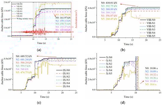
Figure 11.
Time histories of anchor cable axial force at the structural plane under different seismic intensities. (a) Seismic intensity VII. (b) Seismic intensity VIII. (c) Seismic intensity IX. (d) Seismic intensity X.
4.2.3. Analysis of Entire Dynamic Evolution Process of the Landslide–Anchorage Structure System
Figure 12 is the schematic diagram of the entire process of landslide dynamic evolution under unreinforced conditions at different seismic intensities. From the figure, it can be seen that the evolution process under different seismic intensities has commonalities and can be roughly divided into the following stages:
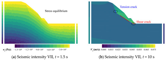
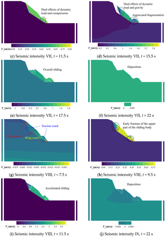
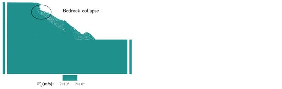
Figure 12.
Schematic diagram of the entire process of landslide dynamic evolution under unreinforced condition at different seismic intensities (similar process is omitted).
- (1)
- Initial ground stress equilibrium stage (Figure 12a). This stage takes 1.5 s. The kinetic energy of the model is calculated to be within 50 J, and then the dynamic calculation stage begins. The static boundary conditions are converted into dynamic boundary conditions, and the seismic loads are loaded at the bottom of the main model and the free field at the same time.
- (2)
- Sliding surface penetration stage. When the seismic intensity is VII, tensile cracks caused by reciprocating dynamic loads first appear at the toe of the lower part of the inclined sliding surface at t = 10 s (7.27 s for VIII, 6.33 s for IX, and 5.45 s for X), followed by shear failures on the horizontal sliding surface, and tensile failures on the lower part of the trailing edge structural plane (Figure 12b); and finally, t = 10.02 s (7.5 s for VIII, 6.45 s for IX, and 5.48 s for X), the inclined sliding surface and the trailing edge structural surface keep extending to penetration for shear failures under the dual effects of gravity and seismic load (Figure 12g). At this stage, the crack number of the model at all seismic intensities grows to 98 (Figure 13), and the time required for the sliding surface to penetrate continues to decrease with increasing seismic intensity. As shown in Figure 14, the model kinetic energy changes little in this stage and is caused only by seismic loads.
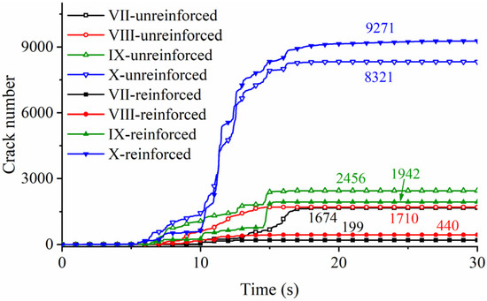 Figure 13. Variation of crack number of the model under different calculation conditions.
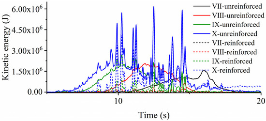 Figure 14. Variation of kinetic energy of the model under different calculation conditions.
 - (3)
- Dynamic failure stage. When the seismic intensity is VII, t = 11.5 s, under the dual effects of dynamic load and sliding extrusion, the rock mass at the lower part of the sliding body is gradually fragmented (Figure 12c), and the crack number grows to 246 (Figure 13), and the kinetic energy of the model starts to increase dramatically at this point (Figure 14). After the sliding body slides down for a certain distance as a whole, the block at the upper free face is gradually ruptured, and the block starts to spall and fall (Figure 12d, t = 15.5 s), the crack number surges to 830 (Figure 13), the falling blocks collide with the slope surface resulting in the intensification of the degree of fragmentation (Figure 12e, t = 17.5 s), and the crack number becomes 1638. The kinetic energy also reaches the maximum value during this stage (Figure 14, 1,537,878 J, t = 15.97 s). Other seismic intensities show some different characteristics at this stage: at seismic intensity VIII, the rock mass at the upper of the sliding body is fractured before the sliding body slides down (Figure 12h, t = 9.5 s), and the landslide occurs at t = 11.5 s (Figure 12i). The maximum crack number and kinetic energy at this stage also become larger with the increase in seismic intensity, which is 1313 (Figure 13, t = 12.48 s) and 2,086,209 J (Figure 14, t = 12.48 s), respectively; the evolution process at seismic intensities IX and X is the same as that at intensity VIII, in which the maximum crack number and kinetic energy increase with the seismic intensity (IX: 1456, 2,679,335 J, t = 10.24 s; X: 1547, 5,725,569 J, t = 10.23 s). However, due to the increase in seismic intensity, the bedrock also fractures at intensity IX (Figure 12j), and even partially collapses at intensity X (Figure 12k).
- (4)
- Energy dissipation stage. When the seismic intensity is VII, the kinetic energy of the model starts to decrease after 15.97 s under the effect of the energy dissipation mechanism, during which the sliding body is squeezed and collides while moving, and the crack number further increases in a small amount and reaches the maximum value of 1647 at 18.2 s (Figure 13). The model finally stops moving at the end of the earthquake (t = 22 s) (Figure 12f). At the seismic intensities VIII and IX, the kinetic energy of the model starts to decrease at 12.48 s and 12.24 s, and the maximum values of the crack number are 1709 (Figure 13, 15.8 s) and 2456 (Figure 13, 16.5 s), respectively. When the seismic intensity is X, the kinetic energy of the model starts to decrease at 12.48 s, but due to the high intensity of the earthquake, the upper bedrock also collapses and is destroyed, and the kinetic energy peaks several times and reaches 0 at 22 s (Figure 14); the final crack number is 8321 (Figure 13, 19.36 s).
The schematic diagram of the dynamic evolution of the landslide–anchorage structure system at all seismic intensities is shown in Figure 15. Among them, when the seismic intensities are VII, VIII, and IX, the anchor cables are intact and no landslide occurs; when the seismic intensity is X, the anchor cables fail in order, and overall failure occurs in the landslide–anchorage structural system. The above dynamic evolution process can be roughly divided into the following stages:
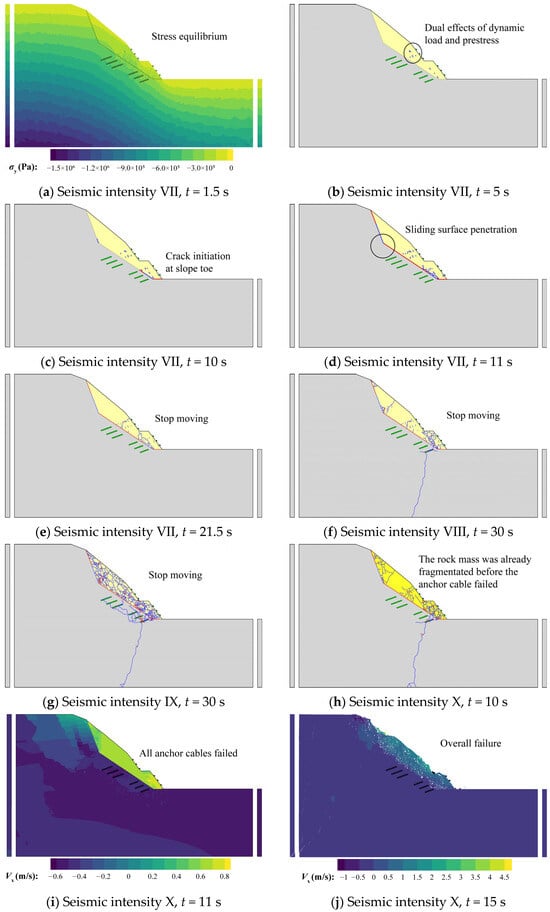
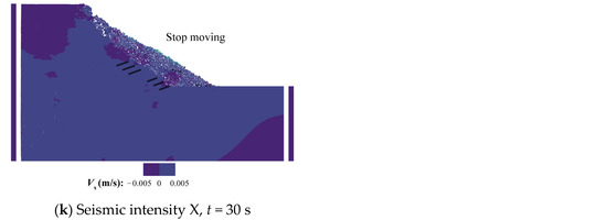
Figure 15.
Schematic diagram of the entire dynamic evolution process of the landslide–anchorage structure system at different seismic intensities (similar process is omitted).
- (1)
- Initial ground stress equilibrium stage (Figure 15a).
- (2)
- Rock mass near the free segment of the anchor cable failure stage. Prestresses are generated in the rock mass in the vicinity of the anchor cables after the anchor cables are prestressed, and with the application of seismic loads, the stress concentration enables this part of the rock mass to be more prone to fracture (Figure 15b, t = 5 s). This stage is observed at all seismic intensities.
- (3)
- Sliding surface penetration stage. This stage is the same as the dynamic evolution law of the unreinforced condition: take seismic intensity VII as an example, the toe of the inclined sliding surface is the first to tensile failure caused by the reciprocating motion of the dynamic load at t = 9.98 s; then, shear failure occurs almost simultaneously at the horizontal structural plane, tensile failure occurs at the lower part of the trailing edge of the structural plane (Figure 15c, t = 10 s), and finally, the inclined sliding surface and the trailing edge of the structural plane continue to extend to penetration under the dual effects of gravity and seismic load at t = 11 s (Figure 15d). For other seismic intensities (Figure 16), the crack initiation time is 7.26 s for VIII, 6.24 s for IX, and 5.46 s for X, and the sliding surface penetration time is 9.31 s for VIII, 7.02 s for IX, and 5.91 s for X. It can be seen that the crack initiation time and penetration time of the structural plane are advanced with the increase in the seismic intensity. At the time of structural plane penetration, the crack number of the model at each seismic intensity is 129 (VII), 130 (VIII), 151 (IX), and 141 (X), showing an overall increasing trend and indicating that the number of secondary cracks at this stage is positively correlated with the seismic intensity. The kinetic energies of the model at the end of this stage are 9240 J (VII), 12,073 J (VIII), 21,837 J (IX) and 27,148 J (X), which is mainly related to the input seismic wave energy. The landslide–anchorage structural system does not fail under seismic intensities VII, VIII, and IX, and does not enter the overall damage stage after this stage; instead, it is further fragmented under seismic loads, but the landslide–anchorage structural system is still tightly integrated owing to the prestressed anchor cables (Figure 15f,g). The final crack numbers are 199, 440, and 1492 for intensities VII, VIII, and IX, respectively (Figure 13), and the law is apparent: the damage degree of the landslide–anchorage structure system increases with the increase in seismic intensity.
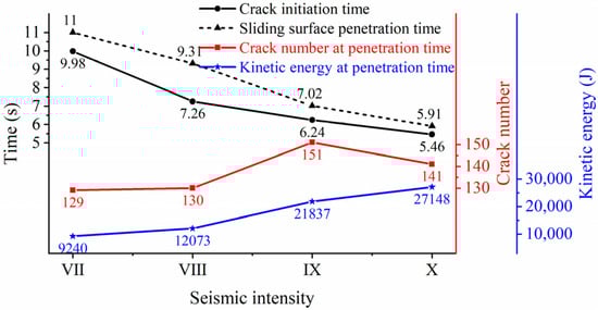 Figure 16. Comparison of crack initiation and penetration time, and crack number and kinetic energy at penetration time under different seismic intensities.
 - (4)
- Overall failure stage. The landslide–anchorage structure system occurs overall failure under seismic intensity X. It can be seen from Figure 11d that the anchor cable N0 at the toe of the slope fails first at t = 10.06 s, followed by anchor cable N2 at t = 10.08 s and N1 at t = 10.32 s, and the failure sequence is consistent with the distribution of PGA amplification factor in Figure 8d. After the second step anchor cables N0–N2 failure, the first step anchor cables N3–N5 fail sequentially under the dual effects of gravity and seismic load (t = 10.36 s, t = 10.48 s, t = 10.6 s). Before the anchor cable N0 fails, as shown in Figure 15h, the slope becomes fragmented, and the crack number is 655, which is much smaller than the crack number of 1431 in the unreinforced slope at the same time, indicating that the prestressed anchor cable can connect the slope and the anchorage system as a whole, thus significantly reducing the probability of landslides. When all anchor cables fail at t = 11 s, overall failure occurs in the landslide–anchorage structure system (Figure 15i,j).
- (5)
5. Conclusions
In the present study, the algorithm of FDEM is improved in depth: the vibration deterioration model of structural plane is added, the solution steps of the dynamic safety factor considering the vibration deterioration effect of structural plane are provided; by comparing and analyzing the existing bolt element model in FDEM, the combined one-dimensional and entity element model of anchor cable element is proposed, and the generalization model for the landslide–anchorage structure system during earthquake is established to discuss the dynamic response law and entire evolution process of the landslide–anchorage structural system. The main conclusions are as follows:
- (a)
- Considering that the most significant inducement factor of earthquake-induced rock landslides is the gradual vibration deterioration on the structural plane, the present study proposes a dynamic strength reduction method for FDEM, which considers the effects of cumulative displacement, relative velocity, and shear cycle number. Based on this method, the entire damage process of earthquake-induced landslide can be reproduced, and its internal evolution mechanism can be deeply investigated; in addition, this method can give a quantitative evaluation index of dynamic safety with practical significance, and it can be promoted and applied in the field of seismic design of slopes.
- (b)
- The advantages of the combined one-dimensional and entity element model of the anchor cable in FDEM are as follows: (1) simplifying the modeling process and optimizing the mesh size distribution; (2) realizing the prestress application by the one-dimensional element model and simplifying the application process; and (3) optimizing the calculation process by simplifying the constitutive law of anchor cable.
- (c)
- Based on the generalized slope model, the entire process of dynamic evolution of landslide–anchorage structure system under seismic load is investigated: (1) the dynamic response of unreinforced and cable-reinforced slopes is inconsistent, but overall, the dynamic response of the cable-reinforced slope is obviously smaller than that of the unreinforced slope, which is due to the fact that the presence of prestressed anchor cable improves the integrity of slope body and the strength of joints on the one hand, while on the other hand, it reduces the slope’s vibration acceleration; (2) the distribution of PGA amplification factor within the slope is nonlinear, and the reason for this is multifaceted and complex; the structural plane and the newly generated fracture surface have the effect of attenuating the stress wave, but the free face formed by them will have the effect of amplifying the stress wave. These two effects of attenuation and enhancement compete with each other within the slope, and the results show nonlinear characteristics in the macro sense; (3) with the increase in seismic intensity, the axial force of the anchor cable also increases gradually; (4) the axial force at the structural plane and fracture surface is larger, and the PGA amplification factor has a correlation with the axial force of the anchor cable; therefore, according to the distribution characteristics of the axial force and the PGA amplification factor, the fracture of the slope can be preliminarily judged; (5) the crack initiation and penetration times advance with the increase in the seismic intensity, and the crack number and kinetic energy at the penetration time increase with the increase in the seismic intensity.
Author Contributions
Methodology, Validation, Formal analysis, and Writing, C.X.; Conceptualization, Supervision, and Funding acquisition, Y.H.; Writing, Review and Editing, G.L.; Software, C.M.; Investigation, M.L. All authors have read and agreed to the published version of the manuscript.
Funding
This research was funded by the Basic Research Fund for Central Public Research Institutes (CKSF20241007/YT) and the National Natural Science Foundation of China (52279093).
Institutional Review Board Statement
Not applicable.
Informed Consent Statement
Not applicable.
Data Availability Statement
The data presented in this study are available upon request from the corresponding author.
Acknowledgments
The work of this paper is based on Y2D of Munjiza et al. and Y-Geo and Y-GUI of Grasselli’s Geomechanics Group (http://www.geogroup.utoronto.ca/) (accessed on 15 August 2019).
Conflicts of Interest
The authors declare no conflicts of interest.
References
- Zhang, Y. Multi-field Characteristics and Evolution Mechanism of Majiagou Landslide-Stabilizing Piles System under Reservoir Operations. Master’s Thesis, China University of Geosciences, Wuhan, China, 2018. [Google Scholar]
- Yin, X.; Cheng, S.; Yu, H.; Pan, Y.; Liu, Q.; Huang, X.; Gao, F.; Jing, G. Probabilistic assessment of rockburst risk in TBM-excavated tunnels with multi-source data fusion. Tunn. Undergr. Space Technol. 2024, 152, 105915. [Google Scholar] [CrossRef]
- Iverson, R.M. Landslide triggering by rain infiltration. Water Resour. Res. 2000, 36, 1897–1910. [Google Scholar] [CrossRef]
- Xu, C.; Liu, Q.; Tang, X.; Sun, L.; Deng, P.; Liu, H. Dynamic stability analysis of jointed rock slopes using the combined finite-discrete element method (FDEM). Comput. Geotech. 2023, 160, 105556. [Google Scholar] [CrossRef]
- Ng, C.W.W.; Zhan, L.; Bao, C.G.; Fredlund, D.D.; Gong, B.W. Performance of an unsaturated expansive soil slope subjected to artificial rainfall infiltration. Géotechnique 2003, 2, 143–157. [Google Scholar] [CrossRef]
- Tu, X.B.; Kwong, A.K.L.; Dai, F.C.; Tham, L.G.; Min, H. Field monitoring of rainfall infiltration in a loess slope and analysis of failure mechanism of rainfall-induced landslides. Eng. Geol. 2009, 105, 134–150. [Google Scholar] [CrossRef]
- Rodríguez, C.E.; Bommer, J.J.; Chandler, R.J. Earthquake-induced landslides: 1980–1997. Soil Dyn. Earthq. Eng. 1999, 18, 325–346. [Google Scholar] [CrossRef]
- Keefer, D.K. Statistical analysis of an earthquake-induced landslide distribution—the 1989 Loma Prieta, California event. Eng. Geol. 2000, 58, 231–249. [Google Scholar] [CrossRef]
- Bhandari, T.; Hamad, F.; Moormann, C.; Sharma, K.G.; Westrich, B. Numerical modelling of seismic slope failure using MPM. Comput. Geotech. 2016, 75, 126–134. [Google Scholar] [CrossRef]
- Peng, Y.; Dong, S.; Lu, Z.; Zhang, H.; Hou, W. A method for calculating permanent displacement of seismic-induced bedding rock landslide considering the deterioration of the structural plane. Front. Earth Sci. 2023, 10, 1026310. [Google Scholar] [CrossRef]
- Wu, H.; Wu, Z.; Lei, H.; Lai, T. Application of BRFP New-Type Anchor Cable Material in High Slopes against Earthquakes. Adv. Civ. Eng. 2021, 2021, 1–19. [Google Scholar] [CrossRef]
- Zhang, J.J.; Niu, J.Y.; Fu, X.; Cao, L.C.; Yan, S.J. Failure modes of slope stabilized by frame beam with prestressed anchors. Eur. J. Environ. Civ. Eng. 2022, 26, 2120–2142. [Google Scholar] [CrossRef]
- Yin, X.; Liu, Q.; Lei, J.; Pan, Y.; Huang, X.; Lei, Y. Hybrid deep learning-based identification of microseismic events in TBM tunnelling. Measurement 2024, 238, 115381. [Google Scholar] [CrossRef]
- Wu, Q.; Liu, Y.; Tang, H.; Kang, J.; Wang, L.; Li, C.; Wang, D.; Liu, Z. Experimental study of the influence of wetting and drying cycles on the strength of intact rock samples from a red stratum in the Three Gorges Reservoir area. Eng. Geol. 2023, 314, 107013. [Google Scholar] [CrossRef]
- Zheng, Y.; Wang, R.; Chen, C.; Sun, C.; Ren, Z.; Zhang, W. Dynamic analysis of anti-dip bedding rock slopes reinforced by pre-stressed cables using discrete element method. Eng. Anal. Bound. Elem. 2021, 130, 79–93. [Google Scholar] [CrossRef]
- Wang, J.; Wang, S.; Su, A.; Xiang, W.; Xiong, C.; Blum, P. Simulating landslide-induced tsunamis in the Yangtze River at the Three Gorges in China. Acta Geotech. 2021, 16, 2487–2503. [Google Scholar] [CrossRef]
- Sun, L.; Liu, Q.; Abdelaziz, A.; Tang, X.; Grasselli, G. Simulating the entire progressive failure process of rock slopes using the combined finite-discrete element method. Comput. Geotech. 2022, 141, 104557. [Google Scholar] [CrossRef]
- Peng, N.; Dong, Y.; Zhu, Y.; Hong, J. Influence of Ground Motion Parameters on the Seismic Response of an Anchored Rock Slope. Adv. Civ. Eng. 2020, 2020, 1–10. [Google Scholar] [CrossRef]
- Stead, D.; Eberhardt, E.; Coggan, J.S. Developments in the characterization of complex rock slope deformation and failure using numerical modelling techniques. Eng. Geol. 2006, 83, 217–235. [Google Scholar] [CrossRef]
- Jia, Z.; Tao, L.; Bian, J.; Wen, H.; Wang, Z.; Shi, C.; Zhang, H. Research on influence of anchor cable failure on slope dynamic response. Soil Dyn. Earthq. Eng. 2022, 161, 107435. [Google Scholar] [CrossRef]
- Li, L.; Ju, N.; Zhang, S.; Deng, X.; Sheng, D. Seismic wave propagation characteristic and its effects on the failure of steep jointed anti-dip rock slope. Landslides 2019, 16, 105–123. [Google Scholar] [CrossRef]
- Xu, C.; Liu, Q.; Wu, J.; Deng, P.; Liu, P.; Zhang, H. Numerical study on P-wave propagation across the jointed rock masses by the combined finite-discrete element method. Comput. Geotech. 2022, 142, 104554. [Google Scholar] [CrossRef]
- Xu, C.; Liu, Q.; Xie, W.; Wang, Y.; Li, S.; Lu, W.; Zhang, H. Investigation on artificial boundary problem in the combined finite-discrete element method (FDEM). Comput. Geotech. 2022, 151, 104969. [Google Scholar] [CrossRef]
- Ye, Z.; Xie, J.; Lu, R.; Wei, W.; Jiang, Q. Simulation of Seismic Dynamic Response and Post-failure Behavior of Jointed Rock Slope Using Explicit Numerical Manifold Method. Rock Mech. Rock Eng. 2022, 55, 6921–6938. [Google Scholar] [CrossRef]
- Munjiza, A. The Combined Finite-Discrete Element Method; Wiley: West Sussex, UK; Hoboken, NJ, USA; London, UK, 2004. [Google Scholar]
- Munjiza, A.; Bangash, T.; John, N.W.M. The combined finite–discrete element method for structural failure and collapse. Eng. Fract. Mech. 2004, 71, 469–483. [Google Scholar] [CrossRef]
- Wang, S.; Zhang, J. On the dynamic stability of block sliding on rock slopes. Sci. Geol. Sin. 1982, 02, 162–170. [Google Scholar]
- Qi, S. Evaluation of the permanent displacement of rock mass slope considering deterioration of slide surface during earthquake. Chin. J. Geotech. Eng. 2007, 29, 452–457. [Google Scholar]
- Newmark, N.M. Effect of earthquake on dams and embankments. Géotechnique 1965, 15, 139–159. [Google Scholar] [CrossRef]
- Liao, S. Study on Stability of Block Rock Slope Under Strong Earthquake. Ph.D. Thesis, China University of Geosciences, Wuhan, China, 2013. [Google Scholar]
- Lee, H.S.; Park, Y.J.; Cho, T.F.; You, K.H. Influence of asperity degradation on the mechanical behavior of rough rock joints under cyclic shear loading. Int. J. Rock Mech. Min. Sci. 2001, 38, 967–980. [Google Scholar] [CrossRef]
- Ni, W. Time-Varying Stability Analysis of Slope Based on Dynamic Deterioration of Geomaterials. Ph.D. Thesis, China University of Geo-sciences, Wuhan, China, 2014. [Google Scholar]
- Ni, W.; Tang, H.; Liu, X.; Wu, Y. Dynamic stability analysis of rock slope considering vibration deterioration of struc-tur-al planes under seismic loading. Chin. J. Rock Mech. Eng. 2013, 32, 492–500. [Google Scholar]
- Wang, G.; Zhang, C.; Peng, G.; Chen, C. Dynamic test of rigid blocks and parameter study in dynamic analysis of distinct elements. Chin. J. Rock Mech. Eng. 1994, 02, 124–133. [Google Scholar]
- Zivaljic, N.; Smoljanovic, H.; Nikolic, Z. A combined finite-discrete element model for RC structures under dynamic loading. Eng. Comput. 2013, 30, 982–1010. [Google Scholar] [CrossRef]
- Tatone, B.; Lisjak, A.; Mahabadi, O.; Vlachopoulos, N. Verification of the Implementation of Rock-Reinforcement Elements in Numerical Analyses Based on the Hybrid Combined Finite-discrete Element Method (FDEM). In Proceedings of the 49th US Rock Mechanics/Geomechanics Symposium, San Francisco, CA, USA, 29 June–1 July 2015. [Google Scholar]
- Liu, Q.; Deng, P.; Bi, C.; Li, W.; Liu, J. FDEM numerical simulation of the fracture and extraction process of soft sur-rounding rock mass and its rockbolt-shotcrete-grouting reinforcement methods in deep tunnel. Rock Soil Mech. 2019, 40, 4065–4083. [Google Scholar]
- Wang, W.; Ding, Z.; Ma, H.; Sun, W.; Ren, J. Simulation analysis on bolting and grouting reinforcement of fractured rock using GPU parallel FDEM. Geomech. Geophys. Geo-Energy Geo-Resour. 2022, 8, 175. [Google Scholar] [CrossRef]
- Long, Z. Shear Effects on the Anchorage Interfaces of a Rock Slope Containing a Weak Layer Under Seismic Action. Ph.D. Thesis, Lanzhou University, Lanzhou, China, 2020. [Google Scholar]
- Sun, D.; Lin, J.; Liu, R.; Hu, Q. Research on strength coefficient in power hardening model of sheet metal. J. Plast. Eng. 2009, 16, 149–152. [Google Scholar]
Disclaimer/Publisher’s Note: The statements, opinions and data contained in all publications are solely those of the individual author(s) and contributor(s) and not of MDPI and/or the editor(s). MDPI and/or the editor(s) disclaim responsibility for any injury to people or property resulting from any ideas, methods, instructions or products referred to in the content. |
© 2025 by the authors. Licensee MDPI, Basel, Switzerland. This article is an open access article distributed under the terms and conditions of the Creative Commons Attribution (CC BY) license (https://creativecommons.org/licenses/by/4.0/).