
Unsupervised Feature Selection via a Dual-Graph Autoencoder with


Abstract
Featured Application
Abstract
1. Introduction
2. Related Work and Methods
2.1. Autoencoder
2.2. Dual-Graph Regularization
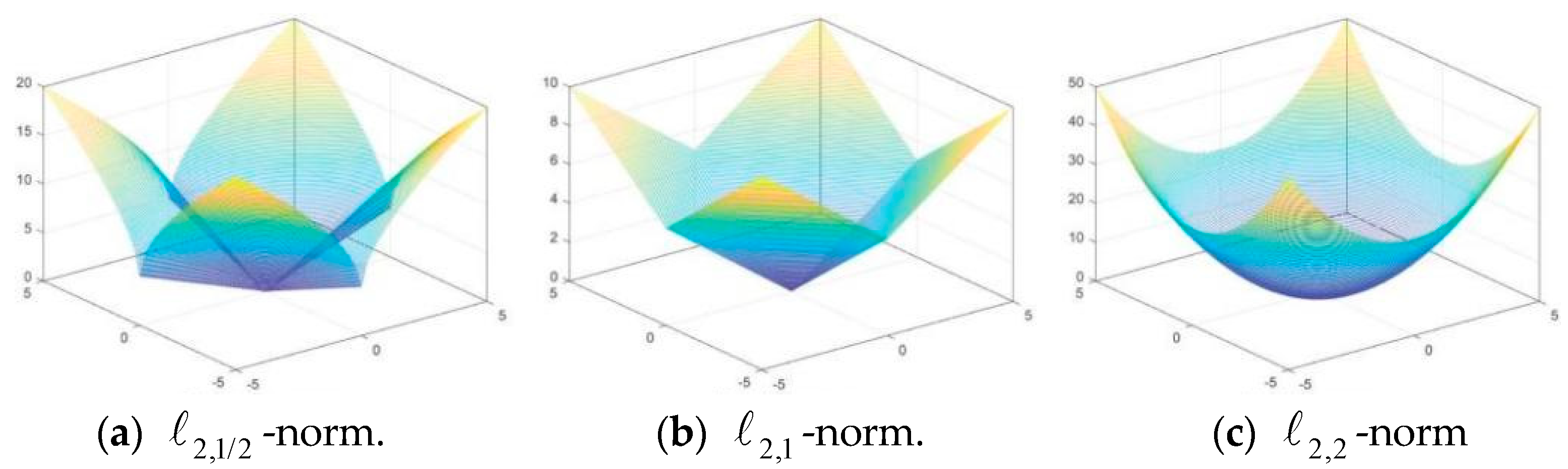
2.3. Norm
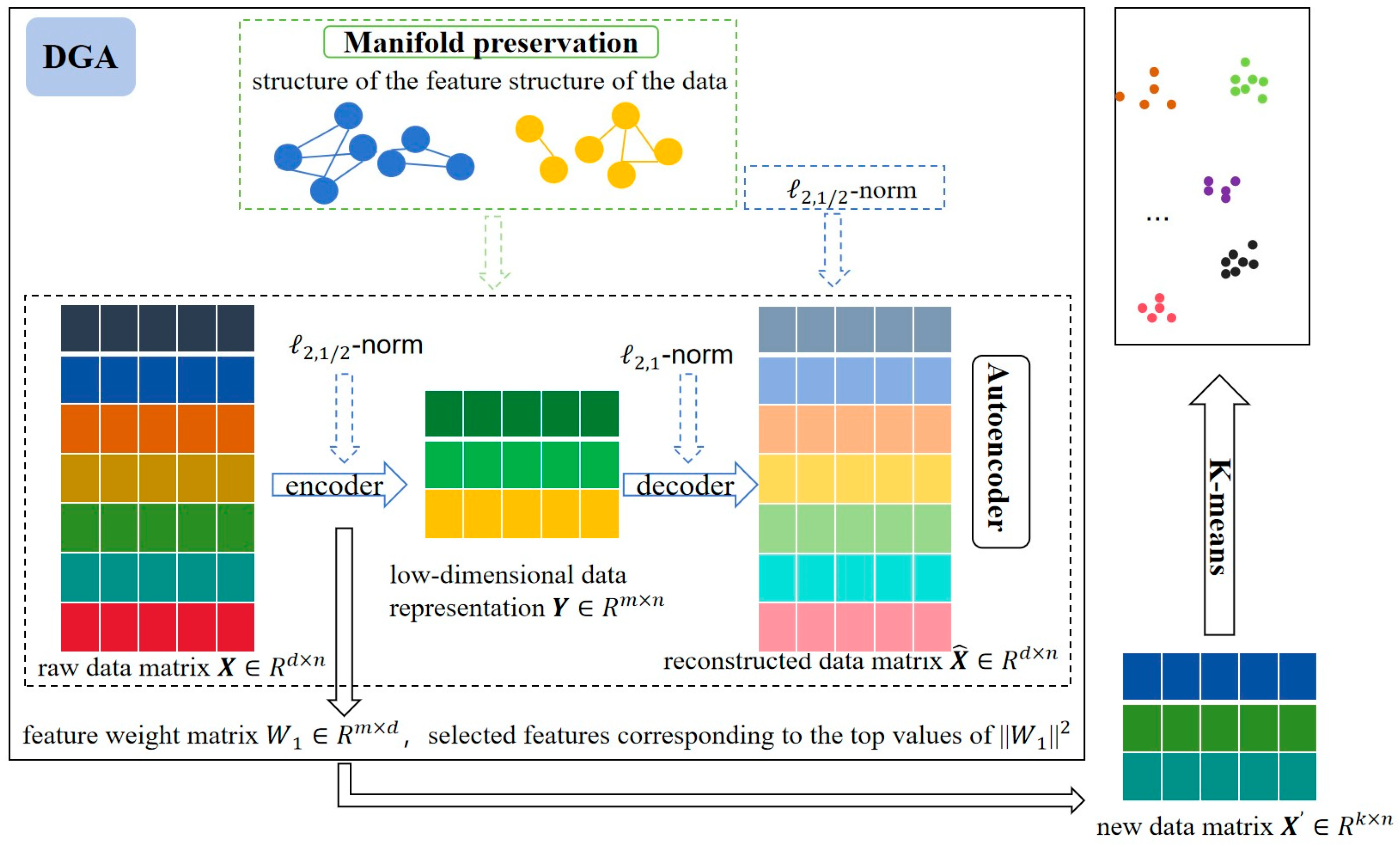
2.4. Proposed Method
2.4.1. Data Reconstruction Based on Autoencoder
2.4.2. Local Structure Preservation Based on Dual-Graph Regularization
2.4.3. Optimization Method
| Algorithm 1. Unsupervised feature selection method based on dual-graph autoencoder (DGA) | |
| Input: | Data matrix hidden layer size: KNN parameter learning rate balance parameters |
| Output: | The selected subset of the features. |
| 1: | Initialize the parameters , , , of auto-encoders; |
| 2: | repeat |
| 3: | Calculate loss of auto-encoder by Equation (17); |
| 4: | Update by Equation (18); |
| 5: | Update the -th diagonal element of D by ; |
| 6: | Update by Equation (23) |
| 7: | Update the jth diagonal element of B by ; |
| 8: | Update by Equation (26); |
| 9: | Update by Equation (27); |
| 10: | until Convergence |
| Return Selected features corresponding to the top k values of ||W1||2, which are sorted by descending order | |
2.4.4. Computational Complexity Analysis
3. Results
3.1. The Experimental Preparation
3.1.1. Datasets
3.1.2. Evaluation Metrics
3.1.3. Algorithms Compared
- Baseline: Select all features;
- LS ([2]): The Laplacian Score approach, which chooses the features with the greatest variance while effectively preserving the local manifold structure of the data;
- SCFS ([12]): Unsupervised feature selection for subspace clustering, using self-expression models to learn cluster similarity to select discriminant features;
- UDFS ([38]): Uses the discriminant information of local structure and l_2,1-norm regularization discriminant to select features;
- MCFS ([13]): Clustering feature selection grounded in spectral analysis and sparse regularization;
- DUFS ([39]): Applies the dependency information among features to the unsupervised feature selection process based on regression;
- NLRL-LE ([10]): A feature selection method via non-convex constraint and latent representation learning with Laplacian embedding;
- LLSRFS ([40]): A unified framework for optimal feature combination combining local structure learning and exponentially weighted sparse regression.
3.1.4. Parameter Selection
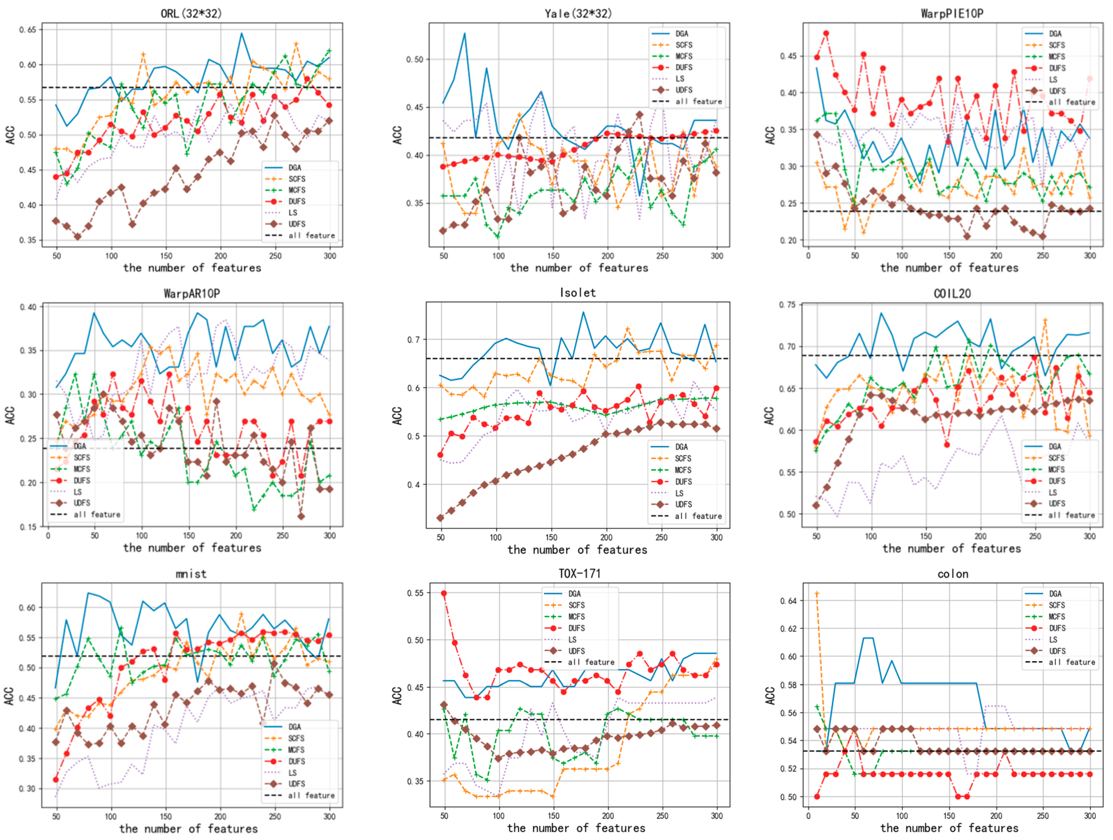
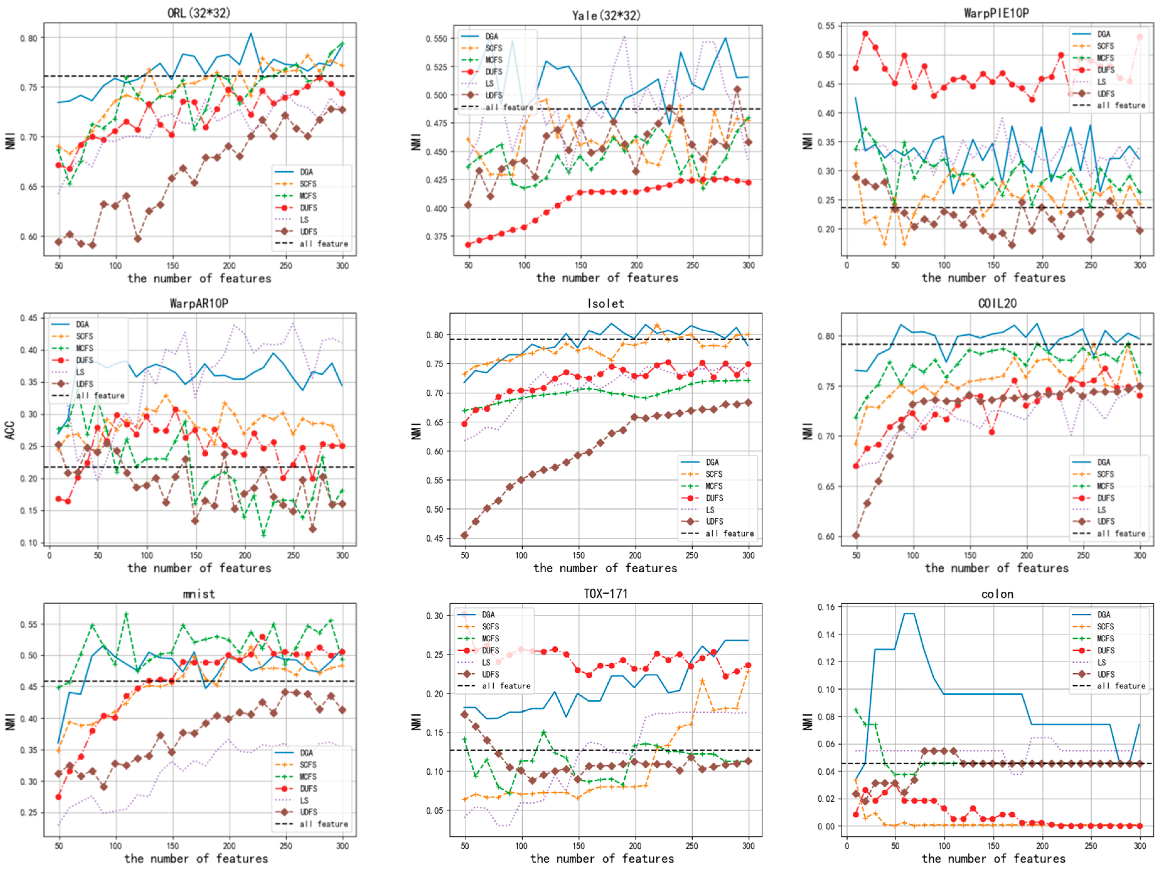
3.2. Classification Results
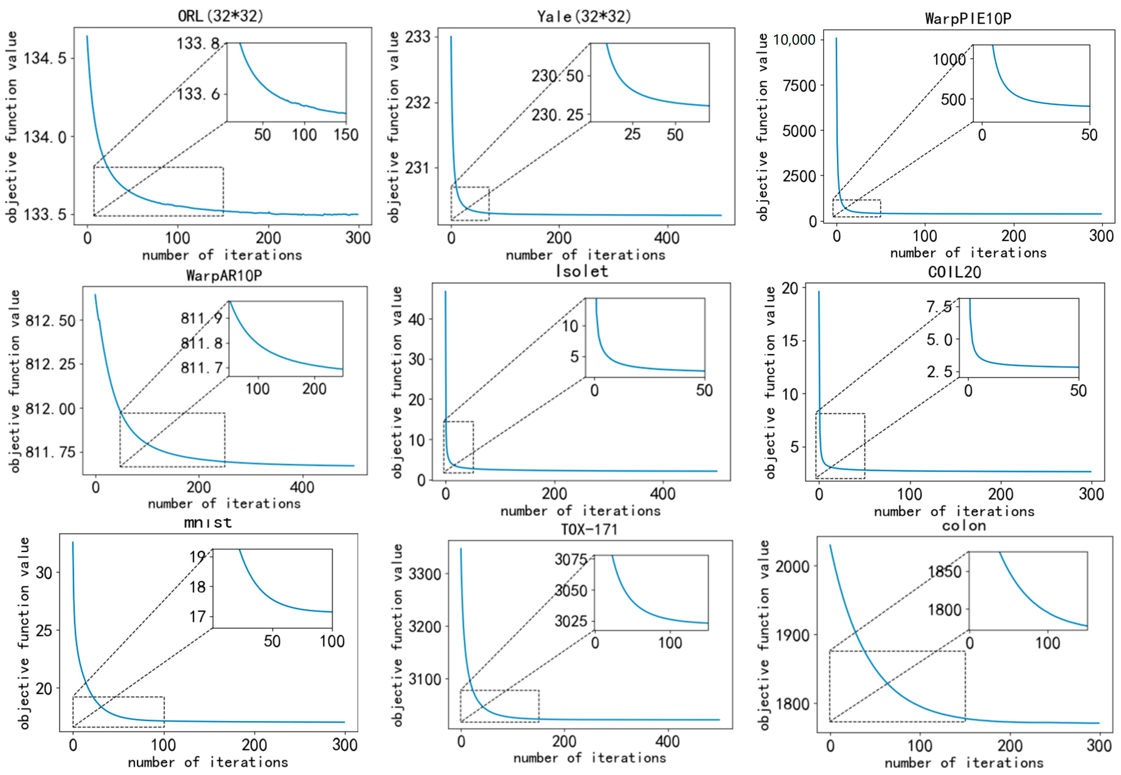
3.3. Convergence Analysis
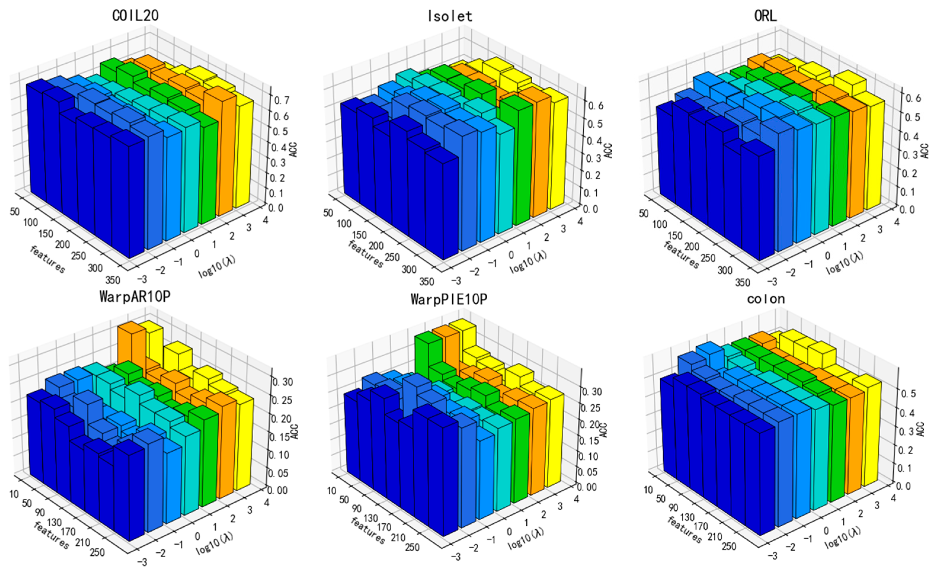
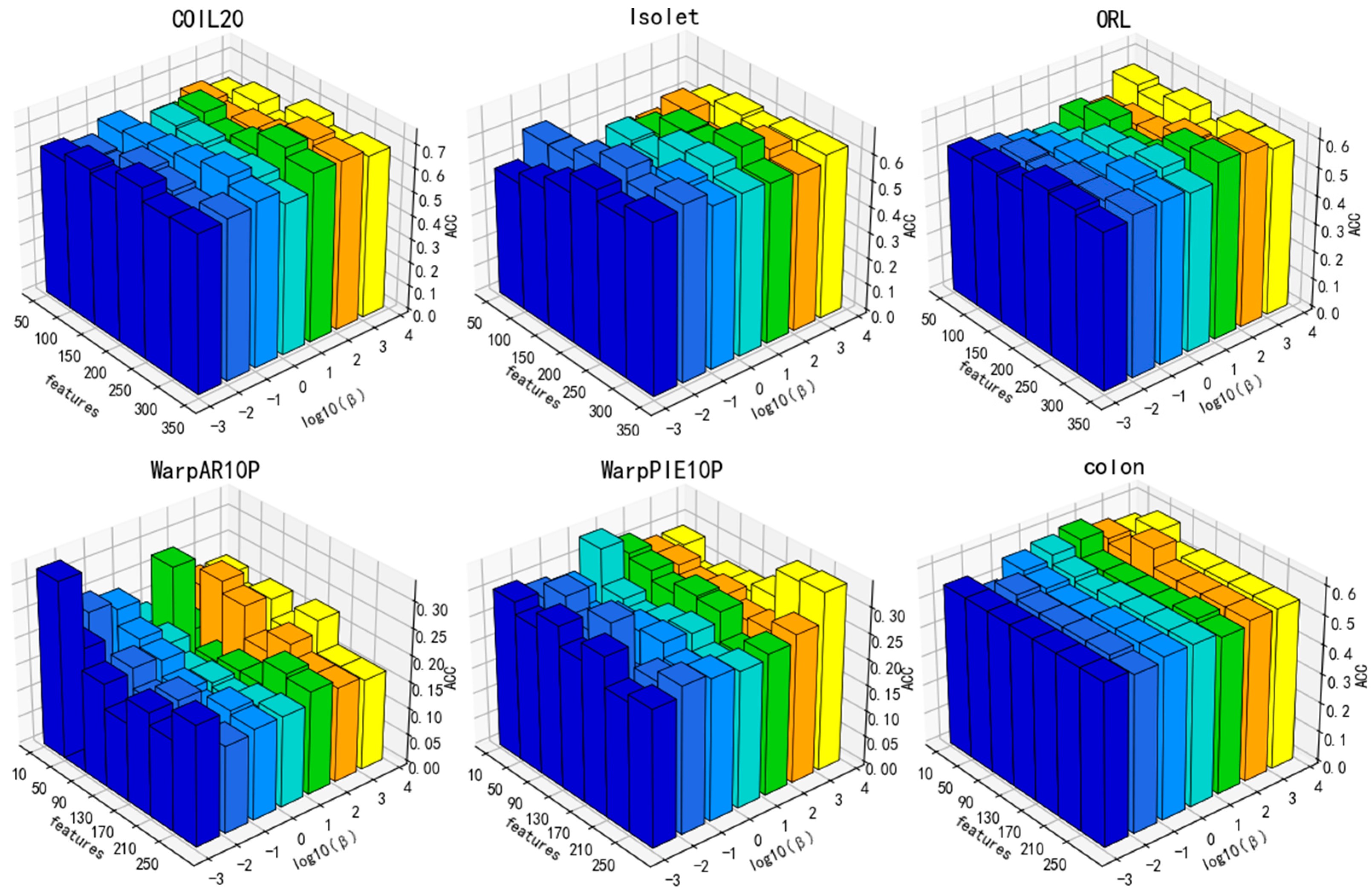
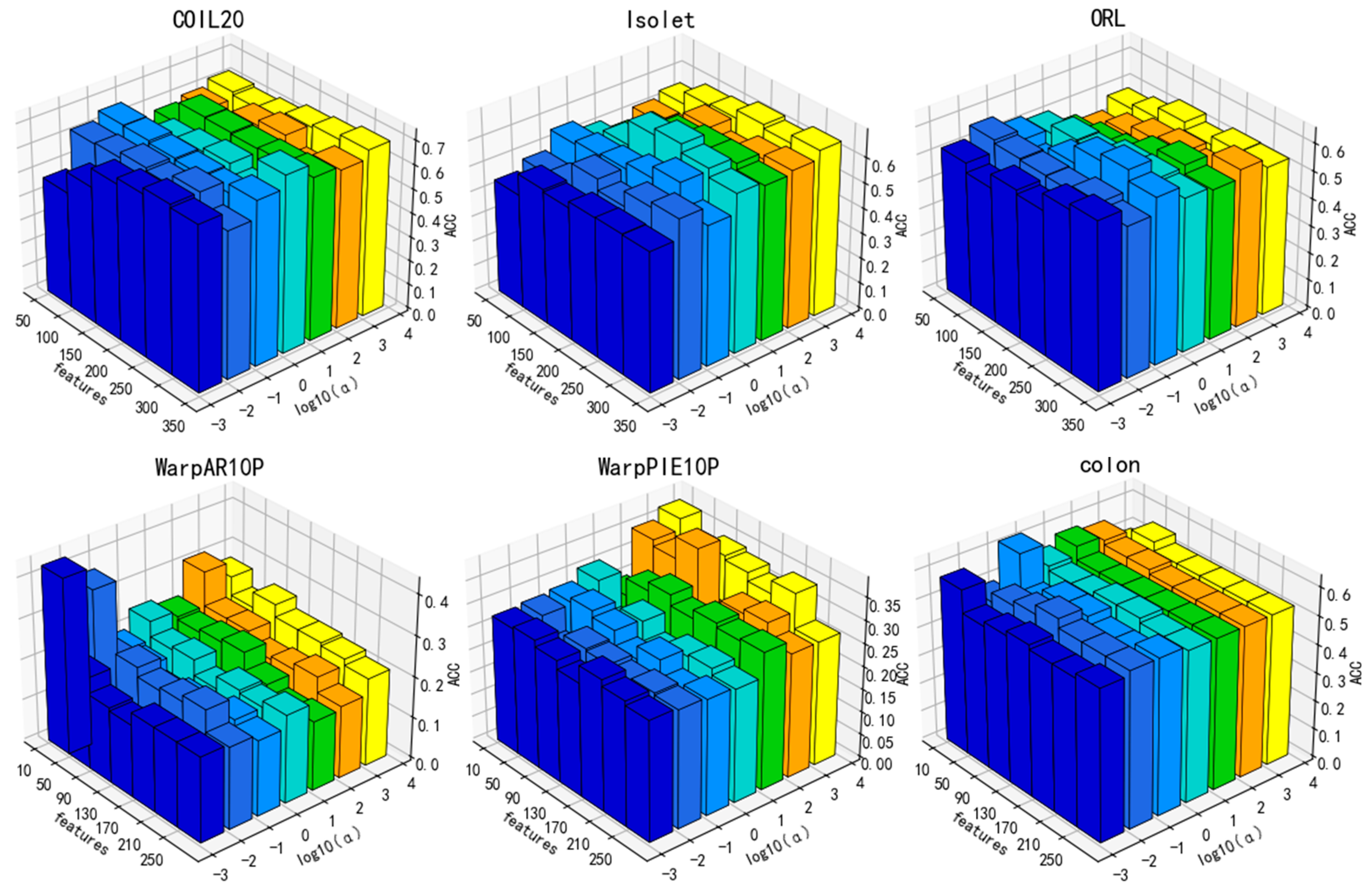
3.4. Parameter Sensitivity Analysis
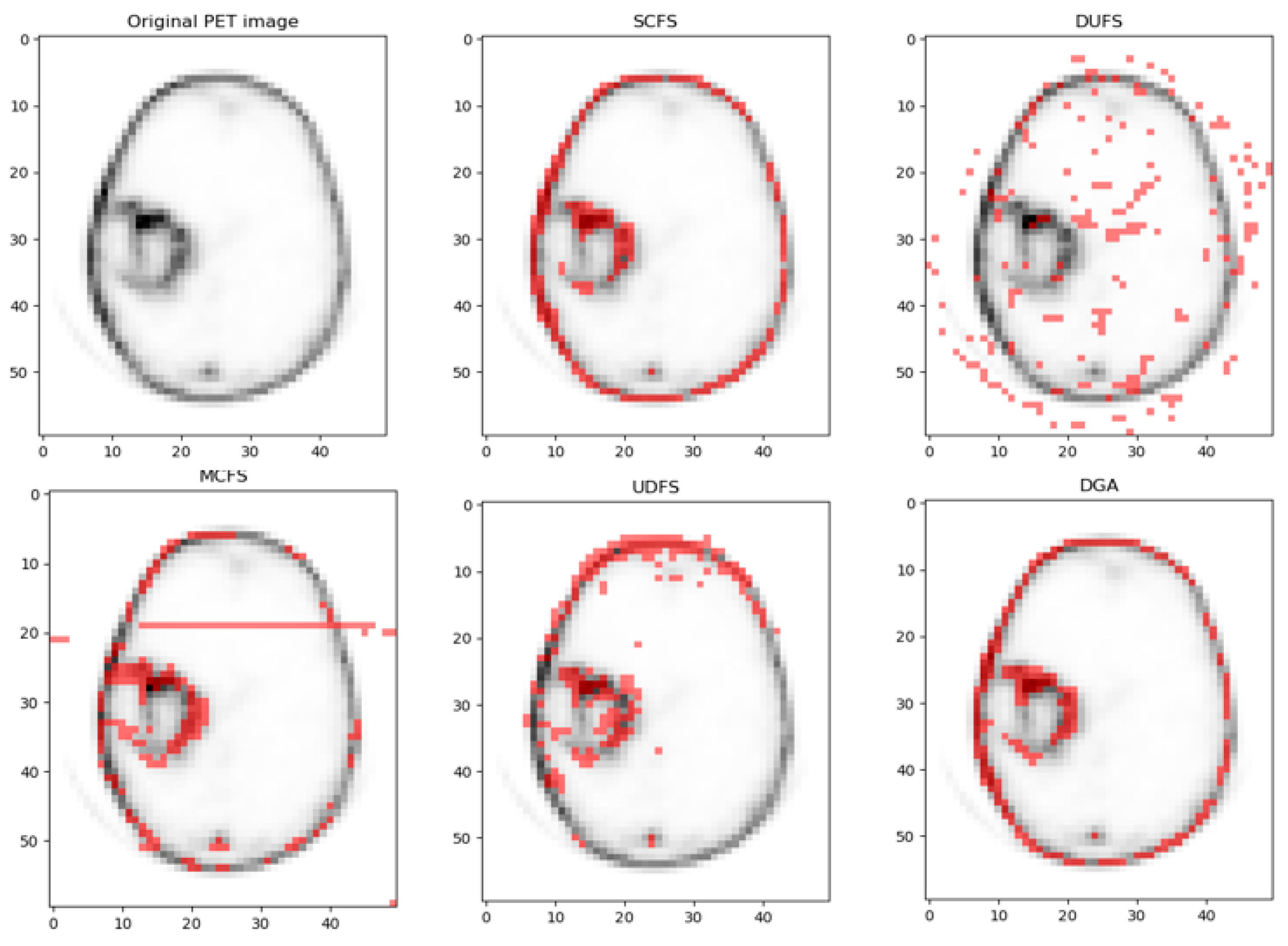
4. Application
4.1. Dataset
4.2. Clustering Evaluation Metrics
- Silhouette Coefficient (SC): The Silhouette Coefficient quantifies how well each sample lies within its cluster compared to other clusters. For a sample , it is defined aswhere is the average intra-cluster distance (compactness) and is the smallest average inter-cluster distance (separation) between sample and all samples in other clusters. The goal SC is the mean of overall samples, ranging from −1 (worst) to 1 (best);
- Davies-Bouldin Index (DBI): The Davies–Bouldin Index evaluates the average similarity between each cluster and its most similar counterpart. It is defined as follows:where is the average distance from samples in cluster to its centroid , and is the distance between centroids and . Lower DBI values indicate better clustering performance.
- Calinski–Harabasz Index (CHI): The Calinski–Harabasz Index measures the ratio of between-cluster dispersion to within-cluster dispersion:where and are the between-cluster and within-cluster covariance matrices, is the number of clusters, and N is the total number of samples. A higher CHI value indicates better-defined clusters.
4.3. Comparing Results
5. Discussion
Author Contributions
Funding
Institutional Review Board Statement
Informed Consent Statement
Data Availability Statement
Conflicts of Interest
References
- Song, L.; Smola, A.; Gretton, A.; Borgwardt, K.M.; Bedo, J. Supervised feature selection via dependence estimation. In Proceedings of the 24th International Conference on Machine Learning, Corvallis, OR, USA, 20–24 June 2007. [Google Scholar]
- Solorio-Fernández, S.; Carrasco-Ochoa, J.A.; Martínez-Trinidad, J.F. A review of unsupervised feature selection methods. Artif. Intell. Rev. 2020, 53, 907–948. [Google Scholar] [CrossRef]
- Zhao, Z.; Liu, H. Semi-supervised feature selection via spectral analysis. In Proceedings of the 2007 SIAM International Conference on Data Mining, Minneapolis, MN, USA, 26–28 April 2007. [Google Scholar]
- Xu, Z.; King, I.; Lyu, M.R.-T.; Jin, R. Discriminative semi-supervised feature selection via manifold regularization. IEEE Trans. Neural Netw. 2010, 21, 1033–1047. [Google Scholar]
- Zhang, L.; Liu, M.; Wang, R.; Du, T.; Li, J. Multi-view unsupervised feature selection with dynamic sample space structure. In Proceedings of the 2019 IEEE Symposium Series on Computational Intelligence (SSCI), Xiamen, China, 6–9 December 2019. [Google Scholar]
- Li, J.; Cheng, K.; Wang, S.; Morstatter, F.; Trevino, R.P.; Tang, J.; Liu, H. Feature selection: A data perspective. ACM Comput. Surv. (CSUR) 2017, 50, 1–45. [Google Scholar] [CrossRef]
- Constantinopoulos, C.; Titsias, M.K.; Likas, A. Bayesian feature and model selection for Gaussian mixture models. IEEE Trans. Pattern Anal. Mach. Intell. 2006, 28, 1013–1018. [Google Scholar] [CrossRef] [PubMed]
- Tabakhi, S.; Moradi, P.; Akhlaghian, F. An unsupervised feature selection algorithm based on ant colony optimization. Eng. Appl. Artif. Intell. 2014, 32, 112–123. [Google Scholar] [CrossRef]
- Zheng, W.; Zhu, X.; Wen, G.; Zhu, Y.; Yu, H.; Gan, J. Unsupervised feature selection by self-paced learning regularization. Pattern Recognit. Lett. 2020, 132, 4–11. [Google Scholar] [CrossRef]
- Shang, R.; Kong, J.; Feng, J.; Jiao, L. Feature selection via non-convex constraint and latent representation learning with Laplacian embedding. Expert Syst. Appl. 2022, 208, 118179. [Google Scholar] [CrossRef]
- Wang, S.; Pedrycz, W.; Zhu, Q.; Zhu, W. Subspace learning for unsupervised feature selection via matrix factorization. Pattern Recognit. 2015, 48, 10–19. [Google Scholar] [CrossRef]
- Parsa, M.G.; Zare, H.; Ghatee, M. Unsupervised feature selection based on adaptive similarity learning and subspace clustering. Eng. Appl. Artif. Intell. 2020, 95, 103855. [Google Scholar] [CrossRef]
- Cai, D.; He, X.; Han, J.; Huang, T.S. Graph regularized nonnegative matrix factorization for data representation. IEEE Trans. Pattern Anal. Mach. Intell. 2010, 33, 1548–1560. [Google Scholar]
- Li, Z.; Yang, Y.; Liu, J.; Zhou, X.; Lu, H. Unsupervised feature selection using nonnegative spectral analysis. In Proceedings of the AAAI Conference on Artificial Intelligence, Toronto, ON, Canada, 22–26 July 2012. [Google Scholar]
- Feng, S.; Duarte, M.F. Graph autoencoder-based unsupervised feature selection with broad and local data structure preservation. Neurocomputing 2018, 312, 310–323. [Google Scholar] [CrossRef]
- Gu, Q.; Zhou, J. Co-clustering on manifolds. In Proceedings of the 15th ACM SIGKDD International Conference on Knowledge Discovery and Data Mining, Paris, France, 28 June 28–1 July 2009. [Google Scholar]
- Shang, F.; Jiao, L.C.; Wang, F. Graph dual regularization non-negative matrix factorization for co-clustering. Pattern Recognit. 2012, 45, 2237–2250. [Google Scholar] [CrossRef]
- Zheng, W.; Yan, H.; Yang, J. Robust unsupervised feature selection by nonnegative sparse subspace learning. Neurocomputing 2019, 334, 156–171. [Google Scholar] [CrossRef]
- Han, K.; Wang, Y.; Zhang, C.; Li, C.; Xu, C. Autoencoder inspired unsupervised feature selection. In Proceedings of the 2018 IEEE International Conference on Acoustics, Speech and Signal Processing (ICASSP), Calgary, AB, Canada, 15–20 April 2018. [Google Scholar]
- Gong, X.; Yu, L.; Wang, J.; Zhang, K.; Bai, X.; Pal, N.R. Unsupervised feature selection via adaptive autoencoder with redundancy control. Neural Netw. 2022, 150, 87–101. [Google Scholar] [CrossRef]
- Wang, S.; Ding, Z.; Fu, Y. Feature selection guided auto-encoder. In Proceedings of the AAAI Conference on Artificial Intelligence, San Francisco, CA, USA, 4–9 February 2017. [Google Scholar]
- Zhang, T.; Chen, W.; Liu, Y.; Wu, L. An intrusion detection method based on stacked sparse autoencoder and improved gaussian mixture model. Comput. Secur. 2023, 128, 103144. [Google Scholar] [CrossRef]
- Manzoor, U.; Halim, Z. Protein encoder: An autoencoder-based ensemble feature selection scheme to predict protein secondary structure. Expert Syst. Appl. 2023, 213, 119081. [Google Scholar]
- Zhang, Y.; Lu, Z.; Wang, S. Unsupervised feature selection via transformed auto-encoder. Knowl.-Based Syst. 2021, 215, 106748. [Google Scholar] [CrossRef]
- Li, X.; Zhang, R.; Wang, Q.; Zhang, H. Autoencoder constrained clustering with adaptive neighbors. IEEE Trans. Neural Netw. Learn. Syst. 2020, 32, 443–449. [Google Scholar] [CrossRef]
- Lu, G.; Leng, C.; Li, B.; Jiao, L.; Basu, A. Robust dual-graph discriminative NMF for data classification. Knowl.-Based Syst. 2023, 268, 110465. [Google Scholar] [CrossRef]
- Yin, M.; Gao, J.; Lin, Z.; Shi, Q.; Guo, Y. Dual graph regularized latent low-rank representation for subspace clustering. IEEE Trans. Image Process. 2015, 24, 4918–4933. [Google Scholar] [CrossRef]
- Shang, R.; Wang, W.; Stolkin, R.; Jiao, L. Non-negative spectral learning and sparse regression-based dual-graph regularized feature selection. IEEE Trans. Cybern. 2017, 48, 793–806. [Google Scholar] [CrossRef] [PubMed]
- Jiang, B.; Ding, C. Revisiting L2,1-norm robustness with vector outlier regularization. IEEE Trans. Neural Netw. Learn. Syst. 2020, 31, 5624–5629. [Google Scholar] [CrossRef] [PubMed]
- Zhu, P.; Xu, Q.; Hu, Q.; Zhang, C. Co-regularized unsupervised feature selection. Neurocomputing 2018, 275, 2855–2863. [Google Scholar] [CrossRef]
- Huang, Q.; Yin, X.; Chen, S.; Wang, Y.; Chen, B. Robust nonnegative matrix factorization with structure regularization. Neurocomputing 2020, 412, 72–90. [Google Scholar] [CrossRef]
- Wang, L.; Chen, S.; Wang, Y. A unified algorithm for mixed l2,p-minimizations and its application in feature selection. Comput. Optim. Appl. 2014, 58, 409–421. [Google Scholar] [CrossRef]
- Shi, Y.; Miao, J.; Wang, Z.; Zhang, P.; Niu, L. Feature selection with ℓ2,1–2 regularization. IEEE Trans. Neural Netw. Learn. Syst. 2018, 29, 4967–4982. [Google Scholar] [CrossRef]
- Li, Z.; Tang, J. Unsupervised feature selection via nonnegative spectral analysis and redundancy control. IEEE Trans. Image Process. 2015, 24, 5343–5355. [Google Scholar] [CrossRef] [PubMed]
- Meng, Y.; Shang, R.; Jiao, L.; Zhang, W.; Yang, S. Dual-graph regularized non-negative matrix factorization with sparse and orthogonal constraints. Eng. Appl. Artif. Intell. 2018, 69, 24–35. [Google Scholar] [CrossRef]
- Li, W.; Chen, H.; Li, T.; Wan, J.; Sang, B. Unsupervised feature selection via self-paced learning and low-redundant regularization. Knowl.-Based Syst. 2022, 240, 108150. [Google Scholar] [CrossRef]
- Nie, F.; Xu, D.; Tsang, I.W.; Zhang, C. Spectral embedded clustering. In Proceedings of the IJCAI International Joint Conference on Artificial Intelligence, Pasadena, CA, USA, 11–17 July 2009. [Google Scholar]
- Yang, Y.; Shen, H.T.; Ma, Z.; Huang, Z.; Zhou, X. ℓ2, 1-norm regularized discriminative feature selection for unsupervised learning. In Proceedings of the IJCAI International Joint Conference on Artificial Intelligence, Barcelona, Spain, 16–22 July 2011. [Google Scholar]
- Lim, H.; Kim, D.-W. Pairwise dependence-based unsupervised feature selection. Pattern Recognit. 2021, 111, 107663. [Google Scholar] [CrossRef]
- Wang, C.; Wang, J.; Gu, Z.; Wei, J.-M.; Liu, J. Unsupervised feature selection by learning exponential weights. Pattern Recognit. 2024, 148, 110183. [Google Scholar] [CrossRef]
- Roustaei, H.; Norouzbeigi, N.; Vosoughi, H.; Aryana, K. A dataset of [68Ga] Ga-Pentixafor PET/CT images of patients with high-grade Glioma. Data Brief 2023, 48, 109236. [Google Scholar] [CrossRef] [PubMed]


| ID | Datasets | Instances | Features | Classes | Data Types | Description |
|---|---|---|---|---|---|---|
| 1 | Isolet [6] | 1560 | 617 | 26 | Image, text | UCI dataset |
| 2 | Mnist [26] | 2000 | 784 | 10 | Image, text | Handwritten digits, 28 × 28 pixels |
| 3 | Yale (32*32) [6] | 165 | 1024 | 15 | Image, Face | Yale face database, 32*32 grayscale |
| 4 | ORL (32*32) [6] | 400 | 1024 | 40 | Image, Face | AT&T face dataset |
| 5 | COIL20 [6] | 1440 | 1024 | 20 | Image, Object | Columbia object images |
| 6 | WarpAR10P [6] | 130 | 2400 | 10 | Image, Face | Cropped face images under different conditions |
| 7 | WarpPIE10P [6] | 210 | 2420 | 10 | Image, Face | PIE face dataset, cropped |
| 8 | Colon [6] | 62 | 2000 | 2 | Gene expression, Biology | Tumor vs. normal colon tissue |
| 9 | TOX-171 [6] | 171 | 5748 | 4 | Gene expression, Biology | Toxicogenomic gene expression data |
| All Features | LS | SCFS | UDFS | MCFS | DUFS | DGA | ||
|---|---|---|---|---|---|---|---|---|
| ACC | Isolet | 0.658 | 0.612 | 0.721 | 0.528 | 0.578 | 0.602 | 0.755 |
| mnist | 0.519 | 0.469 | 0.5895 | 0.507 | 0.566 | 0.5575 | 0.6235 | |
| Yale (32*32) | 0.418 | 0.4667 | 0.442 | 0.442 | 0.406 | 0.419 | 0.527 | |
| ORL (32*32) | 0.5675 | 0.555 | 0.63 | 0.5275 | 0.62 | 0.58 | 0.645 | |
| COIL20 | 0.6889 | 0.617 | 0.731 | 0.637 | 0.707 | 0.686 | 0.739 | |
| WarpAR10P | 0.238 | 0.384 | 0.353 | 0.3 | 0.323 | 0.292 | 0.392 | |
| WarpPIE10P | 0.2621 | 0.385 | 0.323 | 0.342 | 0.371 | 0.48 | 0.433 | |
| colon | 0.532 | 0.564 | 0.645 | 0.548 | 0.564 | 0.548 | 0.612 | |
| TOX-171 | 0.415 | 0.438 | 0.479 | 0.431 | 0.426 | 0.549 | 0.485 | |
| NMI | Isolet | 0.791 | 0.745 | 0.816 | 0.669 | 0.721 | 0.752 | 0.818 |
| mnist | 0.458 | 0.361 | 0.513 | 0.441 | 0.453 | 0.5055 | 0.498 | |
| Yale (32*32) | 0.487 | 0.52 | 0.495 | 0.488 | 0.459 | 0.425 | 0.55 | |
| ORL (32*32) | 0.76 | 0.744 | 0.781 | 0.721 | 0.793 | 0.759 | 0.804 | |
| COIL20 | 0.791 | 0.744 | 0.792 | 0.747 | 0.782 | 0.751 | 0.803 | |
| WarpAR10P | 0.21718 | 0.438 | 0.304 | 0.254 | 0.338 | 0.278 | 0.38 | |
| WarpPIE10P | 0.236 | 0.39 | 0.323 | 0.288 | 0.372 | 0.536 | 0.425 | |
| colon | 0.045797 | 0.06425 | 0.03363 | 0.03122 | 0.08478 | 0.03122 | 0.154 | |
| TOX-171 | 0.127 | 0.169 | 0.228 | 0.173 | 0.141 | 0.301 | 0.267 |
| ACC | NMI | |||||
|---|---|---|---|---|---|---|
| NLRL-LE | LLSRFS | DGA | NLRL-LE | LLSRFS | DGA | |
| Isolet | 0.7071 ± 0.0201 | 0.6517 ± 0.0067 | 0.7472 ± 0.0114 | 0.7869 ± 0.0104 | 0.7848 ± 0.0052 | 0.812 ± 0.004 |
| mnist | 0.5765 ± 0.0142 | - | 0.6172 ± 0.0042 | 0.4986 ± 0.006 | - | 0.5004 ± 0.0039 |
| Yale (32*32) | - | 0.4856 ± 0.0040 | 0.5054 ± 0.0124 | - | 0.5652 ± 0.0062 | 0.5442 ± 0.0061 |
| ORL (32*32) | - | 0.6113 ± 0.0073 | 0.632 ± 0.0154 | - | 0.7930 ± 0.0056 | 0.7920 ± 0.0071 |
| COIL20 | 0.6797 ± 0.0406 | 0.7357 ± 0.0053 | 0.743 ± 0.021 | 0.7742 ± 0.0180 | 0.8335 ± 0.0024 | 0.8085 ± 0.0036 |
| WarpAR10P | - | - | 0.3785 ± 0.0049 | - | - | 0.3645 ± 0.0190 |
| WarpPIE10P | 0.5357 ± 0.0256 | - | 0.4238 ± 0.0158 | 0.5666 ± 0.0235 | - | 0.3994 ± 0.0173 |
| colon | - | - | 0.608 ± 0.004 | - | - | 0.100 ± 0.029 |
| TOX-171 | 0.5465 ± 0.0150 | 0.5268 ± 0.0174 | 0.468 ± 0.062 | 0.2295 ± 0.0157 | 0.3574 ± 0.0076 | 0.206 ± 0.027 |
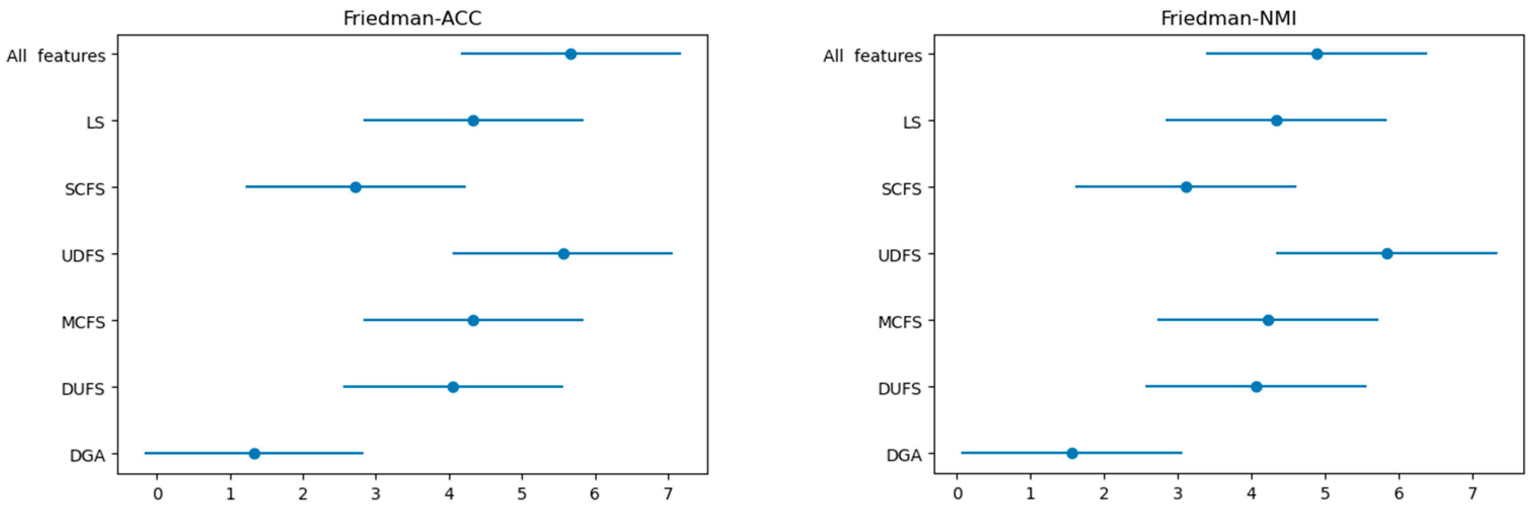
| ) (1.9006) | Nemenyi Post Hoc Test (CD) | |
|---|---|---|
| ACC | = 8.192771084337322 | CD = 2.742416965892462 |
| NMI | = 5.23896388179497 | CD = 2.742416965892462 |
| Method | SC | CHI | DBI |
|---|---|---|---|
| Baseline | 0.21 ± 0.03 | 152.3 ± 12.1 | 1.98 ± 0.15 |
| SCFS | 0.28 ± 0.04 | 198.6 ± 15.7 | 1.67 ± 0.13 |
| UDFS | 0.30 ± 0.03 | 223.1 ± 16.9 | 1.53 ± 0.09 |
| MCFS | 0.35 ± 0.02 | 268.4 ± 20.3 | 1.38 ± 0.08 |
| DUFS | 0.31 ± 0.03 | 234.5 ± 17.6 | 1.49 ± 0.10 |
| DGA | 0.41 ± 0.02 | 275.8 ± 22.5 | 1.12 ± 0.07 |
Disclaimer/Publisher’s Note: The statements, opinions and data contained in all publications are solely those of the individual author(s) and contributor(s) and not of MDPI and/or the editor(s). MDPI and/or the editor(s) disclaim responsibility for any injury to people or property resulting from any ideas, methods, instructions or products referred to in the content. |
© 2025 by the authors. Licensee MDPI, Basel, Switzerland. This article is an open access article distributed under the terms and conditions of the Creative Commons Attribution (CC BY) license (https://creativecommons.org/licenses/by/4.0/).
Share and Cite
Song, Z.; Chen, M.; Xie, L.; Fang, X.
Unsupervised Feature Selection via a Dual-Graph Autoencoder with
Song Z, Chen M, Xie L, Fang X.
Unsupervised Feature Selection via a Dual-Graph Autoencoder with
Song, Zhichao, Meiling Chen, Liang Xie, and Xi Fang.
2025. "Unsupervised Feature Selection via a Dual-Graph Autoencoder with
Song, Z., Chen, M., Xie, L., & Fang, X.
(2025). Unsupervised Feature Selection via a Dual-Graph Autoencoder with