Prediction Method of Tangerine Peel Drying Moisture Ratio Based on KAN-BiLSTM and Multimodal Feature Fusion

Abstract

Tangerine peel, rich in moisture (75–90%) and medicinal value, requires drying to prevent spoilage and extend shelf life. Traditional heat pump drying often causes uneven airflow, leading to inconsistent drying and nutrient loss, compromising product quality and storage stability. In this study, a prediction model of drying moisture ratio of tangerine peel based on Kolmogorov–Arnold network bidirectional long short-term memory (KAN-BiLSTM) and multimodal feature fusion is proposed. A pre-trained visual geometry group U-shaped network (VGG-UNet) is employed to segment tangerine peel images and extract color, contour, and texture features, while airflow distribution is simulated using finite element analysis (FEA) to obtain spatial location information. These multimodal features are fused and input into a KAN-BiLSTM model, where the KAN layer enhances nonlinear feature representation and a multi-head attention (MHA) mechanism highlights critical temporal and spatial features to improve prediction accuracy. Experimental validation was conducted on a dataset comprising 432 tangerine peel samples collected across six drying batches over a 480 min period, with image acquisition and mass measurement performed every 20 min. The results showed that the pre-trained VGG-UNet achieved a mean intersection over union (MIoU) of 93.58%, outperforming the untrained model by 9.41%. Incorporating spatial features improved the coefficient of determination (R²) of the time series model by 0.08 ± 0.04. The proposed KAN-BiLSTM model achieved a mean absolute error (MAE) of 0.024 and R² of 0.9908, significantly surpassing baseline models such as BiLSTM (R² = 0.9049, MAE = 0.0476) and LSTM (R² = 0.8306, MAE = 0.0766), demonstrating superior performance in moisture ratio prediction.

1. Introduction

Citrus is one of the most widely consumed fruits globally and is favored by consumers due to its health benefits and nutritional value. According to the Food and Agriculture Organization of the United Nations (FAO) report, global citrus production reached 76,292,600 tons in 2019, while citrus processing amounted to 16,939,000 tons [1,2]. Tangerine peel, a by-product of citrus processing, is a valuable Chinese herbal medicine with broad application prospects owing to its medicinal properties. However, the high moisture content (75–90%) of tangerine peel limits its storage duration, creating opportunities for microbial spoilage, fermentation, and chemical degradation within a short period [3]. Drying is a pivotal process in food processing, agricultural preservation, and biopharmaceutical manufacturing, where precise control directly affects product quality and energy efficiency [4]. For instance, in tangerine peel drying, traditional heat pump drying equipment exhibits a dynamic and nonlinear process. Uneven airflow distribution may lead to local over-drying or under-drying, resulting in the loss of active ingredients and diminished nutritional quality [5].

Traditional contact moisture measurement methods, such as gravimetric analysis, offer high accuracy but suffer from drawbacks including poor real-time performance and sample destruction [6]. Artificial intelligence (AI) technologies can address these control challenges by optimizing the drying process, establishing robust predictive models, and ultimately yielding high-quality products [7]. Consequently, researchers have proposed moisture prediction models based on image analysis and environmental parameters to validate the feasibility of non-contact methods [8]. Nevertheless, although non-contact detection techniques such as near-infrared spectroscopy [9] and computer vision [7,10] have been applied, among these, near-infrared spectroscopy stands out due to its ability to characterize the responses of C–H, O–H, and N–H groups in organic molecules, enabling rapid analysis of material structure, composition, and concentration [9]. However, single-modal data are often insufficient to fully capture the spatiotemporal dynamics of the drying process.

In recent years, machine learning techniques have demonstrated unique advantages in drying modeling and dynamic control through the integration of sensor data and multi-objective optimization algorithms [11]. For instance, Song improved tea moisture prediction accuracy to 92.5% by combining near-infrared spectroscopy with environmental parameters, although dynamic flow field information was not included [9]. These methods provide new strategies to overcome limitations such as the inadequate accuracy of traditional contact measurements and quality fluctuations caused by uneven airflow. Long short-term memory networks (LSTM) employ gating mechanisms that selectively retain or discard information from the cell state, enabling the effective simulation of complex drying dynamics [12]. Existing methods, including LSTM and variants of LSTM, have been applied to predict moisture content, but most approaches lack integration with dynamic environmental data, such as airflow distribution, leading to limitations in capturing the complex spatiotemporal patterns in the drying process [13,14]. Bidirectional LSTM (BiLSTM) architecture demonstrates exceptional capability in modeling long-range temporal dependencies within sequential data, as evidenced by Qiu’s innovative integration of attention mechanisms with BiLSTM networks, which achieved notable improvement in trend pattern recognition for oil production forecasting in well operations [15]. Convolutional neural networks (CNN) have also excelled in image feature extraction; for example, Wang employed a visual geometry group U-shaped network (VGG-UNet) for yarn curling detection, successfully extracting structural features and providing methodological support for visual-driven drying monitoring [16]. However, their application in drying has mostly been limited to offline image analysis, lacking real-time fusion with dynamic environmental parameters.

Computational fluid dynamics (CFD) simulations can accurately model fluid flow, heat transfer, and mass transfer within drying chambers, revealing spatial heterogeneity in air velocity and temperature that drives uneven drying [17]. Pentamwa used CFD to simulate the flow field within a drying chamber and optimize its configuration, thereby significantly improving drying uniformity [18]. Yet, to date, CFD outputs have seldom been fused with machine learning frameworks, leaving a gap between physical simulation data and data-driven prediction models.

The Kolmogorov–Arnold network (KAN) enhances nonlinear representation by replacing traditional linear weights with B-spline-based activation functions, thereby offering greater flexibility in modeling high-dimensional, strongly nonlinear relationships—characteristics typical of coupled airflow–material interactions during drying [4]. For instance, Wu applied KAN to hyperspectral image classification by integrating it with CNN, resulting in a 33.58% reduction in background reconstruction error during hyperspectral anomaly detection and achieving an accuracy improvement of 3.88% over traditional multilayer perceptron (MLP) methods [19]. Similarly, enhanced CNN architecture via KAN attained 98.38% accuracy in gesture recognition tasks [20]. While KAN has shown success in domains such as hyperspectral image classification and gesture recognition, its application to drying kinetics modeling is unprecedented; here, its capacity to learn complex spatiotemporal dynamics is particularly advantageous.

To address these challenges, we propose a novel multimodal fusion strategy that combines CFD-derived airflow and temperature fields with image-based features for moisture prediction. This study hypothesizes that combining visual features with airflow simulation data in a multimodal framework will significantly improve the accuracy of moisture prediction during drying. Central to our approach is the integration of a KAN with a BiLSTM. A semantic segmentation model based on VGG-UNet extracts microscopic features, such as tangerine peel color and texture [16], while finite element analysis (FEA) quantifies the spatial heterogeneity of airflow velocity and temperature distribution inside the drying chamber. This fusion strategy overcomes the limitations of traditional single-modal models. Ultimately, this model provides a valuable reference for the design of efficient drying processes. Therefore, this study aims to propose a Kolmogorov–Arnold network bidirectional long short-term memory (KAN-BiLSTM) neural network model to enhance input feature representation and develop a more accurate predictive model for the tangerine peel moisture ratio.

The main contributions and innovations of this study are summarized as follows:

• Multimodal dataset construction: A comprehensive dataset was developed by synchronously collecting mass loss data and high-resolution images of tangerine peel under controlled drying conditions. This enabled detailed spatiotemporal analysis of drying kinetics and morphological evolution;
• Airflow distribution analysis: In traditional heat pump drying, uneven airflow distribution in the drying chamber results in varying drying rates and uneven moisture content. Finite element analysis was employed to simulate airflow distribution and quantify its impact on drying performance, thereby providing insights into addressing uneven drying;
• Enhanced image segmentation: By integrating a pre-trained VGG encoder into the UNet architecture, the segmentation model achieved superior accuracy and robustness, enabling precise extraction of peel contours under complex backgrounds;
• Novel moisture prediction model: A novel KAN-BiLSTM model was proposed to predict moisture ratio by fusing image features and temperature data. The model demonstrated high performance, with an MAE of 0.024 and R² of 0.9908, indicating excellent nonlinear feature learning capabilities.

2. Materials

2.1. Test Material

In this experiment, fresh tangerines with intact appearance, uniform size, and no signs of decay were selected as the research subjects. Prior to the experiment, the tangerines were stored in a refrigerator at (4 ± 0.5) °C to maintain freshness. During the experiment, the samples were brought to room temperature by placing them in a test chamber maintained at (21 ± 1) °C. The remaining tangerine samples were selected from Citrus reticulata (mandarin), with a diameter ranging from 6.0 to 8.0 cm and an average weight between approximately 120 g and 180 g. To ensure consistency in size and color, only samples with uniform maturity were selected, exhibiting color values in the range of L* 60–75, a* 10–25, and b* 45–60, corresponding to yellow to yellowish-orange peels with occasional light green areas.

2.2. Instrumentation

A QHX-1800BE artificial climate test chamber (Changge Mingtu Machinery Equipment Co., Ltd., Guangzhou, China) was used for segmented variable-temperature drying. The chamber supports PID control with a temperature and humidity accuracy of 0.1 °C and 0.1%, respectively. It is equipped with nine fluorescent lamps for illumination. The specific parameters of the device are listed in

Table 1. Specifications of the QHX-1800BE artificial climate test chamber.

Project	Unit	Parameters
Model		QHX-1800BE
Working Temperature	°C	1–70
Working Humidity	RH (%)	0–99%
Power Supply	V	220
Inner Size	mm	700 × 500 × 1130
Material Layer Size	mm	660 × 470
Power	kW	1.8
Lighting	LUX	0–20,000

.

Additional instruments used include a Leqi CZ3003 electronic analytical balance (Dongguan Meidi Electronic Technology Co., Ltd., Foshan, China) (measuring range: 500 g; precision: 0.001 g), a digital camera, and a custom scaffold for image capture.

2.3. Test Method

2.3.1. Screening Samples

Tangerine peel samples showing defects such as sunburn, oil spots, brown spots, disease, or insect damage, covering more than 15% of the surface area, were discarded. All selected tangerine peel samples were thoroughly washed with water.

2.3.2. Test Procedure

Initially, the cleaned tangerine peel samples were placed in a test box maintained at 21 °C with an airflow of 1 m/s. Once the surfaces of the tangerine peel samples were adequately dried, the tangerine peel samples were carefully opened. Each tangerine peel sample was oriented with the pedicle side downward. Using a knife, three vertical cuts were made from the tangerine peel samples apex to the pedicle, such that the base remained connected, resulting in three uniform segments (see Figure 1).

After the tangerine peel samples had been opened, the test chamber conditions were adjusted to a fixed temperature of 21 °C, a wind speed of 0.5 m/s, and an illumination level of 5000 LUX. The opened tangerine peel samples were then placed in the test chamber to facilitate dehydration and softening. Once the texture had softened, the tangerine peel samples were inverted so that the inner epidermis faced outward. The test steps and parameters are listed in

Table 2. Test steps and parameters.

Steps	Parameter	Method
Screening Samples		Reject the failed samples; then wash the qualified tangerine peel samples.
Opening Samples	Temperature: 21 °C; Wind Speed: 1 m/s.	Tangerine peel samples were oriented with the pedicle side downward. Using a knife, three vertical cuts were made from the tangerine peel samples apex to the pedicle such that the base remained connected, resulting in three uniform segments.
Flipping Samples	Temperature: 21 °C; Humidity: 60%; Wind Speed: 0.5 m/s; Illumination: 5000 LUX.	The opened tangerine peel samples were then placed in the test chamber to facilitate dehydration and softening. Once the texture had softened, the tangerine peel samples were inverted so that the inner epidermis faced outward.
Drying	Temperature: 45 °C; Wind Speed: 0.5 m/s.	A single layer of tangerine peel was uniformly arranged on the material rack to ensure full coverage, after which the rack was inserted into the drying chamber.

.

2.3.3. Drying Test Design

Prior to the drying tests, the drying chamber was preheated to 60 °C. A single layer of tangerine peel was uniformly arranged on the material rack to ensure full coverage, after which the rack was inserted into the drying chamber. The chamber temperature was then adjusted to 45 °C with a wind speed maintained at 0.5 m/s. Each drying batch consisted of 72 tangerine peel samples. Once drying commenced, the moisture content of the tangerine peel was measured every 20 min, and the corresponding spatial position of each sample was recorded. Simultaneously, images of the tangerine peel were captured using a fixed shooting distance of 25 cm, ensuring a consistent lighting environment throughout the process. For each time point, nine tangerine peels—selected for their uniform size and color—were photographed, and immediately returned to the drying chamber upon completion of the imaging. Drying was terminated when the moisture content stabilized. The entire procedure was repeated across six independent batches, resulting in a total of 432 tangerine peel samples used in this study. In order to ensure experimental rigor, the entire procedure was repeated three times, and the mean values were calculated for subsequent analysis.

2.4. Test Evaluation Index

2.4.1. Water Content

The moisture content of the tangerine peel during drying was calculated using Equation (1) [21]:

$$M_t={\displaystyle \frac{m_t-m_0}{m_0}}$$

(1)

In Equation (1), $M_t$ represents the dry basis moisture content of the tangerine peel at time t (g/g), $m_t$ denotes the mass of the tangerine peel at time t(g), and $m_0$ is the dry basis mass of the tangerine peel (g).

2.4.2. Moisture Ratio

Moisture ratio is a critical parameter for assessing changes in moisture content during the drying process, as it reflects both the degree of drying and the drying rate. The initial calculation is given by Equation (2) [21,22]:

$$M_R={\displaystyle \frac{M_t-M_e}{M_0-M_e}}$$

(2)

Here, M_e is the equilibrium dry basis moisture content (g/g). Given that M_e is typically much smaller than both M_t and M₀, and considering the difficulties in accurately determining M_e under current experimental conditions, it is often neglected. Thus, the moisture ratio (M_R) can be simplified to Equation (3) [22]:

$$M_R={\displaystyle \frac{M_t}{M_0}}$$

(3)

In Equation (3), M₀ denotes the initial dry basis moisture content of the material (g/g).

3. Methods

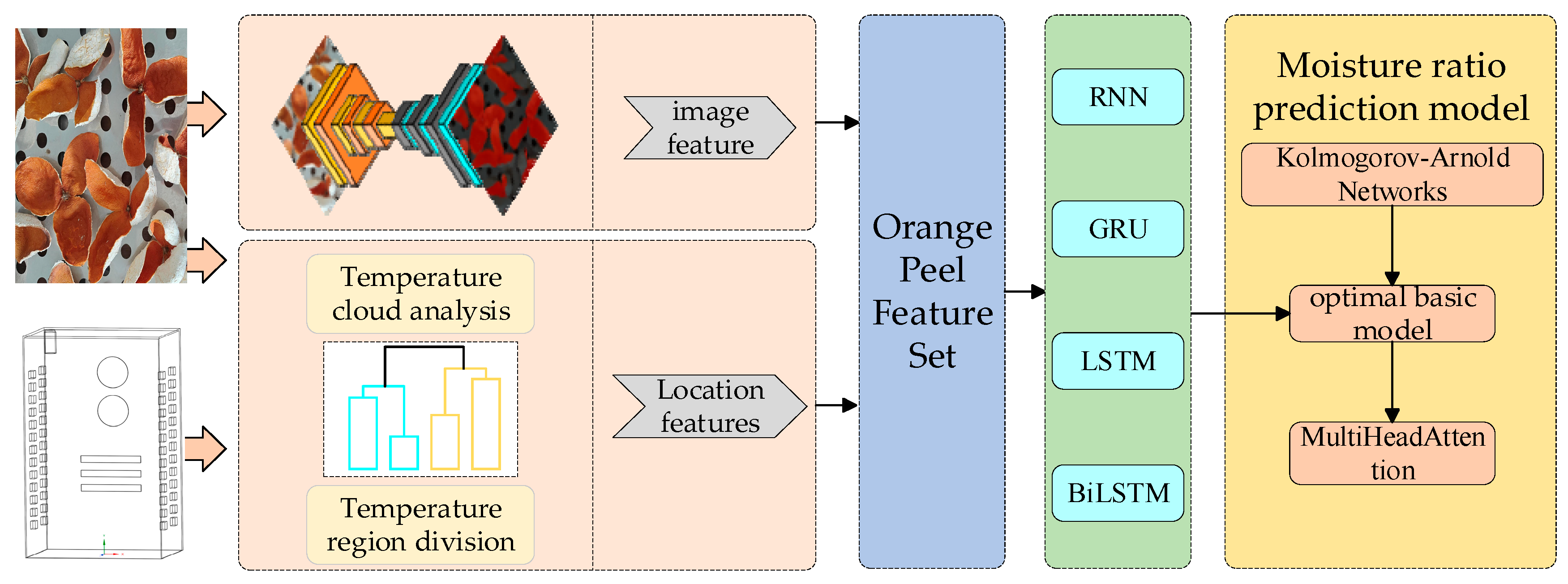
The research framework for this study is illustrated in Figure 2. In this work, we propose a prediction method for the drying moisture ratio of tangerine peel based on a fusion of the KAN-BiLSTM model and multimodal feature fusion. In the proposed approach, a pre-trained VGG-UNet semantic segmentation model was employed to process tangerine peel images and extract features such as color, contour, and texture. Simultaneously, spatial position information was obtained by simulating the airflow distribution within the drying chamber using finite element analysis. Based on these inputs, a KAN-BiLSTM neural network model was constructed, wherein a KAN layer served as the primary feature extraction module. Furthermore, a multi-head attention (MHA) mechanism was embedded between the BiLSTM layer and the fully connected layer to emphasize key temporal steps and salient features, thereby ensuring high-precision prediction.

3.1. Tangerine Peel Spatial Position Feature Extraction

3.1.1. Physical Model of Drying Chamber

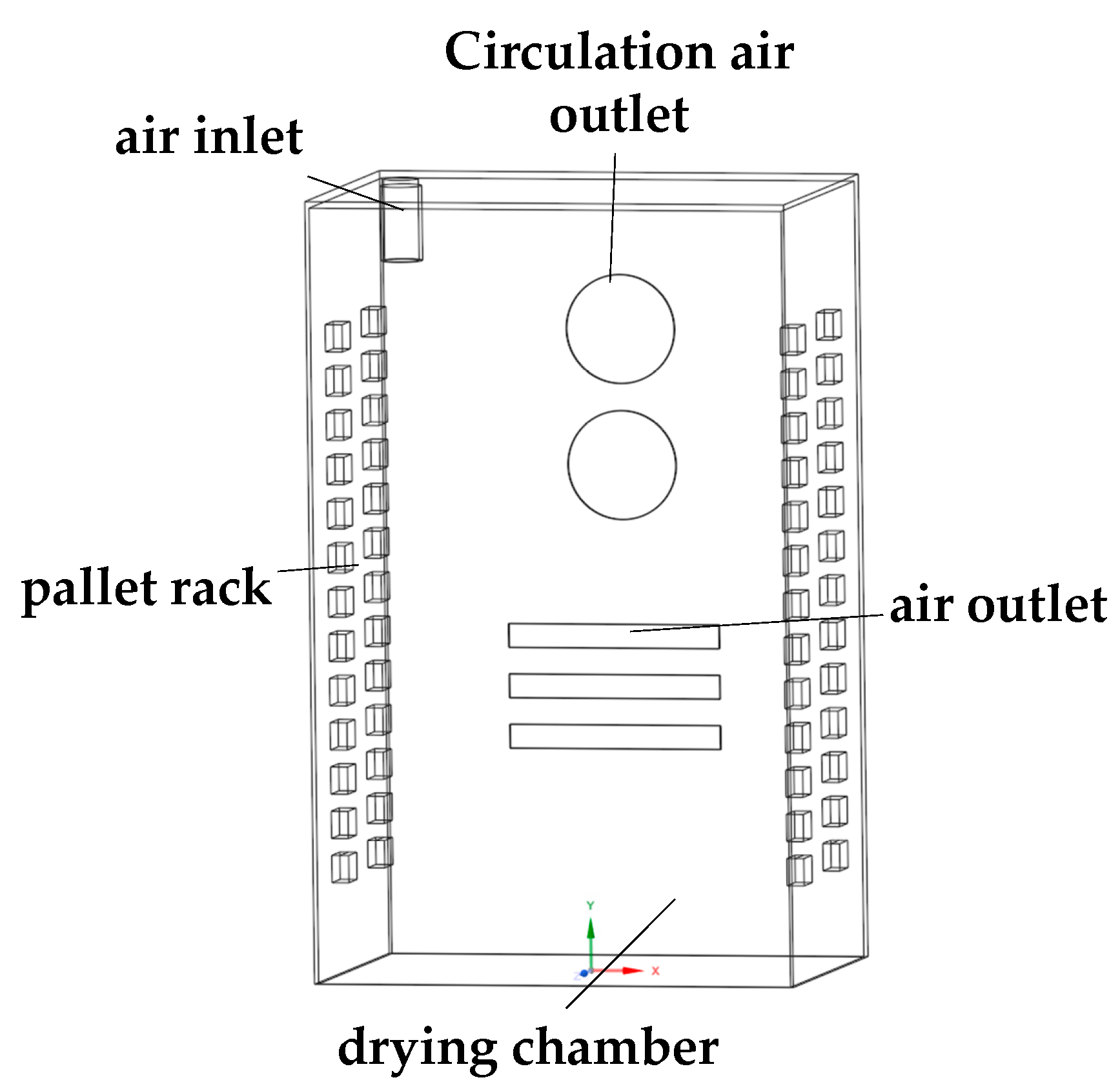
For this study, the QHX-1800BE artificial climate test chamber (manufactured by Changge Mingtu Machinery Equipment Co., Ltd., Guangzhou, China) was used as the experimental drying chamber. An air inlet with a radius of 50 mm was located in the upper left portion of the chamber, and two circulating fans were installed in the central region, each with a tuyere radius of 160 mm. The physical model of the drying chamber is presented in Figure 3.

A three-dimensional model of the drying chamber was created using SpaceClaim 2022 R1 software at a 1:1 scale. In order to streamline the modeling process, the material rack, tray, and the material itself were combined and represented as a single material layer, repeated across all 12 layers. The Ansys meshing module was then employed to discretize the model for computational simulation of the internal temperature distribution and airflow in the heat pump drying chamber. A mesh resolution of 5 mm was adopted, and high grid quality was ensured by setting the mesh smoothness to a high level. Additionally, the regions corresponding to the inlet, outlet, and circulating air outlet were refined (double-encrypted), resulting in a total of 6,970,157 mesh units.

3.1.2. Mathematical Model of Drying Chamber

The mathematical model of the drying chamber was developed using ANSYS Fluent (2022 R1), SpaceClaim (2022 R1), Meshing (2022 R1), and other simulation tools to investigate the heat transfer and airflow mechanisms within the chamber during the drying process. In this model, it is assumed that the flow field in the drying chamber is a steady-state viscous flow [23]. The simulation is based on a standard turbulence model [24], and the energy equation [18] is expressed as Equation (4):

$${\displaystyle \frac{\partial \left(\rho \phi \right)}{\partial t}}+{\displaystyle \frac{\partial \left(\rho u\phi \right)}{\partial }}+{\displaystyle \frac{\partial \left(\rho \upsilon \phi \right)}{\partial }}+{\displaystyle \frac{\partial \left(\rho \omega \phi \right)}{\partial }}={\displaystyle \frac{\partial }{\partial x}}(\Gamma {\displaystyle \frac{\partial \phi }{\partial x}})+{\displaystyle \frac{\partial }{\partial y}}(\Gamma {\displaystyle \frac{\partial \phi }{\partial y}})+{\displaystyle \frac{\partial }{\partial z}}(\Gamma {\displaystyle \frac{\partial \phi }{\partial z}})+S$$

(4)

Here: $\phi$—generalized variable; $\Gamma$—diffusion coefficient; $S$—source item; $\rho$—density; t—time; $u$—x-direction velocity; $\upsilon$—y-direction velocity; $\omega$—z-direction velocity.

For the boundary conditions, a velocity inlet was implemented, with the inlet direction set perpendicular to the boundary and the velocity distributed uniformly. The wind speed was fixed at 0.5 m/s, and the turbulence intensity was estimated to be 3.8% using an empirical formula [10]. The inlet temperature was maintained at 313.15 K (40 °C), and a pressure step of 12 Pa was applied for the circulating fan. The outlet was defined as a free outflow boundary to ensure that all hot air exited the chamber completely. Solid walls were treated with a non-slip condition, and their temperature was set to 25 °C. The coordinate system was configured with the center of the bottom surface of the drying chamber as the origin. Figure 4 shows the volume rendering and temperature cloud distributions on the planes at y = 0.8, y = 0.535, and y = 0.35 as calculated by Fluent, while the top views of these planes are depicted in Figure 5. The velocity inlet was selected as the boundary condition. The inlet direction is perpendicular to the boundary and evenly distributed. The wind speed was set to 0.5 m/s, and the turbulence value was estimated to be 3.8% by the empirical formula [10]. The inlet temperature was 313.15 K (40 °C), and the pressure step of the circulating fan was 12 Pa. The outlet condition was set to free outflow, and the hot air at the outlet flows completely from the outlet. The solid wall used a non-slip condition, and the wall temperature was 25 °C. The coordinate axis was set as shown in the figure, and the center of the bottom surface of the drying chamber was the origin. The volume rendering diagram and the temperature cloud distribution on the surface of y = 0.8, y = 0.535, and y = 0.35 calculated by Fluent are shown in Figure 3. The top view of each plane is shown in Figure 5.

The temperature cloud maps of the upper, middle, and lower layers clearly reveal noticeable temperature gradients, indicating significant temperature differences across different vertical positions within the drying chamber.

3.1.3. Temperature Field Analysis and Region Division

Hierarchical clustering was employed in this study to segment the temperature field into distinct regions. The temperature cloud map data points were extracted as coordinate–temperature value pairs, and Ward’s method was applied to minimize intra-cluster variance. At each step, it merged the two clusters that yielded the smallest increase in total within-cluster variance. Specifically, the increase in total within-cluster variance for the merged cluster $\mathrm{C}=\mathrm{A}\cup \mathrm{B}$ is calculated as:

$$\Delta \mathrm{S}=S(A)+S(B)-S(C)$$

(5)

where S(A) denotes the total within-cluster variance of cluster X, calculated as the sum of squared distances from each sample point to the cluster centroid:

$$S(X)={{\displaystyle \sum _{x\in X}‖x-\mu x‖}}^2$$

(6)

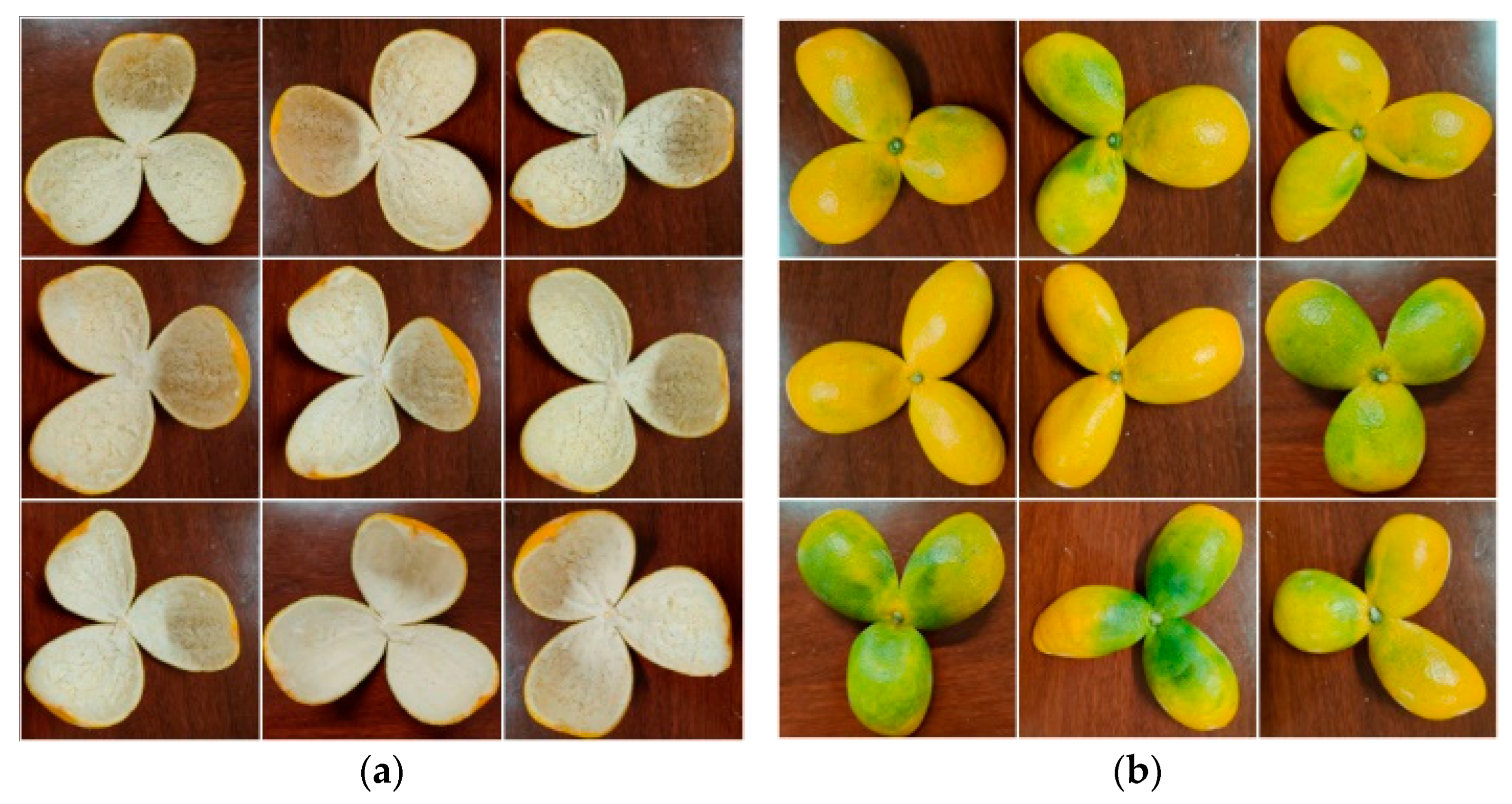
In this study, images reflecting mass loss and morphological changes of tangerine peel across different drying stages were systematically collected under controlled temperature, wind speed, and standardized illumination conditions. A spatiotemporal correlation analysis between drying kinetic parameters (temperature, wind speed) and apparent features (e.g., texture, contour) was conducted, and a multimodal dataset for tangerine peel drying kinetics was established.

3.2. Tangerine Peel Image Segmentation

This study adopted VGG-UNet as the baseline model for image segmentation of tangerine peel, selected for its architectural adaptability to the complex surface morphology of tangerine peel. The surface of the tangerine peel exhibits multi-scale textural structures (e.g., dense oil glands), irregular edges (wrinkles and speckles), and light-sensitive color gradients. These features present challenges for local feature sensitivity and the retention of spatial information. The hybrid architecture of VGG-UNet effectively addresses these issues through its design [16].

The pre-trained VGG16 encoder comprises 13 layers of 3 × 3 convolution kernels, which progressively extract features from low-level textures (e.g., oil gland units) to high-level semantic structures. The decoder employs an upsampling path that merges features from different encoder levels via skip connections, effectively restoring blurred edge regions caused by surface wrinkles. Furthermore, the UNet framework offers excellent segmentation performance and fast training convergence, especially with small datasets.

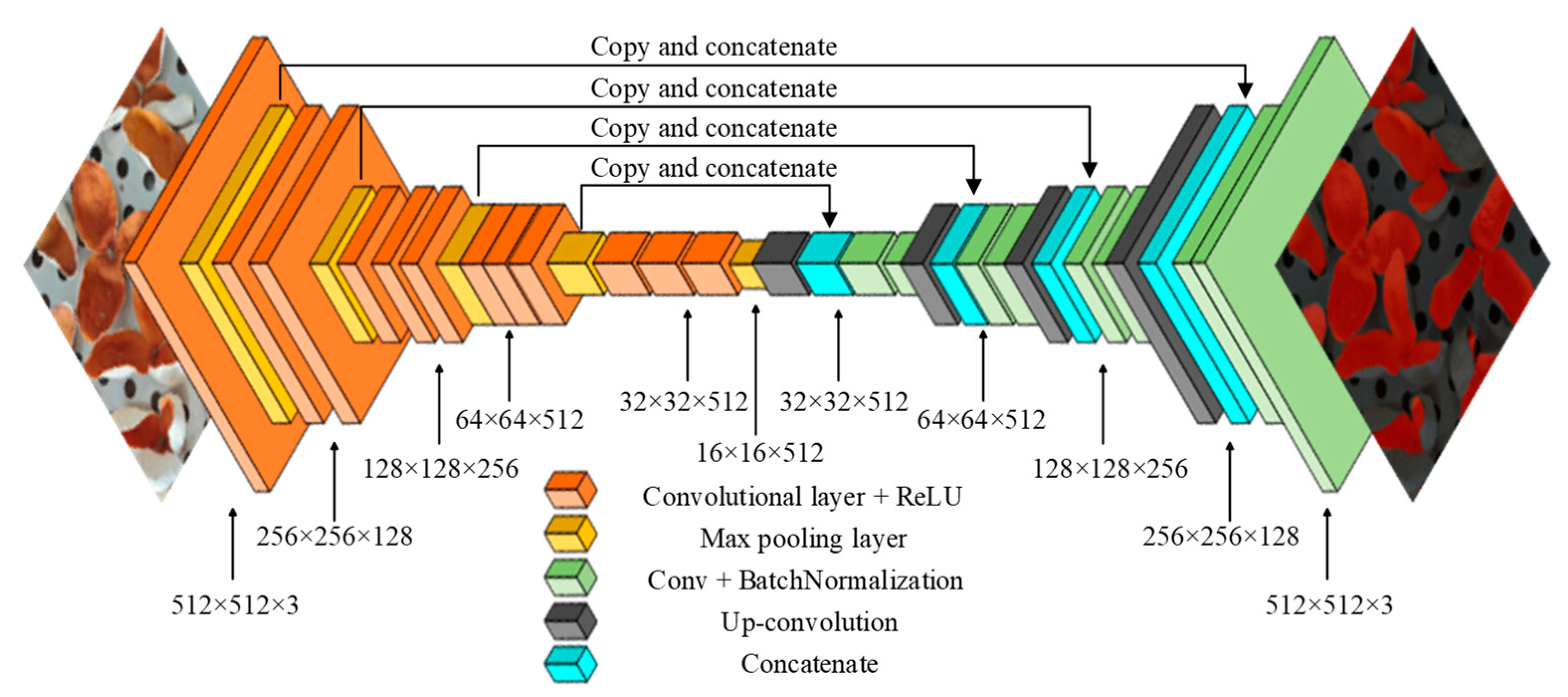
Accordingly, this study utilizes the VGG-UNet network as the foundational model for the segmentation task, as illustrated in Figure 6.

The parameter changes of VGG-UNet are shown in Figure 5. The initial 13 convolutional layers from VGG16 were used as the feature extraction module. Each layer employs a 3 × 3 kernel, and the number of filters is set to 64, 128, 256, and 512, respectively. The ReLU function is used as the activation function. The encoder performs downsampling via convolution and pooling, compressing the image from 512 × 512 × 3 to 32 × 32 × 512 across four downsampling steps. This effectively compresses the tangerine peel’s features. The decoder reconstructs the segmented image through continuous upsampling and convolution, restoring the output size to 512 × 512. The VGG16-UNet semantic segmentation model performs four-stage feature fusion, where encoder feature maps are merged with corresponding decoder feature maps through skip connections. This facilitates the fusion of low-level spatial and high-level semantic information, enabling accurate tangerine peel segmentation.

3.3. Tangerine Peel Image Feature Extraction

To comprehensively characterize the shape, color, and texture of the segmented tangerine peel regions, a multi-dimensional feature extraction approach was adopted. High-quality input data for subsequent modeling and analysis were obtained through precise contour detection and color space analysis.

3.3.1. Color Feature

Color features serve as an important basis for differentiating tangerine peel. In this study, statistical color descriptors were extracted from both RGB and $L*a*b*$ color spaces, including the mean and standard deviation [14]. By integrating features from both color spaces, the model benefits from the high sensitivity of RGB to absolute color changes and the perceptual uniformity and illumination invariance of $L*a*b*$.

Define image $I\left(x,y,c\right)$ as a three-channel matrix, where $c\in \left\{R,G,B\right\}$. For each channel, calculate the mean ${\mu }_c$ and standard deviation ${\sigma }_c$:

$${\mu }_c={\displaystyle \frac{1}{N}}{\displaystyle \sum _{x=1}^H{\displaystyle \sum _{y=1}^{W}I\left(x,y,c\right)}}$$

(7)

$${\sigma }_c=\sqrt{{\displaystyle \frac{1}{N}}{\displaystyle \sum _{x=1}^H{\displaystyle \sum _{y=1}^W{(I(x,y,c)-{\mu }_c)}^2}}}$$

(8)

Among them, $N=H\times W$ represents the total number of pixels, H and W are the height and width of the image.

The RGB image is converted to the $L*a*b*$ color space, and the above mean and standard deviation calculation method is repeated to obtain the mean ${\mu }_{L,a,b}$ and standard deviation ${\sigma }_{L,a,b}$ of the $L\backslash *, a\backslash *, b\backslash *$ three channels. The normalized red, green, and blue index $r, g, b$ was calculated to represent the color distribution ratio.

3.3.2. Contour Feature

Contour features of the segmented regions were extracted from binary images using the OpenCV contour detection algorithm. The calculated features include perimeter (L), area (S), circularity (Cir), and compactness (Com). The specific equations are as follows:

$$Cir={\displaystyle \frac{4\pi S}{L^2}}$$

(9)

$$Com={\displaystyle \frac{L^2}{S}}$$

(10)

where L is the perimeter and S is the area. A circularity value of 1 indicates a perfect circle; lower values signify increasing shape irregularity. Similarly, lower compactness values suggest more compact object shapes.

3.3.3. Texture Feature

The degree of shrinkage experienced by the tangerine peel during drying is quantified using texture features derived from the gray-level co-occurrence matrix (GLCM). Six texture metrics are extracted: mean (Mean), contrast (Con), angular second moment (ASM), correlation (Corr), entropy (Entr), and inverse difference moment (IDM).

3.4. KAN-BiLSTM Moisture Ratio Prediction Model

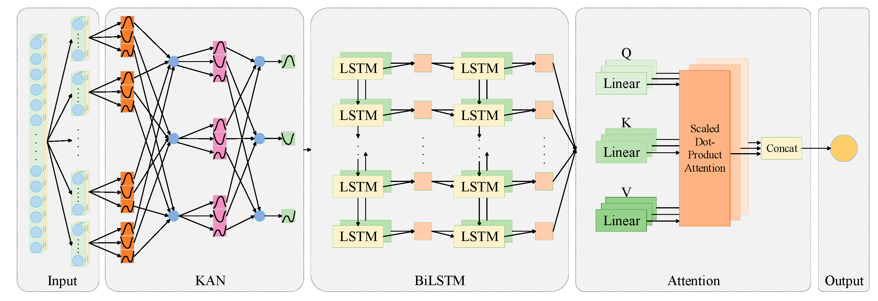
In this study, a novel KAN-BiLSTM moisture ratio prediction model was constructed by integrating the KAN layer and the MHA mechanism into a bidirectional long short-term memory (BiLSTM) framework. The architecture of the proposed model comprises five main components: Input, KAN, BiLSTM, MHA, and Output layers.

3.4.1. KAN (Kolmogorov-Arnold Networks)

The theoretical foundation of the KAN is based on the Kolmogorov–Arnold representation theorem, which states that any multivariate, continuous, and smooth function defined over a bounded domain can be decomposed into a finite sum of univariate continuous functions [15]. Building on this principle, KAN parameterizes the learning of high-dimensional functions as a process of adaptively combining univariate basis functions using polynomial transformations [25]. The structural innovation of KAN lies in its ability to learn univariate activation functions at the network’s edge, introducing nonlinear mechanisms that enable effective modeling of complex functional relationships. This substantially enhances the network’s capacity to represent temporal features.

Theoretical analyses and empirical studies have demonstrated that KAN exhibits superior neural scaling properties compared to conventional architectures. This advantage arises primarily from two factors: (1) the replacement of parameterized weight matrices with analytically defined univariate basis functions that can be individually fine-tuned, and (2) the relaxation of constraints imposed by fixed activation functions, allowing for dynamic optimization of activation patterns.

Formally, for an n-dimensional input–output system, KAN can be modeled as a function matrix that maps an n-dimensional input to an n-dimensional output [20]. A single KAN layer, as illustrated in Figure 7, can be expressed using Equation (11) and the matrix form in Equation (12) [19,26]:

$$x_{l+1,j}={\displaystyle \sum _{i=1}^{n_l}{\tilde{x}}_{l,j,i}}={\displaystyle \sum _{i=1}^{n_l}{\varphi }_{l,j,i}}(x_{l,j}), j=1,\dots ,n_{l+1}$$

(11)

$$X_{l+1}=\left(\begin{array}{ccc}{\varphi }_{l,1,1}(\cdot )& \dots & {\varphi }_{l,1,n_l}(\cdot )\\ {\varphi }_{l,2,1}(\cdot )& \dots & {\varphi }_{l,2,n_l}(\cdot )\\ ⋮& ⋮& ⋮\\ {\varphi }_{l,n_{l+1},1}(\cdot )& \dots & {\varphi }_{l,n_{l+1},n_l}(\cdot )\end{array}\right)X_l$$

(12)

Among them, $(l,i)$ represents the $i$th neuron in the $l$ layer, and $x_{l,i}$ represents the activation value of the $(l,i)$ layer neurons. The pre-activation value of ${\varphi }_{l,j,i}$ was $x_{l,i}$, and the post-activation value of ${\varphi }_{l,j,i}$ was ${\tilde{x}}_{l,j,i}\equiv {\varphi }_{l,j,i}\left(x_{l,i}\right)$. KAN is generally composed of multiple KAN layers. When the input vector $X$ is given, the output of KAN is [4]:

$$KAN(X)=({\varphi }_{L-1}\circ {\varphi }_{L-2}\circ \dots \circ {\varphi }_1\circ {\varphi }_0)X$$

(13)

In this equation, the intermediate matrix corresponds to the function matrix of the l-th KAN layer.

In this study, the KAN layer functions as the feature extraction module within the KAN-BiLSTM model. By embedding KAN into the architecture, the impact on training outcomes was analyzed to evaluate its effectiveness in enhancing prediction performance.

3.4.2. KAN-BiLSTM

In this study, an enhanced prediction model, KAN-BiLSTM, is proposed. The overall architecture of the model is illustrated in Figure 7. The input layer receives tangerine peel drying data and preprocesses it into a format compatible with the KAN layer. The KAN layer performs nonlinear transformations on the input features, thereby decoupling feature learning from temporal modeling. This enhances the model’s ability to express complex input characteristics. The transformed features are then passed to the BiLSTM module for temporal sequence modeling. The BiLSTM unit employs a bidirectional gating mechanism—consisting of a forget gate, input gate, and output gate [27]—to simultaneously capture both forward and backward temporal dependencies present in the drying process. The first BiLSTM layer captures primary temporal features, and its output is passed through a fully connected layer before entering the second BiLSTM layer, which extracts higher-level temporal dependencies. Subsequently, the output from the BiLSTM is fed into an MHA module. This mechanism dynamically assigns weights to different time steps and features, enabling the model to focus on critical moments and subtle moisture variations, thereby improving prediction accuracy.

As shown in Figure 7, the multi-head attention mechanism achieves this goal by mapping the input sequence to a query (Q), key (K), and value (V) vector, respectively. Subsequently, it employs an attention-scoring function to compute the attentional weights of each position relative to the others, effectively capturing long-range dependencies across the input sequence. The outputs of multiple attention heads are concatenated to form a comprehensive representation. Finally, the output layer produces the model’s final prediction results. The MHA mechanism computes the attention output as follows:

$$Attention(Q,K,V)=softmax\left({\displaystyle \frac{Q{K}^T}{\sqrt{d_k}}}\right)V$$

(14)

where Q, K, and V represent the query, key, and value matrices, respectively, and d_k is the dimension of the key vectors. In the multi-head configuration, the attention mechanism is computed in parallel across multiple heads:

$$MultiHead(Q,K,V)=Concat(hea{d}_1,\dots ,hea{d}_h)W^O$$

(15)

where each attention head is defined as:

$$hea{d}_i=Attention(Q{W}_i^Q,K{W}_i^K,V{W}_i^V)$$

(16)

Here, $W_i^Q$, $W_i^K$,$W_i^V$, and $W^O$ are learned parameter matrices. This structure allows the model to attend to information from different representation subspaces, improving its ability to capture temporal dependencies and feature interactions critical to moisture prediction.

The KAN layer uses 32 neurons and cubic spline curve basis functions. This configuration is determined based on the ablation results (

Table 3. Ablation experiments to analyze the effect of different UNITS values on model performance.

Units	RMSE 1	MAE 2	Parameters
16	0.026	0.019	71 K
24	0.034	0.027	78 K
32	0.019	0.014	85 K
40	0.023	0.016	92 K
48	0.018	0.013	99 K

¹ RMSE: root mean square error; ² MAE: mean absolute error.

) and comparison experiments (

Table 4. Performance comparison of different spline orders.

Spline Order	RMSE	Inference Time (ms)	Parameters
2	0.020	9	84 K
3	0.018	10	85 K
4	0.018	16	86 K
5	0.019	16	87 K

), considering both the model’s expressiveness and its computational efficiency, which is measured in terms of parameter size and inference time.

Ablation experiments reveal that using fewer neurons leads to a notable decline in model performance. For instance, reducing the neuron count to 16 results in a 36.8% increase in RMSE. Conversely, increasing the number of neurons to 48 slightly improves RMSE by 5.3%, but at the cost of a 16.5% increase in computational complexity. Thus, selecting 32 neurons strikes an optimal balance between predictive accuracy and resource efficiency.

In terms of basis function selection, the comparison experiment (Table 4) demonstrates that the quadratic spline (order 2) results in an 11.1% higher RMSE than the cubic spline. While higher-order splines (order ≥ 4) do not show further RMSE reduction compared to the cubic spline, they significantly increase inference time (by up to 60%) and model parameters (by 2 K). Therefore, cubic spline functions are adopted to ensure a balanced trade-off between model capacity and computational efficiency.

After optimization, the MHA layer is configured with 4 heads and embedding dimension (Dim) = 8, which not only satisfies dimensional consistency but also enhances prediction performance. As shown in

Table 5. Ablation study comparing different MHA configurations.

Heads	Dim 1	RMSE	MAE	Params
2	16	0.031	0.024	85 K
4	8	0.027	0.020	85 K
4	16	0.027	0.020	94 K
8	4	0.033	0.023	85 K

¹ Dim: dimension.

, this configuration achieves RMSE = 0.027 and MAE = 0.0202, outperforming other combinations with no increase in parameter count (85 K). The key design consideration is that Dim = 8 matches the 32-dimensional output of the preceding BiLSTM layer (as 4 heads × 8 dimensions = 32), ensuring compatibility, preventing redundancy, and preserving the integrity of feature representations in attention computation.

Further ablation analysis validates the superiority of this setting. Compared to Heads = 2, Dim = 16 (RMSE = 0.0312, MAE = 0.0242), the proposed Heads = 4, Dim = 8 setting reduces RMSE by 12.8% and MAE by 16.5%, with an identical number of parameters. Although Heads = 4, Dim = 16 yields comparable performance, it incurs a 10.6% increase in parameter count. These findings indicate that the selected configuration achieves an optimal balance among representational capacity, computational efficiency, and dimensional alignment with the upstream features.

3.5. Model Evaluation Indicators

All statistical analyses were conducted using Python (version 3.9), leveraging libraries such as NumPy, SciPy, and scikit-learn. Descriptive statistics, including the mean and standard deviation, were calculated to summarize the central tendency and dispersion of the extracted image features and moisture content data.

The performance of the proposed model was evaluated using the following statistical metrics: coefficient of determination (R²), mean absolute error (MAE), root mean square error (RMSE), mean intersection over union (MIoU), and F1-score. The detailed formulas are shown in Equations (17)–(21) [21]:

$$RMSE=\sqrt{{\displaystyle \frac{1}{N}}{\displaystyle \sum _{k=1}^N{(P_k-R_k)}^2}}$$

(17)

$$MAE={\displaystyle \frac{1}{N}}{\displaystyle \sum _{k=1}^N(\left|R_k-P_k\right|)}$$

(18)

$$R^2=\left\{{\displaystyle \frac{{\displaystyle \sum _{k=1}^N(P_k-\overline{P})(R_k-\overline{R})}}{\sqrt{{(P_k-\overline{P})}^2}\sqrt{{(R_k-\overline{R})}^2}}}\right\}$$

(19)

$$\mathrm{MIoU}={\displaystyle \frac{1}{\mathrm{m}}}{\displaystyle \sum _{l=1}^{\mathrm{m}}\frac{TP}{TP+FP+FN}}$$

(20)

$$F1-score={\displaystyle \frac{2\cdot TP}{2\cdot TP+FP+FN}}$$

(21)

In the above formulas, $R_k$ is the actual moisture ratio of group k data; $P_k$ is the predicted moisture ratio of group k data; $\overline{R}$ is the average value of $R_k$; $\overline{P}$ is the average value of $P_k$; and N is the number of samples. TP indicates that the sample is predicted to belong to the positive category, and its real label is also shown as a positive category; FN indicates that the sample is incorrectly predicted as a reverse category, and its true label is a positive category; FP means that the sample is incorrectly predicted as a positive category, while its true label is a reverse category; TN indicates that the sample is correctly identified as a counterexample and is consistent with its true label; m is the category; $l$ represents the true value. Furthermore, a 95% confidence interval (CI) analysis was performed on the MIoU values to evaluate the statistical significance of differences across model configurations.

3.6. Experimental Workflow

The prediction method of tangerine peel dry moisture ratio based on KAN-BiLSTM and multimodal feature fusion is summarized as Algorithm 1.

Algorithm 1: Prediction method of tangerine peel drying moisture ratio based on KAN-BiLSTM and multimodal feature fusion

Input:        Tangerine peel morphological evolution image data;        Moisture loss data of tangerine peel;        Spatial position data of drying oven; Output:        Segmentation image of tangerine peel;        Predicted moisture ratio of tangerine peel; For each t ranging from 1 to the last tangerine peel image N. 1. Preprocess the image: standardization and resizing; 2. Perform encoder-based feature extraction (refer to the left half of Figure 6); 3. Perform pixel-level segmentation using the decoder (refer to the right half of Figure 6); 4. Extract the red channel range to generate a binary mask of the tangerine peel area; 5. Integrate the segmented image with the actual moisture data and spatial position data to construct a multimodal dataset for tangerine peel drying; 6. Use the KAN layer as the feature extraction layer, providing input to BiLSTM (see Figure 7); 7. Construct the KAN-BiLSTM regression model (see Figure 7); 8. Predict the moisture ratio for the target image.

End for

4. Results and Analysis

4.1. Dataset

4.1.1. Tangerine Peel Moisture Loss Dataset

A total of 480 groups of original moisture loss data were acquired from the tangerine peel drying tests described in Section 2.3.3, with each group accompanied by corresponding images. All experiments were conducted under strictly controlled environmental conditions to ensure the repeatability and reliability of the data. During testing, moisture variations for each sample group were measured using a high-precision electronic analytical balance (Leqi CZ3003, accuracy 0.001 g) and synchronized with image data to facilitate subsequent image feature extraction and deep learning analysis.

To ensure data standardization, preprocessing steps including outlier detection, data smoothing, and normalization were applied. Each record included test time (min), tangerine peel mass (g), dry basis moisture content (g/g), moisture ratio (MR), and test environmental parameters (temperature, wind speed, humidity, and light). This comprehensive dataset served as the basis for subsequent deep learning-based model optimization for real-time moisture content prediction during tangerine peel drying.

4.1.2. Spatial Location Data Set

Based on the spatial location feature extraction approach detailed in Section 3.1, three groups of original spatial location data were obtained, with each group comprising 26,000 data points. Finite element analysis (FEA) was employed to model and analyze the temperature field distribution inside the drying chamber. This analysis refined the temperature region division and validated the rationality of the hierarchical clustering results.

The spatial location dataset of the tangerine peel drying temperature field consists of three components as follows:

• Spatial coordinate information (x, y, z): The three-dimensional positions of the temperature field in the drying chamber were extracted at a resolution of 5 mm, yielding a total of 26,000 points;
• Temperature field values (T): The temperature value (in Kelvin) associated with each spatial point;
• Regional temperature labels: The temperature field data were segmented into six regions via hierarchical clustering, and each data point was assigned a corresponding regional label.

This dataset was utilized to train a deep learning model for prediction, enabling moisture ratio analysis based on regional temperature characteristics.

4.1.3. Semantic Segmentation Image Data Set

For the semantic segmentation task, a total of 1325 original experimental images were acquired during the tangerine peel drying tests, from which 1680 real tangerine peel drying images were obtained after screening and enhancement. The primary objective was to achieve accurate segmentation of the tangerine peel. The image labels were categorized into tangerine peel and background and were subsequently divided into training and test sets at a 9:1 ratio. The training set comprised 1512 images, while the test set contained 168 images, ensuring a balanced distribution for effective model training and evaluation. The high quality and precision of the image annotations provide a reliable basis for subsequent experiments.

4.2. Experimental Environment

The experiments were conducted on a Windows 11 operating system using an Intel^® CORE™ i9-13900K CPU. For deep learning computations, a dual GeForce RTX 4080 graphics card configuration with 32 GB of memory was employed. The deep learning framework used for model development was PyTorch (1.3.0).

4.3. Regionalization Results

In ANSYS Fluent, numerical data from the temperature cloud map were extracted, including spatial coordinates (x, y, z) and corresponding temperature values. At each specified height, a set of 26,000 data points was obtained. The temperature values were used as the primary feature for clustering analysis. An example of such data is presented in

Table 6. Numerical data of temperature cloud map.

Material Board Height	Position and Temperature on Different Material Plates
	X [m]	Z [m]	Temperature [K]
Y = 0.8	−1.26 × 10−1	−2.41 × 10−1	2.97 × 102
	−1.25 × 10−1	−2.42 × 10−1	2.97 × 102
	−1.26 × 10−1	−2.42 × 10−1	2.97 × 102
Y = 0.535	−1.12 × 10−2	−2.50 × 10−1	2.88 × 102
	−1.12 × 10−2	−2.50 × 10−1	2.88 × 102
	−1.12 × 10−2	−2.50 × 10−1	2.88 × 102
Y = 0.35	1.40 × 10−1	−2.50 × 10−1	2.88 × 102
	1.43 × 10−1	−2.50 × 10−1	2.88 × 102
	1.42 × 10−1	−2.48 × 10−1	2.89 × 102

.

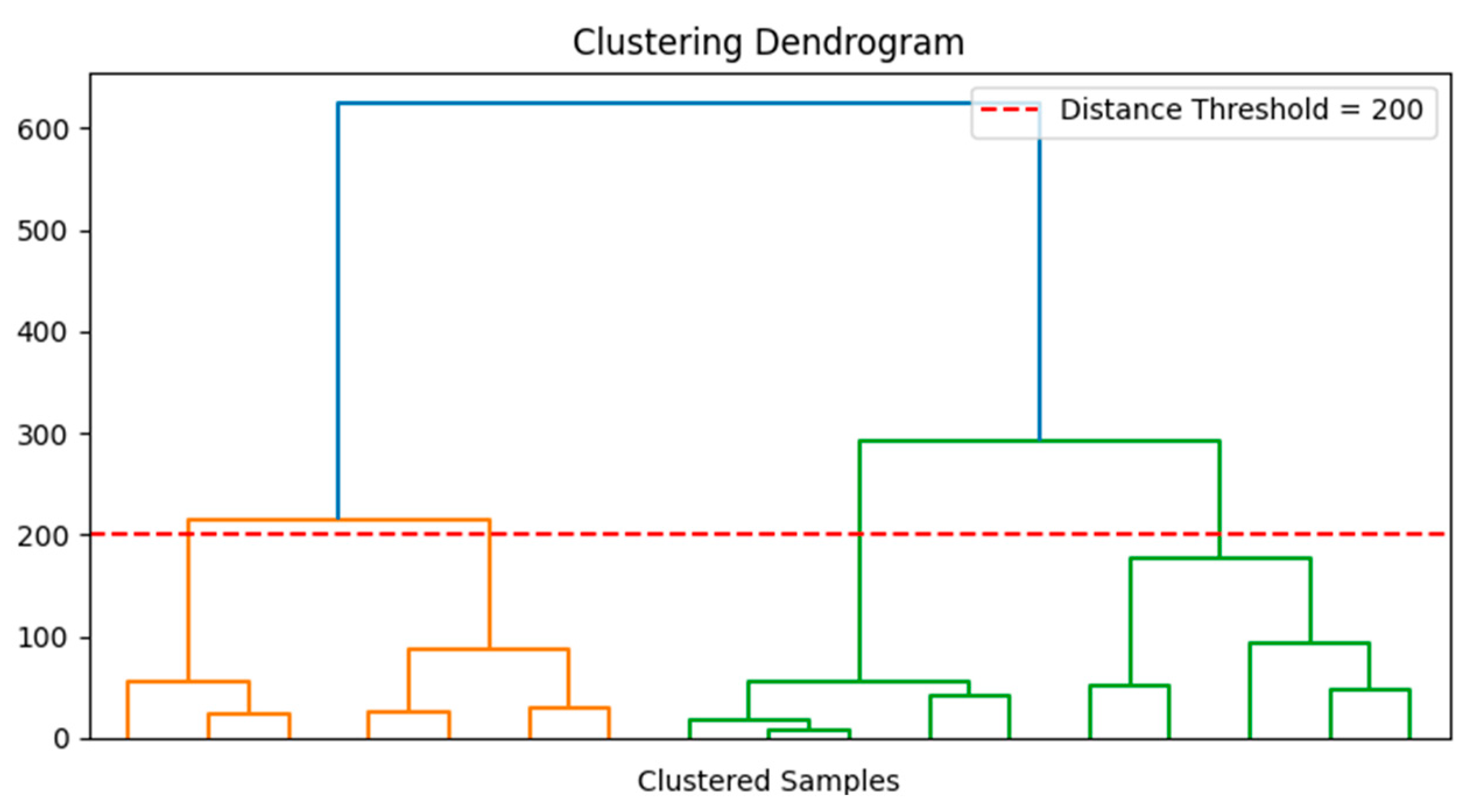
The temperature variations observed in the cloud map are closely related to spatial position. The Euclidean distance was employed to quantify the linear distance between data points, thereby facilitating the identification of the temperature distribution. Accordingly, the Euclidean distance was chosen as the metric for temperature segmentation, with a threshold set to 200. The resulting clustering is illustrated in Figure 8.

The clustering dendrogram illustrates the sample grouping based on Euclidean distances. A distance threshold of 200 (red dashed line) was applied to truncate the dendrogram, resulting in the identification of three distinct clusters. But, in the actual material board, the same category was distributed on both sides of the center. So, we divided the material board into six regions; you can divide the temperature region on the material board, the results of the division shown in Figure 9 and Figure 10.

The results indicate that the temperature fields in the upper, middle, and lower layers exhibited pronounced gradient distributions, with the upper layer registering relatively higher temperatures. Areas near the air inlet displayed elevated temperatures and steep gradients due to the influence of wind speed. Notably, the regions of local temperature fluctuation corresponded closely with the hierarchical clustering divisions. Therefore, the extracted spatial location features, combined with image features, were integrated into the final feature set used as input for the prediction model.

4.4. VGG-UNet Model Evaluation

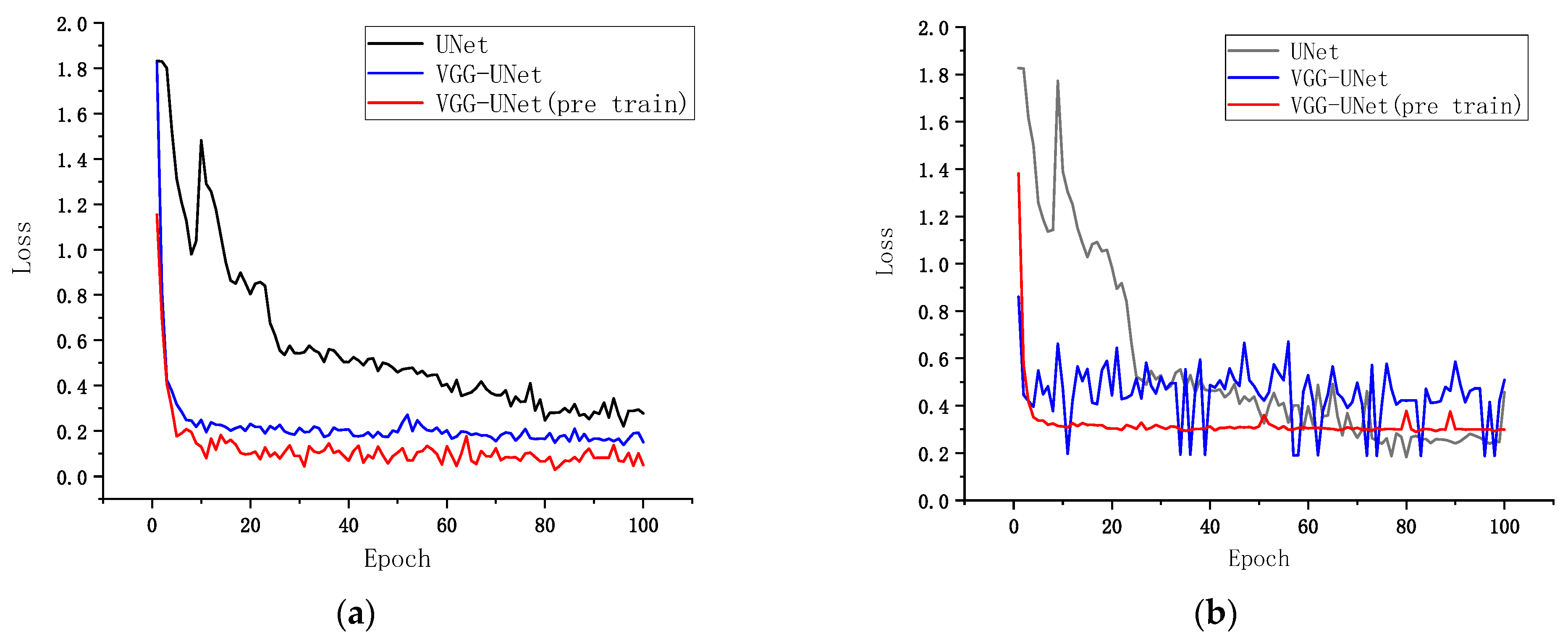
This section compares the performance of U-Net, VGG-UNet, and pre-trained VGG-UNet in the tangerine peel image segmentation task through systematic experiments, with a particular focus on training dynamics and loss convergence characteristics. Prior to model training, all input images were resized to a fixed resolution of 512 × 512 pixels to ensure consistency in input dimensions. All models were trained for 100 epochs using the same hyperparameters (initial learning rate = 0.0001 with the Adam optimizer) on a dataset comprising 1680 high-resolution citrus epidermis images (1344 for training and 336 for validation). The evaluation results in terms of MIoU and loss are presented in

Table 7. Performance analysis of different semantic segmentation models.

Model	MIoU 1 (%)	F1 2	Loss
UNet	84.17 (95%CI 3: 52.892, 73.231)	0.914	0.22
VGG-UNet	80.54 (95%CI: 79.862, 80.450)	0.892	0.17
VGG-UNet (pre-train)	93.58 (95%CI: 89.482, 90.069)	0.967	0.13

¹ MIoU: mean intersection over union; ² F1: F1-score; ³ CI: confidence interval.

.

Figure 11a,b illustrate the convergence rate and stability during training and validation, respectively. Notably, the pre-trained VGG-UNet demonstrates a significantly superior initialization and feature representation capability. Its initial loss at epoch 1 was 1.15, which is approximately 67% and 68% lower than that of the randomly initialized VGG-UNet (1.82) and basic U-Net (1.83), respectively (see Figure 11). Moreover, the MIoU of the pre-trained VGG-UNet was 93.58%, exceeding that of the randomly initialized VGG-UNet (80.54%) and basic U-Net (84.17%) by 13.04 and 9.41 percentage points, respectively (see Figure 12). These results indicate that the use of pre-trained weights effectively alleviates the cold start problem, particularly by capturing general texture features in the shallow convolutional layers. To assess the robustness of the models, we further report the 95% confidence intervals (CI) of MIoU across repeated runs. The pre-trained VGG-UNet showed a narrow CI of [89.482%, 90.069%], indicating high reliability and stability. In contrast, the randomly initialized VGG-UNet had a wider CI of [79.862%, 80.450%], and the basic U-Net showed the lowest robustness with a CI of [52.892%, 73.231%]. We computed the F1-score as a pixel-level performance indicator. As shown in Table 7, the pre-trained VGG-UNet achieved the highest MIoU of 93.58% and a corresponding F1-score of 0.967, significantly outperforming both the basic UNet (F1 = 0.914) and randomly initialized VGG-UNet (F1 = 0.892). These findings underscore the advantage of pre-trained feature extractors in improving both accuracy and consistency of the segmentation performance.

Furthermore, the loss curve of the pre-trained model converged the fastest, reaching a stable plateau at epoch 15 with a loss of 0.15, whereas the randomly initialized VGG-UNet and U-Net only attained stability at epochs 35 and 80, with final loss values of 0.17 and 0.22, respectively. Additional analysis suggests that the parameter space of the pre-trained encoder is closer to an optimal solution.

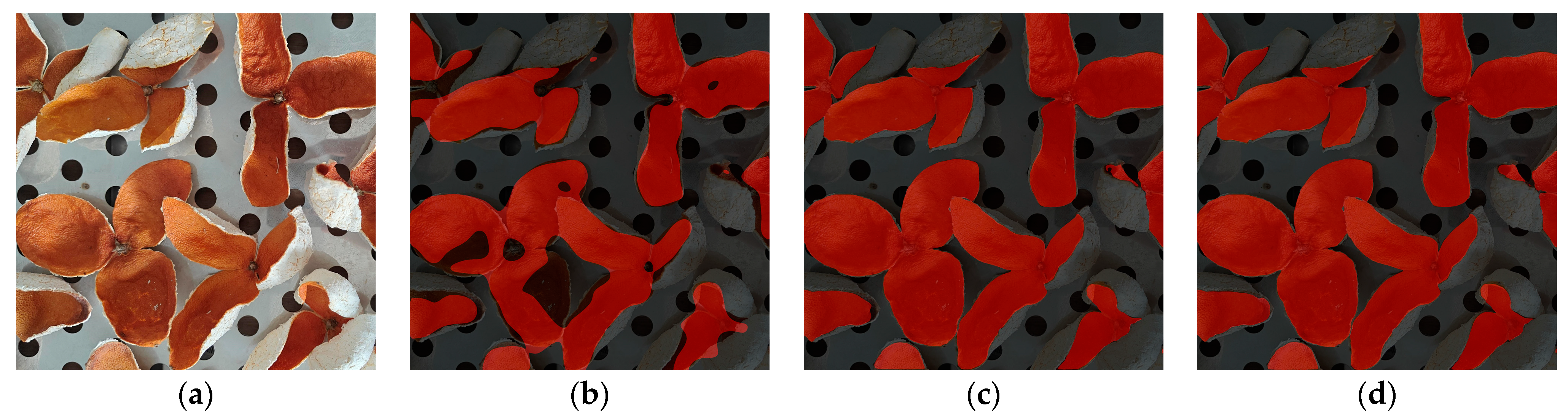
To further validate the segmentation performance of the VGG16-UNet model, tangerine peel images from the test set were segmented and visually compared, as shown in Figure 13. Overall, despite the complex background, the VGG16-UNet model achieved high consistency in multi-target measurements.

In particular, the segmentation accuracy in the tangerine peel–background transition region was markedly superior to that of the other models (see Figure 13). The visualization in Figure 13d demonstrates that the pre-trained model effectively suppressed the edge fragmentation caused by wrinkle shadows, with segmentation contours that closely match the manual ground truth. This performance advantage is attributed to the multi-directional edge filtering capability provided by the VGG16 pre-training, which enhances the model’s ability to accurately characterize irregular boundaries.

In summary, the pre-trained VGG-UNet outperforms the benchmark models in terms of loss convergence speed, fine-grained feature modeling, and generalization capability through the transfer learning of encoder weights. This robust performance renders it an efficient solution for tangerine peel segmentation, and thus it is adopted as the segmentation model in this study.

4.5. KAN-BiLSTM Model Evaluation

Five models—RNN, GRU, LSTM, BiLSTM, and KAN-BiLSTM—were employed to predict moisture and to compare their performance. Prior to training, the data were normalized to a range of 0 to 1 to optimize the neural network’s performance. The dataset was split into training and test sets at a ratio of 70:30, with 30% data further reserved for model validation. The hyperparameter settings for each model are presented in

Table 8. Hyperparameters of different models.

Hyperparameter	RNN	GRU	LSTM	BiLSTM	KAN-BiLSTM
Input	19	19	19	19	19
Epochs	50	30	20	15	10
Batch size	16	16	16	16	32
Loss function	MSE	MSE	MSE	MSE	MSE
Optimizer	Adam	Adam	Adam	Adam	Adam

.

Table 9. Accuracy metrics of various models on the moisture sequence test dataset.

Model	Test
	Region	RMSE	MAE	R2 1
RNN		0.1532	0.0971	0.7285
	√	0.1141	0.0777	0.8495
GRU		0.1350	0.0954	0.7893
	√	0.1207	0.0794	0.8315
LSTM		0.1245	0.0744	0.8208
	√	0.1210	0.0766	0.8306
BiLSTM		0.1043	0.0673	0.8543
	√	0.0907	0.476	0.9049
KAN-BiLSTM		0.0482	0.0352	0.9731
	√	0.0283	0.0240	0.9908

¹ R²: coefficient of determination.

summarizes the accuracy metrics of various models on the moisture sequence test dataset. The results demonstrate that the vanilla RNN yielded an RMSE of 0.1023, an MAE of 0.0687, and an R² of 0.8791, with a relatively long runtime and low efficiency. While GRU significantly improved training speed, the improvements in RMSE, MAE, and R² were modest. Overall, the deep learning models equipped with memory mechanisms exhibited markedly superior prediction accuracy. In particular, the BiLSTM model achieved the best performance, with the RMSE decreasing from 0.1023 (RNN) to 0.0679, the MAE reaching a minimum of 0.0404, and the R² rising to 0.9452. Table 9 also compares the performance of overall and sub-regional predictions within the same model, revealing that sub-regional prediction further enhances moisture content estimation. The incorporation of regional data significantly improves prediction accuracy, demonstrating a positive impact on moisture content forecasting.

Figure 14 compares the actual values and predictions for test data using the four architectures (RNN, GRU, LSTM, and BiLSTM), with and without regional data. Each comparison diagram displays seven change curves that start simultaneously with the same initial moisture ratio. Among these, the red curves represent the true test data, while the blue curves correspond to the predicted values obtained from the model.

The results indicate that the RNN-based model was less effective for long sequence-dependent tasks, with significant errors observed during periods of minimal moisture change. Models such as GRU and LSTM, which incorporate gating and memory mechanisms, better capture the dependence of moisture ratio on additional features, though some discrepancies remain during the critical period of weak moisture variation. The BiLSTM model, leveraging bidirectional processing, more comprehensively interprets the input data. For example, Figure 14d,h illustrate that incorporating regional data results in predictions that closely align with actual values, especially during phases of subtle moisture change, thereby confirming the beneficial impact of regional data on moisture content prediction.

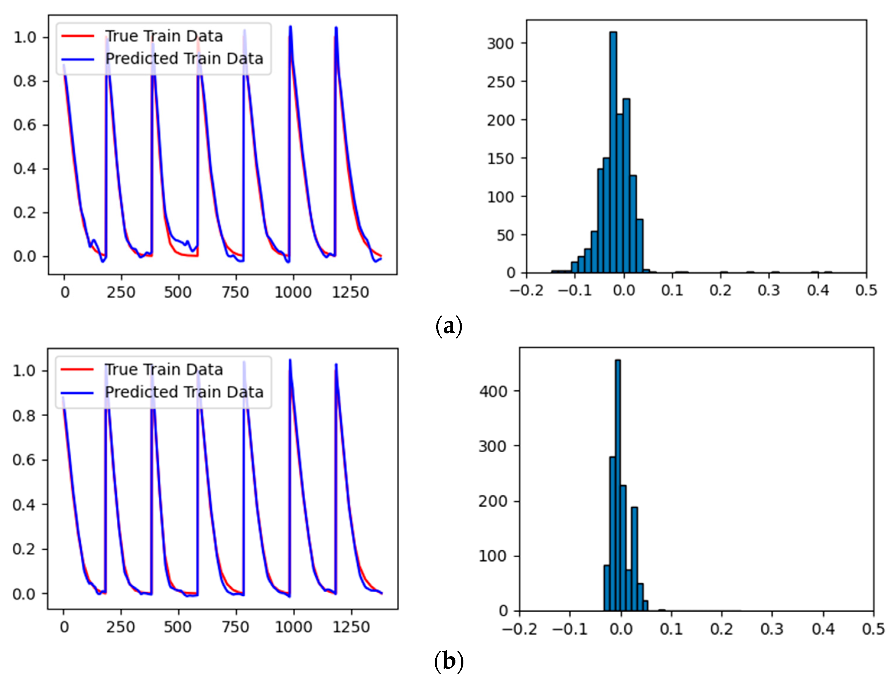
Figure 15 illustrates the error probability distribution curves for the different models. These curves indicate that the BiLSTM model exhibits superior performance compared to the other architectures, as its error distribution is highly concentrated around zero. This concentration implies that the BiLSTM model delivers exceptionally reliable and accurate moisture content predictions throughout the drying process. Consequently, BiLSTM was chosen as the foundational structure for moisture prediction. In the proposed architecture, a KAN layer serves as the feature extraction module supplying input to the BiLSTM, and an MHA mechanism is incorporated between the BiLSTM and the fully connected layers. Ultimately, these components form the final KAN-BiLSTM model.

Figure 16 illustrates the data comparison and error distribution of the KAN-BiLSTM model. Compared with the basic BiLSTM structure, the KAN-BiLSTM model shows improved performance in capturing subtle variations in moisture content, with only minor deviations from the actual drying curve. Notably, in the moisture ratio range from 0.2 to 0—which is typically challenging to model accurately—the nonlinear prediction capability of the model is significantly enhanced.

The experimental results demonstrate that the KAN-BiLSTM model significantly outperformed benchmark models in terms of nonlinear prediction ability; its RMSE, MAE, and R² metrics all surpassed those of the competitors. Consequently, the KAN-BiLSTM model was adopted as the efficient solution for predicting the tangerine peel moisture ratio.

4.6. Moisture Ratio Prediction Experimental Results

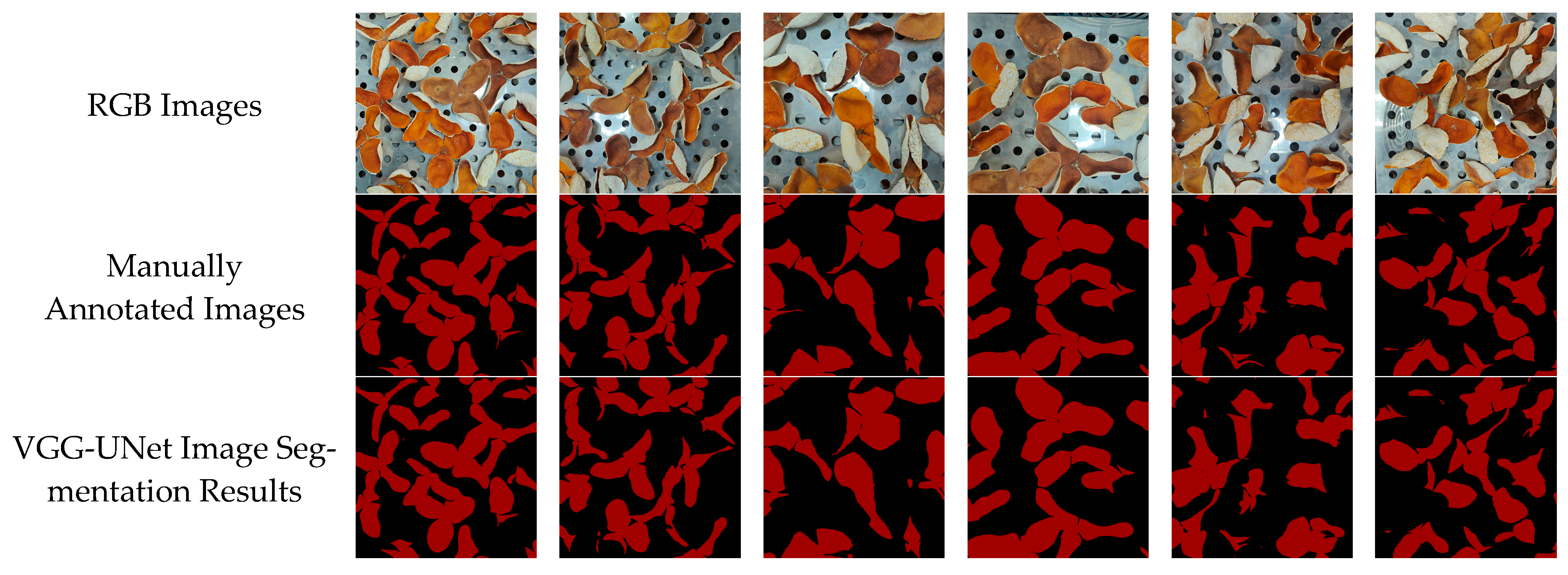
In order to evaluate the segmentation model’s performance, this study compares manually annotated images of real tangerine peel with the VGG-UNet segmentation outputs to obtain an accurate depiction of the morphological evolution. For clarity, segmentation results from six representative images are displayed in Figure 17. Overall, the VGG-UNet segmentation model exhibited a high degree of consistency between the multi-target segmentation results and the corresponding manually annotated images.

Following semantic segmentation to extract the tangerine peel area, the moisture ratio is predicted to yield a real-time estimation of moisture content. The actual moisture ratio is then determined from the measured moisture loss at various drying stages. To assess the prediction model’s performance, the predicted moisture values were compared with the measured values. Relevant data are presented in Figure 17 and

Table 10. Accuracy test results of the KAN-BiLSTM prediction model.

Time	Moisture Ratio/%		Error/%	Relative Error/%
	Predicted Value/%	True Value/%
a	78.4	77.6	0.8	1.03
b	62.3	61.8	0.5	0.81
c	51.6	52.5	0.9	1.71
d	38.4	38.2	0.2	0.52
e	10.5	10.9	0.4	3.67

.

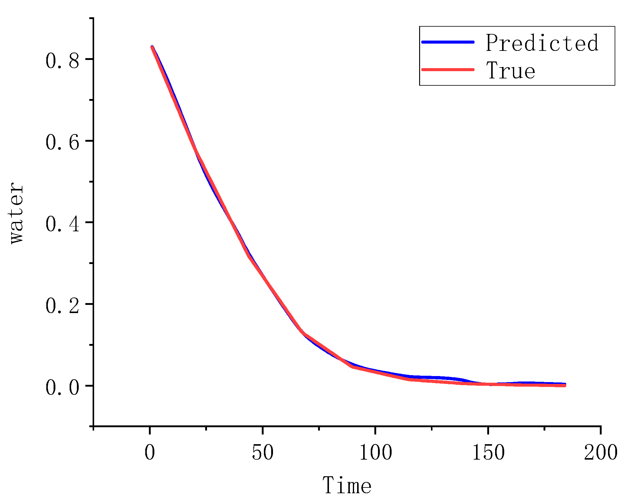
Analysis of Figure 18 reveals that the predicted and measured moisture ratio curves are closely fitted, with a determination coefficient (R²) of 0.998. This high R² value indicates that the model reliably captures the overall drying process of tangerine peel, providing a robust reference for moisture ratio prediction. Furthermore, as illustrated in Table 10, the error in determining the moisture ratio during the heat pump drying process is below 1%. Importantly, regardless of whether the predicted moisture ratio is slightly overestimated or underestimated, the relative error remains within 4%, thereby meeting practical production requirements.

5. Discussion

In this study, a high-precision prediction model for tangerine peel moisture ratio was developed through multimodal data fusion and deep learning techniques, yielding promising results in controlled laboratory settings. However, for real-world deployment and industrial-scale application, several technical and practical aspects warrant further discussion.

Although the model achieved strong predictive performance, we observed that the prediction errors were slightly higher at the initial and final stages of drying—corresponding to high and low moisture values, respectively. These deviations are mainly attributed to rapid morphological changes in the early drying phase and lower contrast or deformation in the late stage, which affect the extraction of visual and spatial features. Future refinements may include temporal segmentation strategies or dynamic feature recalibration to address such transitions. Compared to traditional single-modal models, such as LSTM or CNN-based methods using only mass loss or image features, the proposed KAN-BiLSTM architecture integrates both image-derived features and simulated airflow data to enhance nonlinear learning and temporal reasoning. Prior studies in food drying, such as those by Sabat and Jia, reported R² values around 0.82–0.88 using conventional LSTM-based models [14,22]. In contrast, our model achieved R² = 0.9908 and MAE = 0.024, highlighting its substantial improvements in accuracy and robustness, particularly in capturing spatial heterogeneity and subtle moisture variations.

The multimodal data fusion strategy successfully overcomes the limitations of single-modal approaches in monitoring drying dynamics. This not only enhances segmentation and prediction accuracy but also provides a scientific basis for parameter optimization and process control in drying equipments. Second, by employing the KAN layer as a feature extraction module, the mapping capacity for high-dimensional nonlinear features is significantly enhanced through adaptive nonlinear activation functions. Coupled with the BiLSTM’s ability to capture bidirectional temporal dependencies and the MHA module’s focus on key time steps and features, the proposed method offers a novel approach for precise control of the drying process for tangerine peel and other agricultural products.

In addition to its technical advantages, the model has promising industrial implications. By enabling accurate and real-time moisture prediction, it may reduce energy consumption by preventing over-drying, minimize labor reliance through non-contact monitoring, and support process automation in heat pump drying systems. Furthermore, this multimodal modeling framework is adaptable to other agricultural products with similar surface-texture dynamics, demonstrating good scalability. The ability to monitor drying conditions visually and spatially provides a foundation for intelligent drying control.

It should be noted that the current experiments were conducted under a single drying condition (45 °C and 0.5 m/s airflow), which may limit the model’s generalizability to broader scenarios with varying temperature and humidity settings. While the model structure supports expansion to multivariate conditions, further data collection under diverse drying regimes will be required to evaluate its robustness and adaptability. Moreover, the finite element model simplified thermal interactions by merging the tray, material, and rack into a single material layer. This assumption was made to reduce simulation complexity and computational load, especially during mesh generation. However, it may overlook subtle thermal resistance effects at the interface layers, which could impact the fidelity of the simulated spatial features. Future studies should investigate the quantitative effect of this simplification on prediction accuracy. The integration of KAN and MHA inevitably increases model complexity. Future work should explore lightweight deployment versions for embedded systems. Additionally, although the dataset included 432 samples across six drying batches, its scale and diversity remain limited to a controlled laboratory setup. Broader datasets covering different citrus varieties and drying chamber structures will be required to ensure generalizability.

In summary, while this study proposes a novel and effective approach to predicting drying moisture ratio using multimodal data fusion and deep learning, we acknowledge the current limitations related to simulation assumptions, dataset size, and deployment constraints. Addressing these challenges in future work will be essential to extend the model’s utility beyond research environments and establish a reliable, scalable, and automated solution for industrial drying processes.

6. Conclusions

This study proposed a novel moisture ratio prediction method for tangerine peel drying by integrating a KAN-BiLSTM model with multimodal feature fusion. Visual features were extracted via a pre-trained VGG-UNet segmentation model, while spatial location data were derived from finite element analysis of the airflow field inside the drying chamber. These features were fused and used to train the KAN-BiLSTM model, where the KAN layer enhanced nonlinear feature representation and a multi-head attention mechanism captured key temporal dependencies.

The experimental results demonstrate that the pre-trained VGG-UNet model achieved an MIoU of 93.58% in tangerine peel image segmentation, significantly outperforming the untrained model. Moreover, the inclusion of spatial location features improved the R² of the time series prediction model by 0.02 to 0.12. The final KAN-BiLSTM model delivered robust performance, with an MAE of 0.024 and an R² of 0.9908. These results highlight the effectiveness of multimodal fusion in capturing complex spatiotemporal drying dynamics and offer a promising solution for intelligent, non-contact moisture monitoring in agricultural drying processes.