Analyzing and Predicting the Agronomic Effectiveness of Fertilizers Derived from Food Waste Using Data-Driven Models

Abstract

This study evaluates and estimates the agronomic effectiveness of food waste-derived fertilizers by analyzing plant yield and the internal efficiency of nitrogen utilization (IENU) via statistical and machine learning models. A dataset of 448 cases from various food waste treatments gathered from our experiments and the existing literature was analyzed. Plant yield and IENU exhibited substantial variability, averaging 2268 ± 3099 kg/ha and 32.3 ± 92.5 kg N/ha, respectively. Ryegrass dominated (73.77%), followed by unspecified grass (10.76%), oats (4.87%), and lettuce (2.02%). Correlation analysis revealed that decomposition duration positively influenced plant yield and IENU (r = 0.42 and 0.44), while temperature and volatile solids had negative correlations. Machine learning models outperformed linear regression in predicting plant yield and IENU, especially after preprocessing to remove missing values and outliers. Random Forest and Cubist models showed strong generalization with high R² (0.79–0.83) for plant yield, while Cubist predicted IENU well in testing, with RMSE = 3.83 and R² = 0.78. These findings highlight machine learning’s ability to analyze complex datasets, improve agricultural decision-making, and optimize food waste utilization.

1. Introduction

A circular economy approach promotes nutrient recovery from food waste (FW), reducing reliance on mined phosphorus (P) and synthetic nitrogen (N) fertilizers [1]. Despite the environmental impact of mineral fertilizers, many nutrient-rich waste sources remain underutilized. Integrating bio-based fertilizers into agriculture enhances soil quality and promotes sustainable food production [2,3,4,5].

The disposal of FW without recycling leads to the loss of valuable nutrients that could otherwise support agricultural productivity. Globally, FW represents approximately one-third of total food production, amounting to 1.3 billion tons annually [6]. FW’s disposal via landfills and incineration causes severe environmental harm, while recycling focuses on converting FW into valuable chemicals and bioenergy [7,8]. FW can be converted into biofertilizers through composting and anaerobic digestion (AD). Composting produces nutrient-rich organic matter, while AD generates biogas and nutrient-dense digestate, offering a sustainable alternative to synthetic fertilizers [9]. Research has explored FW recycling through AD, thermal hydrolysis, and dehydration to create biofertilizers as substitutes for inorganic fertilizers [4,5,10,11,12]. Biofertilizers often result from fermenting or composting kitchen waste alongside other organic materials [13].

Fertilizers significantly influence plant yield (PY), making accurate predictions essential for agricultural planning and food security. Machine learning (ML) has emerged as a powerful tool for prediction in environmental sciences [14,15,16,17] and, specifically, for optimizing crop yields based on fertilizer use [18,19,20]. For example, Li et al. [18] analyzed 35 years of fertilizer application and grain yield data in China, finding that backpropagation neural networks (BPNN) outperformed other ML models, with an RMSE below 0.12 and R² > 0.80. Wang et al. [19] optimized planting density and fertilizer rates using BPNN and regression methods. Thai et al. [21] applied analysis of variance, linear mixed-effects models, and regression trees to evaluate winter wheat yields under different fertilizer practices. Similarly, Meng et al. [20] demonstrated that Random Forest (RF) and adaptive boosting significantly improved yield predictions (R² = 0.85–0.98).

In addition to PY, the fertilizer value of FW after various treatments was assessed using the internal efficiency of nitrogen utilization (IENU). IENU evaluates how efficiently crops use nitrogen for growth, measuring sustainability and optimization in crop production [22,23]. PY represents the agricultural output harvested per unit area, making it a widely used metric for assessing fertilizer impact on crop performance. Both metrics are crucial for evaluating the effectiveness of FW-based fertilizers and FW mitigation programs. However, while PY is frequently applied in such assessments, IENU has received limited attention in practical applications. To the best of our knowledge, no prior studies have systematically applied ML models to predict FW-driven crop yields incorporating both PY and IENU metrics. A comprehensive literature search was conducted to confirm this gap.

The study aims to achieve three key objectives: first, to develop a comprehensive dataset of fertilizers derived from FW; second, to identify and analyze crop yield data influenced by FW-based fertilizers; and third, to estimate the agronomic effectiveness of these fertilizers using statistical and ML models, particularly through PY and IENU. By addressing these objectives, the research aims to enhance the understanding of how FW-driven fertilizers influence crop productivity and nutrient utilization efficiency, ultimately providing valuable insights to improve waste recycling efforts and optimize agricultural practices.

2. Materials and Methods

2.1. Experiments About Kitchen Waste Recycling as Fertilizer for Plant Growth

2.1.1. In-House Experimental Procedures

The dataset used in our experiments comprises 102 cases, including data from our previous studies [13], and recent experiments [24]. The experimental methods for these data were based on the following methodology.

The preparation of the final fertilizer began with creating a model waste mixture composed of 100 g each of banana, tomato, lettuce, fruit juice, bun, and apple, along with 200 g each of flowers and paper. The ingredients were pre-cut with a knife and ground twice using a meat grinder to form a homogeneous paste. The model waste paste exhibited a total solids (TS) content of 54% and a volatile solids (VS) content of 90% (based on TS).

Various pre-treatment methods were applied before fertilizer production, involving combinations of microbial inoculation, natural decay, sterilization, and fermentation:

• In the first scenario, effective microorganisms (EM) were added directly to the model waste.
• In the second scenario, the waste was left to decay for 12 days before introducing a double dose of EM.
• In the third and fourth scenarios, the waste was sterilized after 12 days; however, only the third scenario included EM addition.
• In the final scenario, the waste was allowed to decay and was sterilized but not inoculated with EM.

After pre-treatment, the waste was pre-dried, pelletized, and dried to produce the final fertilizer.

2.1.2. External Investigations

To supplement our experimental data, we extracted and standardized information from 20 additional published studies (

Table 1. Summary of treatment methods and other conditions of selected studies for this work.

Nr	Treatment	Season	Growth Time (Months)	Plant	References
1	(1) Effective Microbes 1 M Incubation, pelleted; (2) Anaerobically Digested, centrifuged; (3) Anaerobically Digested, centrifuged, dried;	Cold, Warm	1, 2, 3, 4, & 6	Ryegrass	[13]
2	(1) Dried, pelletized; (2) Effective Microbes 1 M Incubation, ground; (3) Effective Microbes ×2 1 M Incubation, ground; (4) Sterilized at 70 °C, dried; (5) Stillage added, Anaerobically Digested, centrifuged; (6) Fish waste, Stillage added, Anaerobically Digested, centrifuged	Warm	1, 1.5, & 2, 3	Ryegrass	[24]
3	FW Compost 340, 680, 1020	Warm	0.5, 1, & 1.5	Lettuce	[25]
4	FW 1.1, 1.2, 1.3; Organic Fraction of MSW 1.1, 1.2, 1.3; FW 1, 2, 3 digested; Organic Fraction of MSW digested	Warm	1, 2, & 5.3	Ryegrass	[26]
5	Green Waste compost in different ratios	NA	2.73, 3.0, 3.63, & 9.37	Oat	[27]
6	Garden Waste compost in different ratios	NA	0.75, 1.5, 3.0, 9, & 13	Ryegrass	[28]
7	Composted municipal solid waste 1.1, 2.1, 2.2	NA	4	Ryegrass and wheat	[29]
8	Green Waste Compost 1, 2	NA	12	Oat	[30]
9	Compost 1.1, 1.2, 2.1, 2.2	NA	NA	Oat grass	[31]
10	Straw + slops compost 1.1, 1.2; Slops compost 1.1, 1.2	NA	NA	Winter wheat	[32]
11	Fertilizer granulate obtained from biogas digestate in different ratios	NA	12, 24, 36, & 48	Grass	[33]
12	Compost 1, 2	NA	1	Corn	[34]
13	100% FW digestate; 10% FWD, 90% fertilizer; 50% FWD, 50% fertilizer	Cold	40	Shoots Kai choy	[35]
14	FW + yard trimmings + paper; FW + wood waste + sawdust	Warm	180	Grass	[36]
15	Mixed DD, LD, and MIN	Warm and Cold	62 & 64	Lactuva sativa	[37]
16	Municipal solid FW compost	Cold	120	Oat	[38]
17	Chemical fertilizer + 100%, 150%, and 300% FW-livestock manure compost	Warm	180	Rice	[39]
18	FW digestate, I, II; FW co-digested with sewage sludge, I and II	Warm	NA	Barley and Oats	[40]
19	Acidulous composting FW	Spring	85, 99 & 100	Potato	[41]
20	Green waste compost	NA	2.73, 3.00, 3.63, & 9.37	Oat	[42]

Notes: Not available (NA); Food waste (FW); Dried digestate sampled from liquid digestate (DD); Liquid digestate (LD); mineral fertilizer (MIN).

). Together, these datasets formed the comprehensive database for modeling purposes.

Table 1 summarizes key study variables, including treatment types, seasons, growth durations, and plant species. Treatments involved various composting and digestion processes applied to crops, such as ryegrass, lettuce, oat, winter wheat, corn, Kai choy, and barley. Growth periods ranged from 0.5 to 180 months, covering both warm and cold seasons. Some studies also evaluated combinations of FW, garden waste, and municipal solid waste for their effects on plant growth and productivity.

2.2. Dataset Preparation and Processing

The initial dataset consisted of 448 instances with seven features: nitrogen content (NC), volatile solids (VS), season, growth time (T), plant type, fertilizer dose (D), PY, and IENU. Due to a high proportion of missing values (45.5%) in the VS variable, this feature was excluded from further analysis to maintain data quality. Subsequently, records with missing target variables were removed, resulting in 420 complete instances for PY prediction and 342 for IENU prediction. The reduced size for IENU prediction was due to missing nitrogen input data in three studies [29,30,37], which were therefore excluded from that analysis.

To evaluate how preprocessing affected model outcomes, we developed four versions of the dataset:

Data 1: All records with any missing values were discarded (listwise deletion).

Data 2: Derived from Data 1, outliers were removed based on the interquartile range (IQR) method. Specifically, a value was considered an outlier if it fell below Q1 − 1.5 × IQR or above Q3 + 1.5 × IQR, consistent with the boxplot method.

Data 3: Missing values were imputed (mean for numeric, mode for categorical variables) to preserve sample size.

Data 4: Based on Data 3, outliers were removed using the same IQR-based method as in Data 2.

These dataset versions allowed us to assess the trade-offs between completeness and data integrity. While removing missing values (Data 1 and 2) ensures clean input, it reduces the sample size. Conversely, imputation (Data 3 and 4) preserves more data but may introduce uncertainty depending on the distribution of missingness. Each dataset was split into training (80%) and testing (20%) sets using random sampling. We also applied normalization, log transformation, and standardization to test the sensitivity of ML models to different scaling methods.

The study focused on two output parameters:

• PY: Represented in kilograms of total solids per hectare (kg/ha), PY reflects the agricultural output per unit area.
• IENU: Measured in kilograms of nitrogen per hectare (kg N/ha), IENU evaluates the effectiveness of nitrogen use in supporting crop growth.
• Three explanatory features were analyzed:
• NC: The nitrogen percentage in fertilizer affects crop growth and nitrogen efficiency.
• T: The crop growth duration (in days) influences nutrient uptake and development.
• D: The fertilizer amount applied per hectare impacts yield outcomes.

2.3. Machine Learning Modeling Approach

This study utilized four ML models to predict PY and IENU: Gradient Boosting (GB), Cubist (CB), RF, and Extreme Gradient Boosting (XGB). These models were chosen to leverage their collective strengths in handling the diverse and complex data necessary for accurately predicting PY. They have been widely utilized in the prediction of agricultural production, demonstrating their effectiveness and reliability.

• GB:

GB is a method of ML that addresses regression and classification challenges by creating an ensemble of weak models, typically decision trees. The approach incrementally builds the model by optimizing a differentiable loss function at each step [43]. GB has been reported as an effective model for predicting corn yields [44].

• CB:

CB is a regression-based predictive model incorporating nearest-neighbor corrections to enhance its predictions [45,46]. It constructs decision trees where the terminal leaves define rule-based “if-then” conditions. Each rule in the Cubist algorithm corresponds to a multiple linear regression model, improving predictive accuracy. CB has two key parameters that can be either default or fine-tuned: (1) committees, which determine the number of boosting iterations, and (2) neighbors, which specify the number of instances used to adjust rule-based predictions [47,48].

• XGB:

XGB is an optimized and scalable implementation of Gradient Boosting. It is specifically designed to improve performance and computational efficiency. It implements ML algorithms under the Gradient Boosting framework and is renowned for its performance and speed [49]. XGB includes L1 and L2 regularization to prevent overfitting. In agriculture, XGB has been successfully applied to yield prediction, demonstrating high accuracy and the ability to model complex relationships in crop data [50]. Studies have shown that XGB performs comparably to, or even outperforms, deep learning models when predicting yields using remote sensing data [51]. Additionally, XGB has explicitly been utilized to predict PY in agricultural research [52].

• RF:

RF is an ensemble learning technique that generates multiple decision trees during training. For classification tasks, it predicts the mode of the classes, and for regression tasks, it calculates the mean prediction from all the individual trees. Averaging the outcomes of several trees mitigates overfitting and enhances generalization [53]. RF has been widely used for crop prediction due to its ability to handle large datasets with many features and its resistance to overfitting [54].

2.4. Evaluation Metrics

In addition to ML models, linear regression (LR) models were employed for comparison. A variety of metrics were employed to assess the performance of these models. R² (Coefficient of Determination) and RMSE (Root Mean Squared Error) were used for ML models. R² quantifies the proportion of the variance in the response variable that the independent features can explain. RMSE evaluates the square root of the average of the squared differences between observed and predicted values, reflecting the model’s prediction accuracy. R², RSE (Residual Standard Error), RMSE, and AIC (Akaike Information Criterion) were used for LR models. RSE assesses the standard deviation of the residuals, indicating the typical size of the errors. AIC measures the relative quality of statistical models, balancing model complexity and goodness of fit. Combining these metrics mitigates individual disadvantages and sensitivities, enhancing evaluation efficiency [15]. These metrics are presented in Equations (1)–(4) [55,56,57].

$${\mathrm{R}}^2=1-{\displaystyle \frac{\sum _{\mathrm{i}=1}^{\mathrm{n}}{{(\mathrm{y}}_{\mathrm{i}}-{\mathrm{x}}_{\mathrm{i}})}^2}{\sum _{\mathrm{i}=1}^{\mathrm{n}}{{(\mathrm{y}}_{\mathrm{i}}-\overline{{\mathrm{y}}_{\mathrm{i}}})}^2}}$$

(1)

$$RMSE=\sqrt{{\displaystyle \frac{\sum _{i=1}^N{(y_i-{\widehat{y}}_i)}^2}{N}}}$$

(2)

$$RSE=\sqrt{{\displaystyle \frac{\sum _{i=1}^N{(y_i-{\widehat{y}}_i)}^2}{N-p-1}}}$$

(3)

$$AIC=2k-2 \mathrm{l}\mathrm{n}\left(\widehat{L}\right)$$

(4)

where

y_i is the observed value;

${\widehat{y}}_{\mathrm{i}}$ is the predicted value;

N is the number of observations;

p is the number of predictors (independent variables);

k is the number of parameters in the model;

$\widehat{L}$ is the maximum value of the likelihood function for the model.

For ML models, key hyperparameters were optimized using grid search combined with 10-fold cross-validation. Each algorithm was tuned over a defined parameter space:

RF: mtry ∈ {1, 2, 3}, ntree ∈ {100, 500, 1000};

CB: committees ∈ {1, 10, 50, 100}, neighbors ∈ {0, 1, 5, 9};

XGB: nrounds ∈ {100, 200}, max_depth ∈ {3, 5, 7}, eta ∈ {0.01, 0.1, 0.3}; other parameters were fixed: gamma = 0, colsample_bytree = 1, min_child_weight = 1, subsample = 1;

GB: sigma ∈ {0.1, 1, 10} for the radial basis function kernel.

The optimal parameter set for each model was selected based on the lowest cross-validated RMSE.

3. Results and Discussion

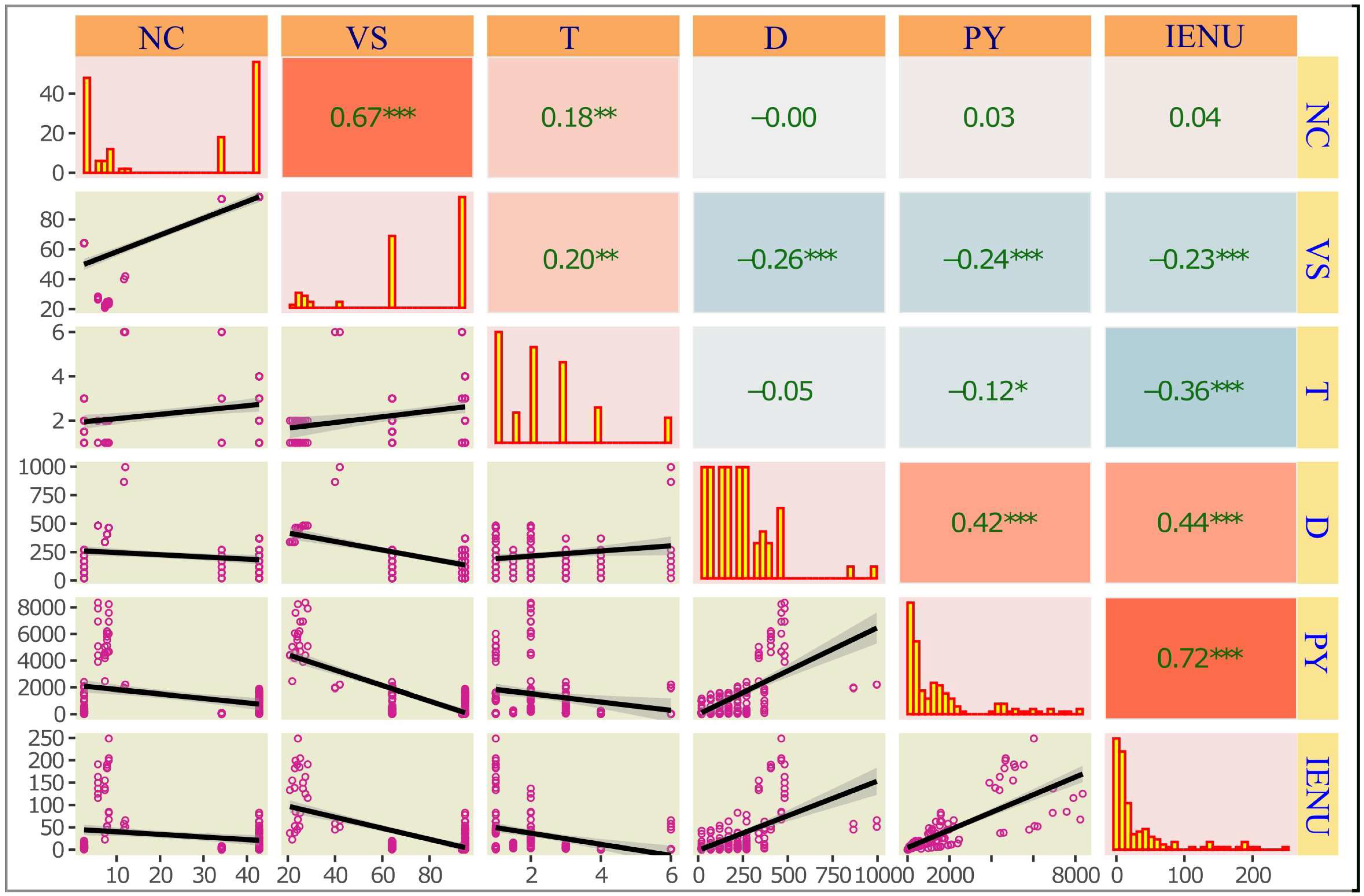
3.1. Exploratory Data Analysis

Table 2. Summary statistics of key variables in the original data.

Variable	Unit	Mean ± SD	Range (Min–Max)	CV (%)
N content (NC)	g/kg TS	24.05 ± 15.54	1.78–57.10	64.62
Volatile solids (VS)	%	55.38 ± 31.65	1.23–95.00	57.15
Growth time (T)	Month	8.17 ± 16.00	0.50–100.00	195.84
Dosage (D)	kg N/ ha	189.27 ± 181.05	0.10–1020	95.7
Plant yield (PY)	kg/ ha	2268.42 ± 3099.00	0.00–18,008.11	136.61
Internal efficiency of nitrogen utilization (IENU)	kg N/ ha	32.26 ± 92.51	0.00–1285.71	286.76

TS: Total solids; CV: Coefficient of Variation.

encompasses six variables, each capturing distinct dimensions of agricultural research. The targets, PY and IENU, exhibit high variability with coefficients of variation (CV) of 136.61% and 286.76%, respectively. PY, with a mean of 2268.42 kg TS/ha and a range up to 18,008.11 kg TS/ha, and IENU, averaging 32.26 kg N/ha with a range extending to 1285.71 kg N/ha, underscore the broad spectrum of outcomes in agricultural productivity and efficiency. Predictor variables NC, T, and D also show significant variability.

Table 3. Distribution of crop studies utilizing kitchen waste as fertilizer.

Crop	Frequency (%)
Barley (Hordeum vulgare L.)	0.45
Corn	0.45
Grass	10.76
Grass—Festuca arundinacea	0.90
Lactuva sativa	1.79
Lettuce	2.02
Oats combined	4.87
Potato (Solanum tuberosum L. ‘Dansyakuimo’)	1.35
Rice Oryza sativa L. cv. Saechucheong	0.67
Ryegrass	73.77
Shoots Kai choy (Brassica juncea, var. Hirayama)	0.67
Triple mix (a mixture of 70% timothy (Phleum pretense) + 15% red clover + 15% alsike) TM	0.22
Wheat combined	1.34
Oat combined with hairy vetch OHV	0.22
Oat combined with red clover Trifolium pretense ORC	0.22

outlines the frequency of various crops studied for growth using kitchen waste as fertilizer, reflecting multiple agricultural interests. Ryegrass dominates the dataset with a substantial frequency of 73.77%. “Grass” (unspecified species) accounted for 10.76%, while oats and lettuce followed with frequencies of 4.87% and 2.02%, respectively. Other crops, including barley, corn, and specific varieties of potato and rice, were less frequently represented (<2%), suggesting limited research attention on these species.

The correlation analysis was conducted using all available data. Due to the non-normal distribution and the presence of a significant number of ties, Kendall’s Tau-b was employed as it better accounts for tied ranks and has less influence on it. Among the predictors, D exhibited significant positive correlations with both PY and IENU, with r-values of 0.42 and 0.44, respectively (p < 0.01) (Figure 1). In contrast, VS and T showed negative correlations (r ≈ −0.24, p < 0.01), while NC was not significantly associated with the targets. The low intercorrelation among predictors suggests their independence, supporting their inclusion in predictive models.

The positive relationship between D and both PY and IENU suggests that longer decomposition allows for more complete nutrient mineralization and humification, enhancing nutrient availability and soil conditioning. As organic matter decomposes, labile nutrients are released and complex organic compounds are transformed into more stable humic substances, improving nutrient retention and soil structure [58]. From a practical perspective, these findings imply that optimizing decomposition time before application can improve fertilizer efficiency and crop productivity. Farmers could benefit from adjusting composting or pre-treatment durations of organic amendments to align with these insights, especially under resource-constrained conditions where maximizing input efficiency is critical [59,60].

3.2. Prediction of Plant Yield

The initial dataset comprises 420 rows and includes four variables: NC, T, D, and PY. Following this omission, the dataset underwent several transformations, yielding four distinct versions tailored for detailed comparative studies. These versions are denoted as Data 1 (382 cases), Data 2 (324 cases), Data 3 (324 cases), and Data 4 (299 cases). These processed datasets were each randomly divided, allocating 80% of the cases to a training set and the remaining 20% to a testing set. To ensure consistent distributions of the target variable, mitigate data leakage, identify biases, and promote model generalization, the practice of checking the distributions of training and test data in ML prediction was implemented. The histograms illustrate the PY frequency distributions across four datasets, revealing right-skewed patterns in all training sets. Notably, Data 2 is the most promising for predictive modeling due to its training and test set distributions aligning more closely (Figure S1).

3.2.1. Linear Regression

LR models applied to the four datasets produced R² values ranging from 0.18 to 0.41 (

Table 4. Multiple linear regression models for PY prediction.

Data	Phase	Model	Equation	R2	RSE	AIC	RMSE
Data 1	Training	PY~D + T + N	PY = 2.05 D + 96.84 T − 63.16 NC + 3008.99	0.24	2832	5739.00
	Testing	Trained model					2430.10
Data 2 *	Training	PY~D + T + N	PY = 2.94 D + 62.42 T − 8.05 NC + 745.50	0.41	739.7	3793.86
	Testing						759.30
Data 3	Training	PY~D + T + N	PY = 1.74 D + 76.76 T − 46.28 NC + 569.14	0.18	2877	4343.30
	Testing						2422.05
Data 4	Training	PY~D + T + N	PY = 2.89 D + 58.25 T − 11.41 NC + 1347.47	0.32	573.4	3735.80
	Testing						1263.57

* Results with normalized, log, and standardized transformation of predictors are the same.

), indicating limited explanatory power. Data 2 and 4, in particular, exhibited lower AIC values, suggesting a more suitable balance between fit and complexity than those for Data 1 and 3. However, introducing RMSE provides additional insight into the model’s predictive performance, with Data 2 and 4 showing lower errors, thus reinforcing their efficacy.

Despite the moderate explanatory power demonstrated by all models, the consistency in results between the transformed and untransformed predictors for Data 2 underscores the model’s robustness (lowest RSE, AIC, and RMSE). This aspect is particularly noteworthy as it highlights the model’s capability to effectively capture the underlying relationship between the predictors and PY, regardless of the scale or distribution of the predictor variables. However, the model’s explanatory power is limited, as the three variables collectively explain only 24% of the variation in the data. Analysis of the coefficients reveals that T has the most substantial impact on PY (62.42), followed by NC (−8.05), and then D (2.05).

The diminished predictive capacity of LR underscores the need for advanced modeling techniques to more accurately estimate PY in the context of highly variable crop yield data characterized by high variability and multifactorial influences [61,62]. LR typically yields modest results in such scenarios [63]. Moreover, the inherent variability in crop yield, characterized by its specificity to each period and its intrinsic nonlinearity, further complicates prediction [64].

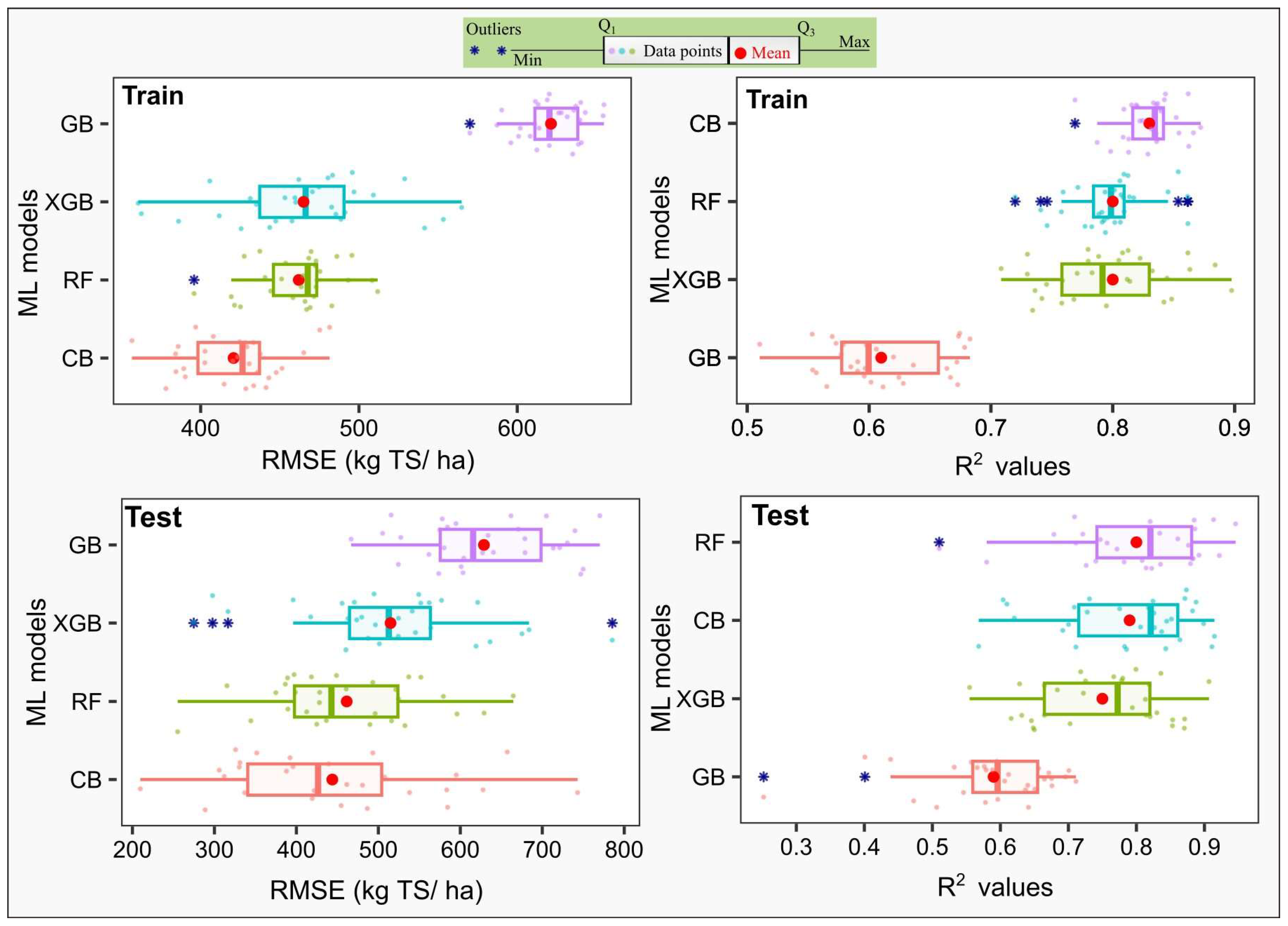
3.2.2. Machine Learning

Initially, ML algorithms, including CB, XGB, RF, and GB, were employed to identify the most suitable dataset for PY prediction. Significant differences in model performance were observed across the four datasets (

Table 5. The mean result of different ML algorithms across four datasets.

Data	Metric	XGB	RF	CB	GB
Data 1	RMSE	1229.65 a	1297.74 a	1142.77 a	1509.56 a
	R2	0.86	0.84	0.88	0.79
Data 2	RMSE	505.16 a	493.22 a	494.71 a	651.19 b
	R2	0.75	0.77	0.76	0.57
Data 3	RMSE	1460.60 a	1577.07 a	1422.36 a	1929.11 b
	R2	0.79	0.76	0.80	0.65
Data 4	RMSE	793.13 a	809.99 a	709.77 a	1111.26 b
	R2	0.78	0.76	0.82	0.58

Superscript letters (a, b) indicate statistically significant differences in RMSE within each dataset based on Tukey HSD post-hoc tests (p < 0.05). Values sharing the same letter are not significantly different.

), indicating the strong influence of data characteristics such as sample size, feature variance, and data consistency. Data 2 consistently outperformed others, with the RF model yielding the lowest RMSE (493.22) and the highest R² (0.77). A one-way ANOVA confirmed significant differences in RF performance across datasets (F(3, 56) = 56.44, p < 0.001), and Tukey HSD tests showed that RMSE in Data 2 was significantly lower than in all other datasets (p < 0.001). Similarly, model comparisons within each dataset revealed no significant differences in Data 1 (p = 0.188), while in Data 2, 3, and 4, GB consistently had significantly higher RMSE than the other models (p < 0.01), with no significant differences among XGB, RF, and Cubist. Model characteristics can explain these differences: RF and CB, which use ensemble averaging and rule-based refinement, are more robust to noise and small sample sizes. XGB, benefiting from regularization, handled clean datasets well. GB’s sequential learning made it more prone to overfitting noisy or inconsistent data. Thus, Data 2’s cleaner structure allowed models, especially RF and CB, to generalize more effectively, confirming it as the most suitable for PY prediction.

To enhance the rigor of our analysis of Data 2, four ML models were trained using 80% of the data and the remaining 20% for testing. However, due to the random nature of the split, each 80/20 split varied, leading to inconsistent model performance outcomes. To ensure robustness and reduce variance, 30 separate runs of the train/test splits were conducted, and the results were reported as the mean of these runs. This methodology aligns with the approach used by [65], who applied a similar strategy in their study using RF to predict soybean yield; however, they also included multiple repetitions to optimize hyperparameters. Each run involved training and tuning the ML models using 10-fold cross-validation and normalization transformations (Table S1). The RF and CB models demonstrated superior generalization capabilities, maintaining both high R² values (0.79–0.83) and low RMSE across training and testing sets (Figure 2). These models handle noise and nonlinear interactions well due to their ensemble structures and averaging mechanisms, making them robust against overfitting and suitable for relatively small and heterogeneous datasets.

In contrast, XGB and GB, although effective at capturing complex patterns in the training phase, showed moderate overfitting, as indicated by an increased RMSE during testing. This behavior likely stems from their boosting mechanism, which can emphasize noise if not properly regularized. Thus, their performance is more sensitive to hyperparameter tuning and data noise than RF and CB. The CB model’s effectiveness can be attributed to its rule-based structure, which excels at modeling sharp transitions and local patterns, whereas RF benefits from aggregating uncorrelated decision trees, improving stability. The optimal settings included 50 committees, one CB neighbor, and 100 trees, with mtry = 2 for RF.

Previous research has employed various techniques and predictors in ML models for estimating PY, including cross-sectional and time-series predictions and predictors based on remote sensing and ground truth data (experimental plot-based designs) [65,66]. These diverse approaches have led to inconsistent findings and varying performance levels in ML models for PY prediction. For example, RF and Support Vector Machine models showed similar efficacy, capturing between 50% and 70% of the spatial and temporal variance in yields for crops such as silage maize, winter barley, winter rapeseed, and winter wheat [67]. Furthermore, deep learning and RF models demonstrated strong performance at the field level for large-scale crop yield estimation, achieving mean R² values of 0.71 and 0.66 and RMSE values of 1127 kg/ha and 956 kg/ha, respectively [68]. The RF model in particular presented promising results in wheat yield prediction, with an RMSE of 434, normalized RMSE of 0.149 g per plot, and an R² of 0.74 [69].

3.3. Prediction of IENU

The initial dataset contains 341 entries with four variables: NC, T, D, and PY. It was transformed into four distinct versions to facilitate comparative analysis: Data 1 (302 entries), Data 2 (256 entries), Data 3 (341 entries), and Data 4 (286 entries). Histograms demonstrated the distribution quality within these datasets (Figure S2). Notably, Data 2 and Data 4 were identified as the most suitable for predictive modeling due to the close alignment between their training and testing distributions. The removal of outliers rendered the data more effective for predicting IENU.

3.3.1. Linear Regression

Data 2 exhibited the lowest testing RMSE (8.29), suggesting accurate predictions, and a comparatively low training RSE (6.864), indicating a robust model fit. Data 4, with a testing RMSE of 7.82, outperformed Data 2 in testing accuracy but has a slightly higher training RSE of 8.073, though still below Data 3’s. Conversely, Data 1 showed the poorest performance, with the highest testing RMSE (66.86) and training RSE (90.78), indicating the least accurate predictions and model fit. Data 3, despite the highest R² value during testing, also had high testing RMSE (45.96) and training RSE (98.55), reflecting lower accuracy and fit (

Table 6. Single and multiple linear regression models for IENU prediction.

Data	Phase	Model	Equation	R2	RSE	AIC	RMSE
Data 1	Training	IENU~D + T + N	IENU = −0.03D + 36.56T − 1.97NC – 0.39	0.28	95.4	2325.03	-
	Testing	Trained model					71.57
Data 2	Training	IENU~D + T + N	IENU = 9.62 + 0.03D − 2.96T + 0.12NC	0.29	6.87	1398.00	-
	Testing	Trained model					8.29
Data 3	Training	IENU~D + T + N	IENU = 45.06 + 0.05D + 0.51T − 0.87NC	0.02	92.76	3254.10	-
	Testing	Trained model					45.96
Data 4	Training	IENU~D + T + N	IENU = 7.06 − 0.01D − 0.21T + 0.10NC	0.1	7.61	1592.23	-
	Testing	Trained model					8.38

).

Overall, Data 2 was the top performer, effectively balancing prediction accuracy and model fit, while Data 4 served as a viable alternative, although its low R² value indicates sensitivity in this metric. Despite the moderate explanatory power demonstrated by all models, the model’s explanatory power is limited, as the three variables collectively explain only 27% of the variation in the data. In contrast, a multiple LR study by [70] accounted for 74% of the variation in nitrogen use efficiency. Analysis of the coefficients reveals that T had the most substantial impact on IENU (2.96), followed by NC (0.12), and then D (0.03).

3.3.2. Machine Learning

The analysis revealed that Data 2 consistently yielded the best predictive performance across all regression models, especially in the XGB and CB model, with an average RMSE of 3.91 and R² of 0.81 (

Table 7. The mean result of different ML algorithms across four datasets for IENU prediction.

Data	Metric	XGB	RF	CB	GB
Data 1	RMSE	53.38 a	63.40 a	55.06 a	61.07 a
	R2	0.67	0.47	0.70	0.54
Data 2	RMSE	3.91 a	3.97 a	3.98 a	5.58 b
	R2	0.81	0.80	0.79	0.60
Data 3	RMSE	51.33 a	63.02 a	56.38 a	60.99 a
	R2	0.74	0.52	0.68	0.59
Data 4	RMSE	4.47 a	4.48 a	4.19 a	5.68 a
	R2	0.72	0.71	0.74	0.56

Superscript letters (a, b) indicate statistically significant differences in RMSE within each dataset based on Tukey HSD post-hoc tests (p < 0.05). Values sharing the same letter are not significantly different.

). In contrast, Data 1 and 3 exhibited substantially higher RMSE values (e.g., 53.38–63.40 and 51.33–63.02, respectively), suggesting greater variability or data noise. One-way ANOVA on XGB RMSEs confirmed a significant effect of dataset on model performance (F(3, 56) = 7.64, p < 0.001). Post-hoc Tukey tests showed that Data 2 and 4 significantly outperformed Data 1 (p < 0.01). Data 3 was significantly worse than Data 2, but not significantly different from Data 1 or 4. These statistical findings support that Data 2 was the most suitable for IENU prediction, offering both low prediction error and strong explanatory power.

Performance differences reflect how each model interacts with the dataset characteristics. While robust and resistant to overfitting, RF could underperform with high-noise data (Data 1, 3). GB is sensitive to outliers and tends to overfit if not well-tuned, explaining its relatively weaker performance. XGB, with its built-in regularization and ability to handle missing values, showed better generalization on cleaner data (Data 2). With its rule-based refinement and regression tree structure, CB handled nonlinear relationships well, contributing to its strong performance on Data 2 and 4. These differences emphasize the importance of aligning model choice with data preprocessing strategies.

The ML models were assessed based on their performance metrics, including the mean RMSE and R², along with their respective standard deviations, for both the training and testing datasets (Figure 3). CB demonstrated the lowest mean RMSE on the training data at 3.62 ± 0.22, indicating its ability to make accurate predictions while maintaining consistency across iterations. Regarding R² on the training data, both XGB and CB achieved high mean values of 0.82, suggesting their effectiveness in explaining the variance in the training data. On the testing dataset, XGB maintained its strong performance with a mean RMSE of 3.62 and a mean R² of 0.81, indicating its capability to generalize well to unseen data. CB also performed well on the testing dataset, with a mean RMSE of 3.83 and a mean R² of 0.78. These results suggest that both XGB and CB exhibited promising performance in capturing the underlying patterns in the training data and making accurate predictions on new, unseen data. RF and GB models also demonstrated competitive performance, with mean RMSE values of 3.76 and 5.10, respectively, and mean R² values of 0.80 and 0.62, respectively, on the training dataset. However, their performance slightly decreased on the testing dataset, indicating potential overfitting or a lack of generalization ability compared to XGB and CB. While no studies have targeted predicting IENU precisely, several researchers have focused on nitrogen use efficiency [71,72,73]. However, the metrics used in these studies are not directly comparable to those needed in this context. The results presented here build on the study by [13], which applied only the Monod model to predict plant dry matter yield (kg d.m./ha) at each harvest based on plant nitrogen (N) utilization data (kg N/ha). The model, fitted to all available data, showed a strong overall fit, suggesting that nitrogen effectively drives yield dynamics. However, since Monod was applied to the entire dataset without independent validation, there is a risk of overfitting. As a result, its predictive accuracy for new, unseen inputs remains uncertain and may lead to incorrect estimations under different conditions.

4. Limitations and Practical Applications

4.1. Limitations

This research, while innovative, has several limitations that future studies need to address. First, the data variability and completeness issues stem primarily from the datasets gathered through controlled experiments, which may not capture the full variability and complexities of real-world agricultural settings. Future research should incorporate more diverse, field-based datasets across varying climatic zones, soil types, and farming practices to improve generalizability. This would help validate the models under real-world conditions and enhance their robustness. Additionally, the high rate of missing data and the exclusion of certain variables could impact the robustness and generalizability of the findings. Second, the ML models, despite showing promising results, carry a potential risk of overfitting, particularly noted in models like XGB and Gradient Boosting when applied to unseen data. Enhancing the models’ generalization capabilities to various agricultural environments remains critical for future research. Third, the experiments were conducted on a relatively small scale, and scaling these findings to more extensive commercial agricultural operations could introduce new challenges, such as logistical, economic, and climatic variations that were not accounted for in this study. Lastly, the effectiveness of FW-derived fertilizers is heavily dependent on the specific pre-treatment processes used, and different treatments may yield varying effectiveness across different soil types and crop species, which this study did not fully explore.

4.2. Practical Applications

Despite the limitations above, this study offers valuable insights with significant practical applications. It supports the shift towards more sustainable agricultural practices by demonstrating the effectiveness of FW-derived fertilizers, encouraging recycled organic waste, reducing reliance on chemical fertilizers, and minimizing environmental impact. The findings can help inform policymakers in developing guidelines and regulations that promote organic waste recycling into valuable agricultural inputs, encouraging circular economy practices in the farming sector [74].

The predicted outcomes for PY and IENU offer practical decision-support tools for farmers and gardeners. By inputting site-specific parameters (e.g., fertilizer dose, plant type, growth period), users can obtain data-driven recommendations to optimize fertilizer strategies—maximizing yield and nitrogen use efficiency while minimizing waste. These predictions support precision agriculture by guiding application rates and timing, tailored to crop and soil conditions. Furthermore, accurate yield estimates enhance resource planning (e.g., labor and equipment) and help manage risks related to yield variability and market fluctuations, ultimately improving operational efficiency and sustainability. The application of ML models in predicting the outcomes of different fertilizer treatments can aid farmers and agricultural practitioners in optimizing the use of resources. This optimization leads to better crop yields and more efficient use of nitrogen, enhancing food security and sustainability.

To improve accessibility, these models can be integrated into mobile or web-based applications that assist farmers in real time, providing tailored fertilizer plans based on local conditions. ML has recently been gradually used to develop decision support tools for modern agricultural systems, covering nutrient management to improve yields while reducing expenses and environmental impact [66]. It can provide cost-effective and thorough nutrient assessment and decision-making solutions [75,76].

Additionally, integrating ML into agricultural practices offers an excellent opportunity for educational programs to teach new technologies in agronomy, fostering a new generation of tech-savvy farmers and researchers. Lastly, there is potential for commercializing the FW treatment processes and the related ML prediction models developed in this study. These can be offered to agricultural businesses as part of a service or technology package, enhancing their productivity and environmental sustainability.

5. Conclusions

This study provides key insights into the potential of FW-derived fertilizers for agronomic effectiveness and predicting PY and IENU via data-driven models. By rigorously filtering out missing values and outliers, Data 2 delivered reliable and consistent results. Correlation analysis revealed that decomposition duration positively impacted PY and IENU, while temperature and volatile solids had negative correlations. ML models outperformed linear regression, with RF yielding accurate predictions for PY and CB and XGB performing best for IENU. By integrating predictive simulations into fertilization planning, this study contributes to sustainable agriculture by enhancing resource efficiency and reducing reliance on synthetic fertilizers. Future research should explore larger datasets and additional environmental factors to refine ML-based fertilizer optimization strategies.

References

1. Álvarez Salas, M.; Sica, P.; Rydgård, M.; Sitzmann, T.J.; Nyang’au, J.O.; El Mahdi, J.; Moshkin, E.; de Castro e Silva, H.L.; Chrysanthopoulos, S.; Kopp, C.; et al. Current challenges on the widespread adoption of new bio-based fertilizers: Insights to move forward toward more circular food systems. Front. Sustain. Food Syst. 2024, 8, 1386680. [Google Scholar] [CrossRef]
2. Steffens, M.; Bünemann, E.K. Quality of bio-based fertilizers is decisive for improving soil quality in Europe—A meta-analysis. Soil Use Manag. 2025, 41, e70012. [Google Scholar] [CrossRef]
3. O’Connor, J.; Hoang, S.A.; Bradney, L.; Rinklebe, J.; Kirkham, M.B.; Bolan, N.S. Value of dehydrated food waste fertiliser products in increasing soil health and crop productivity. Environ. Res. 2022, 204, 111927. [Google Scholar] [CrossRef] [PubMed]
4. Cheong, J.C.; Lee, J.T.E.; Lim, J.W.; Song, S.; Tan, J.K.N.; Chiam, Z.Y.; Yap, K.Y.; Lim, E.Y.; Zhang, J.; Tan, H.T.W.; et al. Closing the food waste loop: Food waste anaerobic digestate as fertilizer for the cultivation of the leafy vegetable, xiao bai cai (Brassica rapa). Sci. Total Environ. 2020, 715, 136789. [Google Scholar] [CrossRef]
5. Gao, S.; Lu, D.; Qian, T.; Zhou, Y. Thermal hydrolyzed food waste liquor as liquid organic fertilizer. Sci. Total Environ. 2021, 775, 145786. [Google Scholar] [CrossRef]
6. The World Counts. Global Challenges. 2022. Available online: https://www.theworldcounts.com/challenges/people-and-poverty/hunger-and-obesity/food-waste-statistics (accessed on 15 December 2024).
7. FAO. “Energy-Smart” Food for People and Climate: Issue Paper; Food and Agriculture Organization of the United Nations: Rome, Italy, 2011. [Google Scholar]
8. Elgarahy, A.M.; Eloffy, M.G.; Alengebawy, A.; El-Sherif, D.M.; Gaballah, M.S.; Elwakeel, K.Z.; El-Qelish, M. Sustainable management of food waste; pre-treatment strategies, techno-economic assessment, bibliometric analysis, and potential utilizations: A systematic review. Environ. Res. 2023, 225, 115558. [Google Scholar] [CrossRef]
9. Razouk, A.; Tiganescu, E.; von Glahn, A.J.; Abdin, A.Y.; Nasim, M.J.; Jacob, C. The future in the litter bin—Bioconversion of food waste as driver of a circular bioeconomy. Front. Nutr. 2024, 11, 1325190. [Google Scholar] [CrossRef]
10. Meng, X.; Zeng, B.; Wang, P.; Li, J.; Cui, R.; Ren, L. Food waste anaerobic biogas slurry as fertilizer: Potential salinization on different soil layer and effect on rhizobacteria community. Waste Manag. 2022, 144, 490–501. [Google Scholar] [CrossRef]
11. Song, S.; Lim, J.W.; Lee, J.T.E.; Cheong, J.C.; Hoy, S.H.; Hu, Q.; Tan, J.K.N.; Chiam, Z.; Arora, S.; Lum, T.Q.H.; et al. Food-waste anaerobic digestate as a fertilizer: The agronomic properties of untreated digestate and biochar-filtered digestate residue. Waste Manag. 2021, 136, 143–152. [Google Scholar] [CrossRef]
12. Siddiqui, Z.; Hagare, D.; Jayasena, V.; Swick, R.; Rahman, M.M.; Boyle, N.; Ghodrat, M. Recycling of food waste to produce chicken feed and liquid fertiliser. Waste Manag. 2021, 131, 386–393. [Google Scholar] [CrossRef]
13. Kuligowski, K.; Konkol, I.; Świerczek, L.; Chojnacka, K.; Cenian, A.; Szufa, S. Evaluation of Kitchen Waste Recycling as Organic N-Fertiliser for Sustainable Agriculture under Cool and Warm Seasons. Sustainability 2023, 15, 7997. [Google Scholar] [CrossRef]
14. Yang, X.; Nguyen, X.C.; Tran, Q.B.; Huyen Nguyen, T.T.; Ge, S.; Nguyen, D.D.; Nguyen, V.T.; Le, P.C.; Rene, E.R.; Singh, P.; et al. Machine learning-assisted evaluation of potential biochars for pharmaceutical removal from water. Environ. Res. 2022, 214, 113953. [Google Scholar] [CrossRef] [PubMed]
15. Nguyen, X.C.; Bui, V.K.H.; Cho, K.H.; Hur, J. Practical application of machine learning for organic matter and harmful algal blooms in freshwater systems: A review. Crit. Rev. Environ. Sci. Technol. 2023, 54, 953–975. [Google Scholar] [CrossRef]
16. Balasubramanian, P.; Prabhakar, M.R.; Liu, C.; Li, F.; Nguyen, X.C.; Nageshwari, K.; Zhang, Z.; Zhang, P. Predictive Capability of Phosphate Recovery from Wastewater Using a Rough Set Machine Learning Model. ACS EST Eng. 2024, 4, 2449–2459. [Google Scholar] [CrossRef]
17. Nguyen, X.C.; Ly, Q.V.; Peng, W.; Nguyen, V.H.; Nguyen, D.D.; Tran, Q.B.; Huyen Nguyen, T.T.; Sonne, C.; Lam, S.S.; Ngo, H.H.; et al. Vertical flow constructed wetlands using expanded clay and biochar for wastewater remediation: A comparative study and prediction of effluents using machine learning. J. Hazard. Mater. 2021, 413, 125426. [Google Scholar] [CrossRef]
18. Li, X.; Dai, W.; Gao, H.; Xu, W.; Wei, X. Correlation between Grain Yield and Fertilizer Use Based on Back Propagation Neural Network. Nongye Jixie Xuebao/Trans. Chin. Soc. Agric. Mach. 2017, 48, 186–192. [Google Scholar] [CrossRef]
19. Wang, F.; Dong, Z.; Wu, Z.; Fang, K. Optimization of maize planting density and fertilizer application rate based on BP neural network. Trans. Chin. Soc. Agric. Eng. 2017, 33, 92–99. [Google Scholar] [CrossRef]
20. Meng, L.; Liu, H.; Ustin, S.L.; Zhang, X. Predicting maize yield at the plot scale of different fertilizer systems by multi-source data and machine learning methods. Remote Sens. 2021, 13, 3760. [Google Scholar] [CrossRef]
21. Thai, T.H.; Omari, R.A.; Barkusky, D.; Bellingrath-Kimura, S.D. Statistical analysis versus the m5p machine learning algorithm to analyze the yield of winter wheat in a long-term fertilizer experiment. Agronomy 2020, 10, 1779. [Google Scholar] [CrossRef]
22. Santa-María, G.E.; Moriconi, J.I.; Oliferuk, S. Internal efficiency of nutrient utilization: What is it and how to measure it during vegetative plant growth? J. Exp. Bot. 2015, 66, 3011–3018. [Google Scholar] [CrossRef]
23. Rochester, I.J. Assessing internal crop nitrogen use efficiency in high-yielding irrigated cotton. Nutr. Cycl. Agroecosystems 2011, 90, 147–156. [Google Scholar] [CrossRef]
24. Kuligowski, K.; Konkol, I.; Świerczek, L.; Woźniak, A.; Cenian, A. Conversion of Kitchen Waste into Sustainable Fertilizers: Comparative Effectiveness of Biological, Microbial, and Thermal Treatments in a Ryegrass Growth Trial. Appl. Sci. 2025, 15, 5281. [Google Scholar] [CrossRef]
25. Lee, J.-J.; Park, R.-D.; Kim, Y.-W.; Shim, J.-H.; Chae, D.-H.; Rim, Y.-S.; Sohn, B.-K.; Kim, T.-H.; Kim, K.-Y. Effect of food waste compost on microbial population, soil enzyme activity and lettuce growth. Bioresour. Technol. 2004, 93, 21–28. [Google Scholar] [CrossRef]
26. Tampio, E.; Salo, T.; Rintala, J. Agronomic characteristics of five different urban waste digestates. J. Environ. Manag. 2016, 169, 293–302. [Google Scholar] [CrossRef] [PubMed]
27. Gondek, K.; Filipek-Mazur, B. Accumulation of microelements in oat biomass and their availability in soil fertilised with compost of plant wastes. Acta Agrophysica 2006, 8, 579–590. (In Polish) [Google Scholar]
28. Keeling, A.A.; Griffiths, B.S.; Ritz, K.; Myers, M. Effects of compost stability on plant growth, microbiological parameters and nitrogen availability in media containing mixed garden-waste compost. Bioresour. Technol. 1995, 54, 279–284. [Google Scholar] [CrossRef]
29. Cordovil, C.M.; Cabral, F.; Coutinho, J. Potential mineralization of nitrogen from organic wastes to ryegrass and wheat crops. Bioresour. Technol. 2007, 98, 3265–3268. [Google Scholar] [CrossRef]
30. Gondek, K.; Filipek-Mazur, B. Fertilization Value of Green Waste Compost from Krakow. Probl. Books Prog. Agric. Sci. 2003, 494, 113–121. [Google Scholar]
31. Jasiewicz, C.; Antonkiewicz, J.; Baran, A. The Effect of Fertilization on Yielding and Nitrogen Content in Tall Oat Grass. Probl. Books Prog. Agric. Sci. 2006, 513, 149. (In Polish) [Google Scholar]
32. Wiater, J. The Sequent Impact of Organic Wastes on Yielding and Chemical Composition of Winter Whea. Probl. Books Prog. Agric. Sci. 2003, 494, 525–532. [Google Scholar]
33. Martyniak, D.; Prokopiuk, K.; Żurek, G.; Rybka, K. Measuring Fluorescence as a Means to Evaluate the Physiological Reaction to Growth Retardant Applied to Manage Turf. Agronomy 2022, 12, 1776. [Google Scholar] [CrossRef]
34. Jasiewicz, C.; Antonkiewicz, J. The Effect of a Dose and Kind of Fertilizer on Maize Nitrogen Concentration. In Proceedings of the Environmental Pollution by Nitrogen, Olecko, Poland; 2005. Date not available publication in Polish. [Google Scholar]
35. Jamison, J.; Khanal, S.K.; Nguyen, N.H.; Deenik, J.L. Assessing the Effects of Digestates and Combinations of Digestates and Fertilizer on Yield and Nutrient Use of Brassica juncea (Kai Choy). Agronomy 2021, 11, 509. [Google Scholar] [CrossRef]
36. Sullivan, D.M.; Bary, A.I.; Thomas, D.R.; Fransen, S.C.; Cogger, C.G. Food Waste Compost Effects on Fertilizer Nitrogen Efficiency, Available Nitrogen, and Tall Fescue Yield. Soil Sci. Soc. Am. J. 2002, 66, 154–161. [Google Scholar] [CrossRef]
37. Simon, F.; Junior, A.; Loss, A.; Malinowski, C.; Matias, M. Effects of food waste digested materials on Lactuva sativa growth and soil composition. Int. J. Environ. Sci. Technol. 2022, 20, 9013–9028. [Google Scholar] [CrossRef]
38. Messiga, A.J.; Sharifi, M.; Munroe, S. Combinations of cover crop mixtures and bio-waste composts enhance biomass production and nutrients accumulation: A greenhouse study. Renew. Agric. Food Syst. 2016, 31, 507–515. [Google Scholar] [CrossRef]
39. Sung, J.; Kim, W.; Oh, T.-K.; So, Y.-S. Nitrogen (N) use efficiency and yield in rice under varying types and rates of N source: Chemical fertilizer, livestock manure compost and food waste-livestock manure compost. Appl. Biol. Chem. 2023, 66, 4. [Google Scholar] [CrossRef]
40. Dragicevic, I.; Sogn, T.A.; Eich-Greatorex, S. Recycling of Biogas Digestates in Crop Production—Soil and Plant Trace Metal Content and Variability. Front. Sustain. Food Syst. 2018, 2, 45. [Google Scholar] [CrossRef]
41. Asagi, N.; Minamide, K.; Uno, T.; Saito, M.; Ito, T. Acidulocompost, a food waste compost with thermophilic lactic acid fermentation: Its effects on potato production and weed growth. Plant Prod. Sci. 2016, 19, 132–144. [Google Scholar] [CrossRef]
42. Gondek, K.; Filipek-Mazur, B. Agro-chemical assessment of fertilizer value of composts of various origin. Acta Agrophysica 2005, 5, 271–282. (In Polish) [Google Scholar]
43. Friedman, J.H. Greedy function approximation: A gradient boosting machine. Ann. Stat. 2001, 29, 1189–1232. [Google Scholar] [CrossRef]
44. Du, Z.; Yang, L.; Zhang, D.; Cui, T.; He, X.; Xiao, T.; Xie, C.; Li, H. Corn variable-rate seeding decision based on gradient boosting decision tree model. Comput. Electron. Agric. 2022, 198, 107025. [Google Scholar] [CrossRef]
45. Quinlan, J.R. Combining instance-based and model-based learning. In Proceedings of the Tenth International Conference on International Conference on Machine Learning, Amherst, MA, USA, 13–19 July 1993; pp. 236–243. [Google Scholar]
46. Quinlan, J.R. Learning with continuous classes. In Proceedings of the 5th Australian Joint Conference on Artificial Intelligence, Hobart, Tasmania, 16–18 November 1992; pp. 343–348. [Google Scholar]
47. Kuhn, M.; Johnson, K. Applied Predictive Modeling; Springer: New York, NY, USA, 2013; pp. 101–139. [Google Scholar]
48. Nguyen, X.C.; Nguyen, T.T.H.; La, D.D.; Kumar, G.; Rene, E.R.; Nguyen, D.D.; Chang, S.W.; Chung, W.J.; Nguyen, X.H.; Nguyen, V.K. Development of machine learning—Based models to forecast solid waste generation in residential areas: A case study from Vietnam. Resour. Conserv. Recycl. 2021, 167, 105381. [Google Scholar] [CrossRef]
49. Chen, T.; Guestrin, C. XGBoost: A Scalable Tree Boosting System. In Proceedings of the 22nd ACM SIGKDD International Conference on Knowledge Discovery and Data Mining, San Francisco, CA, USA, 13–17 August 2016; pp. 785–794. [Google Scholar]
50. Naghdyzadegan Jahromi, M.; Zand-Parsa, S.; Razzaghi, F.; Jamshidi, S.; Didari, S.; Doosthosseini, A.; Pourghasemi, H. Developing machine learning models for wheat yield prediction using ground-based data, satellite-based actual evapotranspiration and vegetation indices. Eur. J. Agron. 2023, 146, 126820. [Google Scholar] [CrossRef]
51. Huber, F.; Yushchenko, A.; Stratmann, B.; Steinhage, V. Extreme Gradient Boosting for yield estimation compared with Deep Learning approaches. Comput. Electron. Agric. 2022, 202, 107346. [Google Scholar] [CrossRef]
52. Islam, A.; Khair, I.; Ifty, R.A.; Hossain, S.; Arefin, M.N.; Abid, F.B.A. Bangladeshi Agricultural Product Forecasting Approach Using Permutation Driven Machine Learning Algorithm. In Proceedings of the 2022 International Conference on Recent Progresses in Science, Engineering and Technology (ICRPSET), Rajshahi, Bangladesh, 26–27 December 2022; pp. 1–6. [Google Scholar]
53. Breiman, L. Random Forests. Mach. Learn. 2001, 45, 5–32. [Google Scholar] [CrossRef]
54. Belgiu, M.; Drăguţ, L. Random forest in remote sensing: A review of applications and future directions. ISPRS J. Photogramm. Remote Sens. 2016, 114, 24–31. [Google Scholar] [CrossRef]
55. Akaike, H. A New Look at the Statistical Model Identification. In Selected Papers of Hirotugu Akaike; Parzen, E., Tanabe, K., Kitagawa, G., Eds.; Springer: New York, NY, USA, 1998; pp. 215–222. [Google Scholar]
56. Montgomery, D.C.; Peck, E.A.; Vining, G.G. Introduction to Linear Regression Analysis; John Wiley & Sons: Hoboken, NJ, USA, 2021. [Google Scholar]
57. Nguyen, X.C.; Nguyen, T.P.; Lam, V.S.; Le, P.C.; Vo, T.D.H.; Hoang, T.H.T.; Chung, W.J.; Chang, S.W.; Nguyen, D.D. Estimating ammonium changes in pilot and full-scale constructed wetlands using kinetic model, linear regression, and machine learning. Sci. Total Environ. 2024, 907, 168142. [Google Scholar] [CrossRef]
58. Bernal, M.P.; Alburquerque, J.A.; Moral, R. Composting of animal manures and chemical criteria for compost maturity assessment. A review. Bioresour. Technol. 2009, 100, 5444–5453. [Google Scholar] [CrossRef] [PubMed]
59. Gianico, A.; Gallipoli, A.; Montecchio, D.; Mininni, G. Land Application of Biosolids in Europe: Possibilities, Con-Straints and Future Perspectives. Water 2021, 13, 103. [Google Scholar] [CrossRef]
60. Li, R.; Wang, J.J.; Zhang, Z.; Shen, F.; Zhang, G.; Qin, R.; Li, X.; Xiao, R. Nutrient transformations during composting of pig manure with bentonite. Bioresour. Technol. 2012, 121, 362–368. [Google Scholar] [CrossRef]
61. Pantazi, X.E.; Moshou, D.; Alexandridis, T.; Whetton, R.L.; Mouazen, A.M. Wheat yield prediction using machine learning and advanced sensing techniques. Comput. Electron. Agric. 2016, 121, 57–65. [Google Scholar] [CrossRef]
62. Rashid, M.; Bari, B.S.; Yusup, Y.; Kamaruddin, M.A.; Khan, N. A Comprehensive Review of Crop Yield Prediction Using Machine Learning Approaches with Special Emphasis on Palm Oil Yield Prediction. IEEE Access 2021, 9, 63406–63439. [Google Scholar] [CrossRef]
63. Emamgholizadeh, S.; Parsaeian, M.; Baradaran, M. Seed yield prediction of sesame using artificial neural network. Eur. J. Agron. 2015, 68, 89–96. [Google Scholar] [CrossRef]
64. Whetton, R.; Zhao, Y.; Shaddad, S.; Mouazen, A.M. Nonlinear parametric modelling to study how soil properties affect crop yields and NDVI. Comput. Electron. Agric. 2017, 138, 127–136. [Google Scholar] [CrossRef]
65. Santos, L.B.; Gentry, D.; Tryforos, A.; Fultz, L.; Beasley, J.; Gentimis, T. Soybean yield prediction using machine learning algorithms under a cover crop management system. Smart Agric. Technol. 2024, 8, 100442. [Google Scholar] [CrossRef]
66. van Klompenburg, T.; Kassahun, A.; Catal, C. Crop yield prediction using machine learning: A systematic literature review. Comput. Electron. Agric. 2020, 177, 105709. [Google Scholar] [CrossRef]
67. Lischeid, G.; Webber, H.; Sommer, M.; Nendel, C.; Ewert, F. Machine learning in crop yield modelling: A powerful tool, but no surrogate for science. Agric. For. Meteorol. 2022, 312, 108698. [Google Scholar] [CrossRef]
68. Cao, J.; Zhang, Z.; Luo, Y.; Zhang, L.; Zhang, J.; Li, Z.; Tao, F. Wheat yield predictions at a county and field scale with deep learning, machine learning, and google earth engine. Eur. J. Agron. 2021, 123, 126204. [Google Scholar] [CrossRef]
69. Sharma, V.; Honkavaara, E.; Hayden, M.; Kant, S. UAV Remote Sensing Phenotyping of Wheat Collection for Response to Water Stress and Yield Prediction Using Machine Learning. Plant Stress 2024, 12, 100464. [Google Scholar] [CrossRef]
70. Liu, Y.; Heuvelink, G.B.M.; Bai, Z.; He, P.; Xu, X.; Ma, J.; Masiliūnas, D. Space-time statistical analysis and modelling of nitrogen use efficiency indicators at provincial scale in China. Eur. J. Agron. 2020, 115, 126032. [Google Scholar] [CrossRef]
71. Liu, J.; Zhu, Y.; Tao, X.; Chen, X.; Li, X. Rapid prediction of winter wheat yield and nitrogen use efficiency using consumer-grade unmanned aerial vehicles multispectral imagery. Front. Plant Sci. 2022, 13, 1032170. [Google Scholar] [CrossRef] [PubMed]
72. Li, Y.; Cui, S.; Zhang, Z.; Zhuang, K.; Wang, Z.; Zhang, Q. Determining effects of water and nitrogen input on maize (Zea mays) yield, water- and nitrogen-use efficiency: A global synthesis. Sci. Rep. 2020, 10, 9699. [Google Scholar] [CrossRef] [PubMed]
73. Correndo, A.A.; Rotundo, J.L.; Tremblay, N.; Archontoulis, S.; Coulter, J.A.; Ruiz-Diaz, D.; Franzen, D.; Franzluebbers, A.J.; Nafziger, E.; Schwalbert, R.; et al. Assessing the uncertainty of maize yield without nitrogen fertilization. Field Crops Res. 2021, 260, 107985. [Google Scholar] [CrossRef]
74. Chen, L.; He, P.; Zhang, H.; Peng, W.; Qiu, J.; Lü, F. Applications of machine learning tools for biological treatment of organic wastes: Perspectives and challenges. Circ. Econ. 2024, 3, 100088. [Google Scholar] [CrossRef]
75. Durai, S.K.S.; Shamili, M.D. Smart farming using Machine Learning and Deep Learning techniques. Decis. Anal. J. 2022, 3, 100041. [Google Scholar] [CrossRef]
76. Gupta, R.; Ouderji, Z.H.; Uzma, Y.Z.; Sloan, W.T.; You, S. Machine learning for sustainable organic waste treatment: A critical review. npj Mater. Sustain. 2024, 2, 5. [Google Scholar] [CrossRef]
Figure 1. Multiple plots (scatter, histogram, and Spearman correlation) for all variables in the dataset. The upper triangle displays Spearman correlation coefficients with significance levels denoted by asterisks (*, **, and ***, representing p-values ≤ 0.05, ≤0.01, and ≤0.001, respectively). The value at the intersection of the lines indicates the correlation between the variables. The lower triangle presents scatterplots for each pair of variables. The diagonal shows histograms of each variable’s distribution.
Applsci 15 05999 g001
Figure 2. Comparison results of train/test data using ML models for PY prediction (data 2).
Applsci 15 05999 g002
Figure 3. Comparison results of train/test data using ML models for IENU prediction (data 2).
Applsci 15 05999 g003