Panchromatic and Hyperspectral Image Fusion Using Ratio Residual Attention Networks

Abstract

Hyperspectral remote sensing images provide rich spectral information about land surface features and are widely used in fields such as environmental monitoring, disaster assessment, and land classification. However, effectively leveraging the spectral information in hyperspectral images remains a significant challenge. In this paper, we propose a hyperspectral pansharpening method based on ratio transformation and residual networks, which significantly enhances both spatial details and spectral fidelity. The method generates an initial image through ratio transformation and refines it using a residual attention network. Additionally, specialized loss functions are designed to preserve both spatial and spectral details. Experimental results demonstrate that, when evaluated on the EO-1 and Chikusei datasets, the proposed method outperforms other methods in terms of both visual quality and quantitative metrics, particularly in spatial detail clarity and spectral fidelity. This approach effectively addresses the limitations of existing technologies and shows great potential for high-resolution remote sensing image processing applications.

1. Introduction

Hyperspectral images contain rich spectral information about land features, which can be utilized for various applications, including remote sensing image interpretation, target detection, land classification, disaster analysis, and more [1]. In addition to traditional land-based applications, hyperspectral remote sensing has recently been extended to emerging scenarios such as solar photovoltaic plant detection and oceanic observation involving spectral variability and adjacency effects [2,3]. However, due to the limitations of physical sensors and the bandwidth constraints of information transmission, the spatial resolution of hyperspectral images is typically low. As a result, remote sensing satellites often carry multiple types of sensors to provide complementary information. In practical applications, high-resolution panchromatic images are frequently fused with low-resolution hyperspectral images to generate high-resolution hyperspectral fusion images.

Over the past few decades, image fusion technology has been extensively studied. Early image fusion methods relied on specific mathematical transformations to design fusion rules in either the spatial domain or the transformation domain, which are often referred to as traditional fusion methods. Examples of these methods include component substitution fusion [4], multi-resolution analysis fusion [5], and variational fusion [6]. Among these traditional model-based methods, Coupled Non-negative Matrix Factorization (CNMF) [7] and Hyperspectral Super-resolution (HySure) [8] stand out as representative approaches. CNMF jointly decomposes panchromatic and hyperspectral image matrices to effectively integrate spatial and spectral information, enhancing fusion quality; HySure utilizes a convex optimization framework that incorporates prior knowledge and data fidelity terms to improve spectral preservation. These methods have advanced beyond basic transform-based fusion by better preserving details and reducing artifacts, laying the groundwork for subsequent deep learning approaches. However, as research has advanced, the limitations of these methods have become increasingly evident. On the one hand, to ensure the feasibility of subsequent feature fusion, traditional methods require the same transformation to extract features from different source images. However, this approach does not account for the feature differences across source images, which may lead to poor feature representation. On the other hand, traditional feature fusion strategies are often too coarse, resulting in limited fusion performance.

In the last decade, the rise of deep learning has brought about significant changes in the field of image processing. Deep learning technologies have also been successfully applied to panchromatic and hyperspectral image fusion, addressing many challenges that traditional methods could not overcome. Zheng Y et al. [9] proposed a fusion method that combines guided filtering and residual networks for panchromatic and hyperspectral image fusion. He L et al. [10] introduced a spectral detail-preserving convolutional neural network for fusion. Dong W et al. [11] proposed a dense network based on Laplacian pyramids (DenseNet) for the fusion of panchromatic and hyperspectral images. In addition to the deep learning methods combined with traditional techniques mentioned above, many novel deep learning approaches have emerged in the field of panchromatic and hyperspectral image fusion. For example, Xie W et al. [12] designed a 3D generative adversarial network for hyperspectral image fusion. Zheng Y et al. [13] proposed a hyperspectral-panchromatic sharpening method based on deep priors and a dual-attention residual network.

In addition to earlier deep learning-based approaches, several recent methods have significantly advanced hyperspectral pansharpening since 2020. Rui et al. [14] proposed an unsupervised fusion method based on a low-rank diffusion model, which improves structural fidelity without requiring paired supervision. Shang et al. [15] introduced MFT-GAN, a multi-scale feature-guided transformer network that integrates GANs and transformer architectures to enhance spectral–spatial representation. Bandara and Patel [16] developed HyperTransformer, a fusion framework that combines both textural and spectral cues using a transformer-based design to achieve high-fidelity results. Furthermore, Deng et al. [17] proposed PSRT, a pyramid shuffle-and-reshuffle transformer that effectively captures both local and global dependencies via a hierarchical attention mechanism. Compared to these recent approaches, our method maintains a simpler residual attention architecture while achieving competitive or superior performance in both spatial detail preservation and spectral fidelity.

These deep learning-based panchromatic and hyperspectral image fusion methods typically use original hyperspectral (HS) images as labels, along with degraded panchromatic (PANLR) images and hyperspectral images (HSLR) as training samples due to the lack of high-resolution hyperspectral images for supervision during training. While these methods can achieve certain results, they overlook the specific objective of panchromatic sharpening, treating it merely as an image regression problem. They treat the panchromatic sharpening process as a black-box deep learning problem, failing to account for various real-world factors, which leads to insufficient retention of spectral and spatial information. Furthermore, using blurred or downsampled images as training samples may result in the loss of fused image information, particularly with respect to preserving spectral and spatial details. Since hyperspectral images encompass a wide spectral range and a large number of narrow-band details, existing methods are prone to spectral distortion and spatial blurring, ultimately degrading the quality of the fused image. These real-world challenges are primarily caused by the following three technical problems:

(1)

Supervised deep learning fusion methods require high-resolution hyperspectral images as labels, but such high-resolution hyperspectral images are not available in practice.

(2)

The fusion problem of panchromatic and hyperspectral images is treated as a black-box deep learning problem, where deep networks learn the mapping relationship between high-resolution and low-resolution images.

(3)

Spectral differences exist between the two images, and many continuous narrow-band details need to be analyzed, making it easy to introduce spectral distortion and spatial blurring.

To address the above issues, this paper proposes a fusion method for panchromatic and hyperspectral images that combines ratio transformations and residual networks. First, a ratio transformation method is applied to generate an initial ratio image. Next, the ratio image is input into a residual attention network, which fine-tunes the ratio image and produces a new ratio image. Finally, the generated ratio image is multiplied by the hyperspectral upsampled image to obtain the final fused image. During this process, two loss functions are designed: the spectral preservation loss function and the spatial preservation loss function, which separately constrain the spectral and spatial details of the fused image. This method does not require blurring or downsampling of the original hyperspectral images to prepare training data, effectively preserving both the spectral and spatial details of the original hyperspectral and panchromatic images.

The structure of this paper is organized as follows: Section 2 introduces the proposed fusion method and its implementation. Section 3 presents the experimental results and discusses the performance of the proposed method. Section 4 provides a discussion of the advantages and limitations of the method. Finally, Section 5 concludes the paper and summarizes its main contributions.

2. Related Work

Recent advancements in deep learning have led to significant progress in hyperspectral pansharpening. For instance, Wang et al. [18] proposed a spatial-spectral residual network that effectively captures spatial and spectral features using 3D convolutions. Wu et al. [19] introduced a distributed fusion framework based on residual CNNs, achieving improved fusion quality by leveraging multi-scale features. Guan and Lam [20] developed a multistage dual-attention guided fusion network, which employs spectral and spatial attention mechanisms to enhance fusion performance. Additionally, Xie et al. [21] presented the MS/HS Fusion Net, a model-based deep learning approach that integrates observation models with deep networks for effective fusion.

In addition to these methods, several other deep learning approaches have also demonstrated promising results. For example, He et al. [22] introduced a densely connected network that enhances feature reuse and alleviates gradient vanishing, improving the detail preservation in fused images. Zhang et al. [23] proposed an attention-based fusion network that adaptively weights spectral and spatial features, further boosting fusion accuracy. Moreover, GAN-based methods such as the one by Li et al. [24] utilize adversarial training to generate more realistic and spectrally consistent fused images.

On the other hand, traditional model-based fusion methods such as Coupled Non-negative Matrix Factorization (CNMF) [7] and Hyperspectral Super-resolution (HySure) [8] remain important baselines. CNMF jointly decomposes the hyperspectral and panchromatic data matrices to effectively integrate spatial and spectral information, while HySure employs a convex optimization framework incorporating prior knowledge and data fidelity terms to enhance spectral fidelity. Additionally, multi-resolution analysis techniques [25] have been employed to better capture features at different scales, which lays a solid foundation for subsequent deep learning fusion frameworks.

Despite these significant advances, challenges persist in simultaneously preserving fine spatial details and accurate spectral information. Many existing methods either sacrifice spectral fidelity for spatial sharpness or vice versa. To address these limitations, our proposed method introduces a novel ratio transformation combined with a residual attention network. This approach aims to effectively capture the complementary characteristics of spatial and spectral domains, leading to enhanced fused image quality with improved spatial detail and spectral fidelity.

Despite these advancements, challenges remain in effectively preserving both spatial details and spectral fidelity. Our proposed method addresses these challenges by introducing a novel ratio transformation combined with a residual attention network, aiming to enhance both the spatial and spectral aspects of fused images.

3. Methods

3.1. Framework Overview

In panchromatic and hyperspectral image fusion, effectively combining the high spatial resolution of panchromatic images with the rich spectral information of hyperspectral images remains a key challenge. To address this, this study proposes a fusion method that combines ratio transformations with residual networks. The method consists of three key components: first, a ratio transformation method is used to generate an initial ratio image, which captures the difference information between the panchromatic and hyperspectral images through ratio computation. Second, a residual attention network is employed to fine-tune the initial ratio image, using an attention mechanism to automatically focus on important regions of the image and generate a refined ratio image. Finally, spectral preservation and spatial preservation loss functions are designed to constrain the spectral information and spatial details of the fused image, ensuring a balance between spectral and spatial resolution in the final fusion result. A flowchart of the overall method is shown in Figure 1.

In the following subsections, we provide a comprehensive explanation of the method, with a detailed discussion of the three key stages: ratio transformation, residual attention network, and loss functions.

3.2. Ratio Transformation Method

The hyperspectral image and panchromatic image captured simultaneously exhibit a strong correlation, which forms the foundational basis for the ratio transformation fusion method [26]. The ratio transformation fusion method is defined as the ratio of the high-resolution panchromatic image to the degraded panchromatic image being equal to the ratio of the fused image to the hyperspectral upsampled image. The formula for the ratio transformation is as follows:

$${\displaystyle \frac{P(i,j)}{D(i,j)}}={\displaystyle \frac{F_k(i,j)}{H_k(i,j)}},k=1,2,\dots ,n,$$

(1)

where $(i,j)$ represents the pixel coordinates in the corresponding images, P represents the panchromatic image, D represents the degraded panchromatic image, F represents the fused image, H is the hyperspectral upsampled image, k represents the spectral band index of the hyperspectral image, and n represents the number of spectral bands in the hyperspectral image. The physical meaning of the ratio transformation is as follows: when the panchromatic image is divided by the degraded panchromatic image, the grayscale information in the panchromatic image is canceled out, and the ratio image retains the high-frequency information, i.e., the spatial details of the ground objects. The hyperspectral image provides rich spectral information, and by multiplying the ratio image with the low-resolution hyperspectral image, the spatial details of the ground objects are injected into the hyperspectral image, resulting in a high-resolution fused image. The fusion process of the ratio transformation method is expressed by the following formula:

$$F_k(i,j)={\displaystyle \frac{P(i,j)}{D(i,j)}}\times H_k(i,j),k=1,2,\dots ,n.$$

(2)

Since the ratio transformation fusion method treats the process of dividing the panchromatic image by the degraded panchromatic image as the removal of grayscale information from the image, the key challenge of this method lies in obtaining a “reasonable” degraded panchromatic image [27]. Generally, a “reasonable” degraded panchromatic image should meet the following two criteria: (1) the difference in the regional mean at the corresponding pixel points must be sufficiently small compared to the panchromatic image; (2) the loss of spatial details in the degraded panchromatic image, relative to the panchromatic image, should be comparable to the loss of spatial details in the hyperspectral upsampled image, relative to the fused image. Therefore, understanding how to reasonably construct the degraded panchromatic image is critical to the ratio transformation fusion method.

The proposed method uses mean filtering to construct a low-resolution panchromatic image as the initial degraded image, as shown in the following formula:

$$L(i,j)=(P\ast M)(i,j).$$

(3)

In this equation, M represents the mean filter, and L denotes the initial degraded panchromatic image. By dividing the panchromatic image by the initial degraded image, the initial ratio image is obtained, as expressed by the following formula:

$$R_e(i,j)={\displaystyle \frac{P(i,j)}{L(i,j)}}.$$

(4)

Subsequently, the initial ratio image $R_e$ is input into the deep residual attention network for fine-tuning, resulting in a multi-band ratio image R. The ratio image R obtained through fine-tuning with the residual attention network has the same dimensions as the hyperspectral image. This process can be expressed by the following formula:

$$R(i,j)=f\left(R_e(i,j);\theta \right),$$

(5)

where $f(·)$ represents the residual attention network, the architecture of which will be detailed in the next subsection. The symbol $\theta$ denotes the learnable parameters of the network. After training the network, the new ratio image R is obtained. We then inject this new ratio image R into the hyperspectral upsampled image, resulting in a high spatial resolution fused image, which can be expressed by the following formula:

$$F_k(i,j)=R_k(i,j)\times H_k(i,j),k=1,2,\dots ,n.$$

(6)

3.3. Residual Attention Network

A significant feature of the residual network architecture is the skip identity connections within the residual blocks, which allow the input signal to propagate directly from any lower layer to higher layers during forward propagation [28]. For a given input, the weight layers of the convolutional neural network perform transformation functions on the input, as depicted in Figure 2. In the residual unit, the network’s input x is directly added to the transformed output, yielding the result as shown in the following equation:

$$h\left(x\right)=f\left(x\right)+x.$$

(7)

Then, the result is activated by an activation function. Since the input bypasses the transformation layer, this connection is referred to as a “skip identity connection”. Consequently, the transformation function in the residual unit is decomposed into an identity term and a residual term, where the residual map needs to be learned, as illustrated in the figure on the right.

In the previous section, the initial ratio image obtained through the ratio transformation method was found to be rough and insufficient to accurately depict the degraded panchromatic image. Therefore, in this section, a residual attention network is designed to fine-tune the initial ratio image. The network consists of two cascaded residual spatial attention modules for extracting spatial features. The residual spatial attention module is composed of convolution operations, spatial attention operations, and skip connections. As shown in Figure 3, the input to the residual spatial attention module is $F_{n-1}$, and the output is $F_n\circ F_{n-1}$.

First, two $\mathrm{S}\times \mathrm{S}$ convolution layers are applied, and the output feature $U\in {\mathbb{R}}^{H\times W\times C}$, where $\mathrm{S}\times \mathrm{S}$ represents the size of the convolution kernel. Let $U=\left[u^{1,1},u^{1,2},\dots ,u^{p,q},\dots ,u^{H,W}\right]$, where $u^{p,q}\in {\mathbb{R}}^C$ represents the feature vector at the spatial position $(p,q)$.

After feature extraction with the two convolution layers, a spatial attention operation is performed. $M_{sa}$ represents the spatial attention mask, which adaptively assigns weights to the extracted feature matrix. To generate the spatial attention mask, a $1\times 1$ convolution layer with weight $w_{sa}$ operates on U. Then, a Sigmoid activation function $\sigma (·)$ is applied to rescale the attention map to the range $[0,1]$. This process can be expressed as follows:

$$M_{sa}=\sigma \left(w_{sa}\ast U\right),$$

(8)

where * represents the convolution operation. Using the generated mask, the feature set U can be spatially recalibrated, as expressed by the following equation:

$$U_{sa}=f_{sa}\left(U,M_{sa}\right),$$

(9)

where $f_{sa}\left(\right)$ represents the element-wise multiplication operation between the spatial positions of U and their corresponding spatial attention weights, which is the output of the spatial attention mechanism.

Additionally, each residual spatial attention module employs skip connections, enabling the network to effectively combine both the initial and high-level features. Therefore, the output of the n-th residual spatial attention module is obtained by the following equation:

$$F_n=F_{n-1}+U_{sa}.$$

(10)

In the residual spatial attention network, the kernel sizes of the two cascaded residual spatial attention modules are $5\times 5$ and $3\times 3$, respectively. The number of channels in the corresponding extracted feature maps is 512 and 256, respectively. Finally, skip connections are applied to both the input and output of the cascaded residual spatial attention network, resulting in the output feature map F, as expressed by the following formula:

$$F=F_0+F_n,$$

(11)

where the input of the first residual attention network is represented. It is known that high-frequency details in a panchromatic image generally correspond to the edge information of the image, such as the boundaries of objects, textures, and other feature information. In contrast, low-frequency details correspond to relatively smooth parts of the image. It is precisely because high-frequency components contain rich texture and detailed information that they are more difficult to preserve during panchromatic sharpening compared to low-frequency information. The residual network with the attention mechanism used in this paper is designed to address this issue, as it can effectively leverage the high-frequency information in panchromatic images and improve the network’s generalization ability.

3.4. Loss Function

In network design, a critical step is to design an appropriate loss function. In this section, two types of loss functions are proposed: the spatial preservation loss function and the spectral preservation loss function. These loss functions aim to preserve spatial details and spectral fidelity, respectively, by minimizing the differences between the fused image and the original image in terms of spatial features and spectral information. The overall loss function is given by the following formula:

$$L=L_p+\alpha L_h,$$

(12)

where $L_p$ represents the spatial preservation loss function, and $L_h$ represents the spectral preservation loss function. The overall loss function is the weighted sum of the spatial preservation loss function and the spectral preservation loss function, with $\alpha$ as a learnable parameter.

The goal of the fusion process is to inject the spatial detail information contained in the panchromatic image into the hyperspectral image. Since high-resolution hyperspectral images are not available as labels for supervising the fusion process, we use the spatial information of the panchromatic image to guide the generation of spatial details in the fused image. The spatial preservation loss function can be computed as follows:

$$L_p={\displaystyle \frac{1}{N}}\sum _{i=1}^N{∥h\left(I_f^i\right)-h\left(I_p\right)∥}_F^2+{\displaystyle \frac{1}{N}}\sum _{i=1}^N{∥\nabla \left(I_f^i\right)-\nabla \left(I_p\right)∥}_F^2,$$

(13)

where N represents the number of samples in the training set, $I_f^i$ represents the result of the i-th band of the fused high-resolution hyperspectral image, and $I_p$ represents the panchromatic image. ${\parallel ·\parallel }_F$ denotes the Frobenius norm of a matrix, $h(·)$ represents the high-pass filter used to extract high-frequency information from the image, and $\nabla (·)$ represents the gradient operation used to extract gradient information from the image. The first term on the right-hand side computes the difference between the high-frequency information of the fused image and the panchromatic image and accumulates the Frobenius norm. The goal is to minimize the difference in high-frequency details between the two images. The second term on the right-hand side accumulates the norm of the gradient difference between the fused image and the panchromatic image, controlling the gradient difference so as to be as small as possible.

The spectral information of the fused image is provided by the hyperspectral image. Therefore, the spectral preservation loss function can be calculated by the following formula:

$$L_h={\displaystyle \frac{1}{N}}\sum _{i=1}^N{∥\downarrow g\left(I_f^i\right)-I_{hs}^i∥}_F^2,$$

(14)

where $\mathrm{g}(·)$ represents the Gaussian filter function used to blur the image; ↓ denotes the downsampling operation applied to the image to match the resolution of the original hyperspectral image; $I_{hs}^i$ represents the i-th band of the hyperspectral image. The purpose of blurring and downsampling the fused image is to degrade it to a low-resolution hyperspectral image, ensuring that the spectral information of the fused image aligns with that of the original hyperspectral image.

4. Results

4.1. Experimental Environment

The traditional fusion methods discussed in this paper were run on an Intel i7-8700 processor with a clock speed of 3.2 GHz. The deep learning-based methods were executed in a computing environment equipped with an NVIDIA GeForce GTX 1080Ti graphics card to accelerate both model training and inference processes. The deep learning frameworks used in the experiments were TensorFlow v2.8.0 and PyTorch v1.12.0, and the operating system was Windows 10. All experiments were conducted under this configuration. This experimental setup is capable of fully meeting the computational demands of both traditional methods and deep learning approaches for remote sensing image fusion tasks.

4.2. Datasets

To validate the effectiveness of the proposed method, we conducted fusion experiments on two different datasets. The first dataset consists of images captured by the Earth Observing-1 (EO-1) satellite. The hyperspectral images in this dataset have a spatial resolution of 30 meters, a spectral resolution of 10 nanometers, and contain 242 bands, with a spectral range from 400 nm to 2500 nm. The panchromatic image has a spatial resolution of 10 meters. In the experiments, we first removed uncalibrated bands, water vapor-affected bands, and noise-interfered bands. The remaining 162 hyperspectral bands were used for the fusion experiment. The dimensions of the hyperspectral and panchromatic images in the training set are 1200 × 182 × 162 pixels and 3600 × 546 pixels, respectively. The dimensions of the hyperspectral and panchromatic images in the test set are 133 × 133 × 162 pixels and 399 × 399 pixels, respectively. The EO-1 dataset is publicly available through the USGS Earth Resources Observation and Science (EROS) Center at https://www.usgs.gov/centers/eros/science/usgs-eros-archive-earth-observing-one-eo-1 (accessed on 13 January 2025).

The second dataset is the Chikusei dataset, with images collected by the Headwall Hyperspec-VNIR-C sensor in Japan. The hyperspectral images in this dataset have a spatial resolution of 2.5 m and consist of 128 spectral bands covering a range from 363 nm to 1018 nm. After removing uncalibrated bands, water vapor absorption bands, and bands affected by noise, 124 bands were retained for the experiments. Since the Chikusei dataset does not provide native panchromatic images, synthetic panchromatic images were generated by applying a weighted average to three visible bands in the hyperspectral data—approximately centered at 450 nm, 550 nm, and 650 nm—with weights of 0.3, 0.59, and 0.11 assigned to the blue, green, and red channels, respectively. The resulting grayscale image was then used as the panchromatic input for the fusion experiments. The hyperspectral images in the training set have dimensions of 150 × 150 × 124 pixels, while the corresponding panchromatic images are 450 × 450 pixels in size. In the test set, the hyperspectral and panchromatic image sizes are 100 × 70 × 124 pixels and 300 × 210 pixels, respectively. This dataset is publicly available from the IEEE GRSS Earth Observation Data Hub at https://eod-grss-ieee.com/dataset-detail/Q0d5eVVKcWNPZzY0WTlWRmk2c2xoZz09 (accessed on 21 January 2025).

Through experiments on these two datasets, we can comprehensively evaluate the fusion effect and superiority of the proposed method under different data conditions, further proving its effectiveness and potential for application.

4.3. Evaluation Methods

With the continuous development of remote sensing image fusion technology, a growing number of fusion algorithms have emerged. Due to the varying principles underlying these methods, the quality of the generated fused images differs significantly. Therefore, adopting scientifically sound and effective quality evaluation methods to assess the performance of these fusion techniques is of utmost importance [29]. This paper employs both subjective and objective evaluation approaches to comprehensively assess the performance of remote sensing image fusion methods.

4.3.1. Subjective Evaluation Methods

Subjective evaluation methods refer to the visual assessment of the fused image’s quality through human observation. Observers typically compare aspects such as color preservation, spatial detail, edge retention, brightness, and clarity of the fused image. Since visual evaluation aligns with practical application needs, subjective evaluation methods are highly intuitive. However, in real-world applications, subjective evaluation methods have several limitations: first, since subjective evaluation primarily relies on the observer’s visual perception, it is easily influenced by external factors such as environmental conditions and the observer’s mental state. Second, for fused images with similar quality levels, the boundary for distinction is often unclear. Third, subjective evaluation entails higher labor costs. As a result, more scientific approaches are required to assess the effects of fusion accurately.

4.3.2. Objective Evaluation Methods

Objective evaluation methods primarily involve the use of mathematical models to quantitatively analyze fused images. To objectively assess the advantages and disadvantages of the proposed fusion methods, several evaluation metrics are introduced. These include the Universal Image Quality Index (Q-index) [30], Spectral Angle Map (SAM) [31], Correlation Coefficient (CC) [8], Erreur Relative Global Adimensionnelle de Synthèse (ERGAS) [32], Root Mean Squared Error (RMSE) [33], and runtime (Time) [7].

The Universal Image Quality Index comprehensively measures the correlation, luminance, and contrast between the fused image F and the reference image R. Its calculation formula is as follows:

$$Q={\displaystyle \frac{4{\sigma }_{R,F}\overline{R}\overline{F}}{\left({\sigma }_R^2+{\sigma }_F^2\right)\left({\overline{R}}^2+{\overline{F}}^2\right)}}.$$

(15)

In this formula, $\sigma$ represents the covariance calculation symbol, and $\overline{R}$ and $\overline{F}$ represent the mean values of the reference and fused images, respectively. The value of Q ranges from $[0,1]$, with an ideal value of the index being 1. Furthermore, the formula can be simplified as follows:

$$Q={\displaystyle \frac{{\sigma }_{RF}}{{\sigma }_R{\sigma }_F}}·{\displaystyle \frac{2\overline{R}\overline{F}}{{\overline{R}}^2+{\overline{F}}^2}}·{\displaystyle \frac{2{\sigma }_R{\sigma }_F}{{{\sigma }_R}^2+{{\sigma }_F}^2}}.$$

(16)

The first term in this formula measures the linear correlation between the fused image and the reference image. The second term evaluates the average luminance information of both the fused and reference images, while the third term assesses the similarity in contrast.

The Spectral Angle Mapper (SAM) quantifies the similarity between the reference image R and the fused image F by calculating the absolute angle between two spectral vectors constructed from the spectrum of each pixel in the images. Given the spectral vectors $u_R$ and $u_F$ for pixels in images R and F, the formula for calculating the spectral angle is as follows:

$$\mathrm{SAM}=arccos\left({\displaystyle \frac{〈u_R,u_F〉}{\left|u_R\right|\left|u_F\right|}}\right).$$

(17)

In the fusion experiment analysis, the spectral angle is averaged over the pixel vectors of the entire image to globally measure the spectral distortion of the image. Generally, the smaller the spectral angle, the more similar the two spectral vectors are. For an ideal fused image, the spectral angle should be 0.

The correlation coefficient measures the mutual correlation between the fused image and the reference image. The higher the correlation coefficient, the stronger the correlation between the two, with an ideal value of 1. It can be calculated by the following formula:

$$C{C}^k={\displaystyle \frac{{\sum }_{i=1}^M{\sum }_{j=1}^N\left[\left(R_{i,j}^k-{\overline{R}}^k\right)\left(F_{i,j}^k-{\overline{F}}^k\right)\right]}{\sqrt{{\sum }_{i=1}^M{\sum }_{j=1}^N{\left(R_{i,j}^k-{\overline{R}}^k\right)}^2{\sum }_{i=1}^M{\sum }_{j=1}^N{\left(F_{i,j}^k-{\overline{F}}^k\right)}^2}}},$$

(18)

where k is the band number, $C{C}^k$ is the correlation coefficient between the fused image and the reference image in the k-th band; M and N are the width and height in terms of the number of pixels of the evaluated image; ${\overline{R}}^k$ and ${\overline{F}}^k$ represent the mean values of the reference and fused images in the k-th band.

The relative unitless global error measures the overall spectral quality of the fused image, and its definition is given by the following formula:

$$ERGAS=100{\displaystyle \frac{h}{l}}\sqrt{{\displaystyle \frac{1}{K}}\sum _{k=1}^K{\displaystyle \frac{{RMSE}^2\left(k\right)}{{MEAN}^2\left(k\right)}}},$$

(19)

where h and l represent the spatial resolution values of the high spatial resolution image and the low spatial resolution image, respectively; K is the number of spectral bands in the fused image; $\mathrm{MEAN}\left(k\right)$ represents the mean radiometric brightness of the k-th band in the reference image; and $\mathrm{RMSE}\left(k\right)$ is the root mean square error between the k-th band of the reference and fused images. The lower the value of the relative dimensionless global error (ERGAS), the better the spectral quality. Therefore, the ideal value of the relative dimensionless global error is 0.

The root mean square error (RMSE) measures the error between the pixel values of each pixel in the k-th band of the fused image and the reference image. It can be calculated as follows:

$$RMSE\left(k\right)=\sqrt{{\displaystyle \frac{1}{MN}}\sum _{i=1}^M\sum _{j=1}^N{\left(F_{i,j}^k-R_{i,j}^k\right)}^2}.$$

(20)

The ideal value of the root mean square error (RMSE) is 0. In other words, the smaller the RMSE value, the smaller the difference between the fused image and the reference image.

4.4. Ablation Experiment

To validate the effectiveness of the key modules proposed in this work, we conducted an ablation study to assess the individual and combined contributions of the ratio transformation module and the residual attention module to the overall fusion performance.

Table 1. Ablation study of the proposed method on the EO-1 dataset.

Method	Q	ERGAS	SAM	CC	RMSE	Time (s)
Baseline	0.8817	6.1072	5.4612	0.9122	7.9861	1.9335
Baseline + Ratio	0.8964	5.4385	5.3127	0.9159	7.6337	2.0416
Baseline + RA	0.9013	5.5098	5.3762	0.9184	7.5742	2.1069
Proposed Method	0.9104	5.1973	5.2649	0.9221	7.3834	2.1149

and

Table 2. Ablation study of the proposed method on the Chikusei dataset.

Method	Q	ERGAS	SAM	CC	RMSE	Time (s)
Baseline	0.8821	4.7278	3.8449	0.9182	7.9367	0.6031
Baseline + Ratio	0.8912	4.5017	3.7048	0.9235	7.7123	0.6248
Baseline + RA	0.8963	4.4332	3.6714	0.9256	7.5689	0.6441
Proposed Method	0.9028	4.1904	3.6381	0.9298	7.3851	0.6534

present the ablation study results of the proposed method on the EO-1 and Chikusei datasets, respectively. Overall, the complete proposed method significantly outperforms the baseline model, demonstrating the positive contributions of each module to fusion performance.

On the EO-1 dataset, the baseline model achieves a Q index of 0.8817, an ERGAS of 6.1072, and a CC of 0.9122. The full proposed method improves the Q index to 0.9104, reduces ERGAS to 5.1973, and raises CC to 0.9221, indicating substantial enhancement in spatial structure preservation and spectral fidelity. Incorporating the ratio transformation module (Baseline + Ratio) notably improves spectral-related metrics such as ERGAS and SAM, suggesting its effectiveness in mitigating spectral distortion and enhancing inter-band consistency. Adding the residual attention module (Baseline + RA) further boosts spatial-related metrics like Q and CC, strengthening spatial details and structural coherence. The complete model synergistically combines these modules to achieve balanced optimization across both spatial and spectral domains.

Similar trends are observed on the Chikusei dataset. The baseline model records a Q of 0.8821, an ERGAS of 4.7278, and a CC of 0.9182, whereas the full method improves these metrics to 0.9028, 4.1904, and 0.9298, respectively. Both the ratio transformation and residual attention modules contribute progressively to performance gains, with the complete method integrating their strengths. Notably, inference time increases slightly on both datasets (from 1.9335 s to 2.1149 s on EO-1, and from 0.6031 s to 0.6534 s on Chikusei), yet remains within a reasonable range, achieving a good balance between accuracy and efficiency.

In summary, the ablation study convincingly validates the critical roles and complementary effects of the ratio transformation and residual attention modules in enhancing hyperspectral image fusion quality, highlighting the effectiveness and rationality of the proposed architecture.

4.5. Comparative Experiment

To comprehensively evaluate the effectiveness of our method, we compared it with six representative pansharpening algorithms, including both traditional and deep learning-based techniques. These methods are guided filtering-based principal component analysis fusion (GFPCA) [31], which applies PCA followed by guided filtering to enhance spatial resolution while maintaining spectral structure; HySure [8], which uses an unbiased risk estimation framework to perform spectral-spatial fusion; the smooth filtering-based intensity modulation method SFIM [32], which enhances edges through spatial filtering; CNMF [7], which decomposes hyperspectral and panchromatic images via matrix factorization for reconstruction; DRCNN [11], which integrates deep residual learning in a Laplacian pyramid structure; and DRSAN [25], which incorporates spatial attention into a deep residual network to preserve spatial details.

While these methods have achieved progress in specific aspects—such as GFPCA and SFIM ensuring color fidelity, or HySure and CNMF improving edge sharpness—they often struggle to achieve a balanced preservation of both spatial and spectral features. Deep learning methods like DRCNN and DRSAN offer enhanced representation capability but still suffer from shape deformation or insufficient spectral consistency. In contrast, our proposed method explicitly injects spatial details via a ratio transformation mechanism and fine-tunes it with a residual attention network. The dual-loss design jointly optimizes spectral and spatial fidelity, offering a better trade-off and interpretability.

During the training phase, the spatial resolution of the hyperspectral image samples was set to $30\times 30$ pixels, and that of the panchromatic image samples was set to $90\times 90$ pixels. The model was trained with a batch size of 16 and an initial learning rate of 0.001. A decay factor of 0.99 was applied every 10,000 steps. The RMSProp optimizer was employed to optimize the model. Throughout training, the learnable parameter set $\theta$ of the residual attention network was iteratively updated via backpropagation based on the total loss function $L=L_p+\alpha L_h$. Initialized randomly, $\theta$ was optimized to simultaneously reduce both spatial and spectral distortions. The empirical results demonstrate that the network reliably converges to a stable configuration under the specified learning rate and decay schedule. This optimization enables the model to effectively preserve fine spatial details while maintaining high spectral fidelity in the fused images. To ensure reproducibility, the experimental settings for the baseline methods CNMF and HySure are detailed as follows. For CNMF, the number of outer and inner loops was set to 30 and 5, respectively, with reconstruction error minimized using a least-squares criterion. For HySure, the spatial and spectral regularization parameters were set to ${\lambda }_s=1$ and ${\lambda }_n=10$, respectively. Reconstruction was carried out using the default unsupervised hyperparameter selection mechanism.

4.5.1. EO-1 Dataset

The visual results of the proposed fusion method and six comparison methods on the EO-1 dataset are shown in Figure 4. The pseudo-color composite bands are Red: 29, Green: 13, and Blue: 16. As illustrated in the figure, the proposed method yields the best visual results. The GFPCA and SFIM methods demonstrate good color fidelity, but the spatial details in these fusion results are insufficiently clear. The HySure and CNMF methods provide sharp spatial details but suffer from low color fidelity, especially in the lake area. A zoomed-in view of the lake region reveals significant color deviations after fusion with the HySure and CNMF methods. The DRCNN fusion method performs moderately, as shown in image (g), where significant shape distortion is observed along the coastline. In comparison to the proposed method, the DRSAN method produces lower resolution and poorer spectral fidelity.

Table 3. Evaluation metrics of different fusion methods on the EO-1 dataset.

Method	Q	ERGAS	SAM	CC	RMSE	Time (s)
GFPCA	0.7789	8.0524	7.3130	0.9172	11.3118	2.1498
HySure	0.8849	6.7296	5.4725	0.9011	8.6989	84.0886
SFIM	0.7674	8.8168	6.0191	0.8997	14.6828	2.3386
CNMF	0.8356	6.9783	5.5207	0.8849	10.6556	16.1294
DRCNN	0.7670	27.7391	15.5770	0.6462	27.4370	1.1289
DRSAN	0.8524	5.8395	5.9374	0.8532	8.2947	2.9343
HT	0.9031	5.4127	5.3081	0.9195	7.4987	3.3021
Proposed Method	0.9104	5.1973	5.2649	0.9221	7.3834	2.1149

presents the evaluation metrics of different methods on the EO-1 dataset. From the table, it is clear that the proposed method achieves the best performance in terms of the Q value and CC value, and it also demonstrates superior performance in terms of ERGAS, SAM, and RMSE when compared to the other seven methods. When compared to traditional fusion methods and deep learning-based methods such as GFPCA, HySure, SFIM, CNMF, and DRSAN, the proposed method shows faster testing times. Although the testing time of the proposed method is slightly longer than that of the DRCNN fusion method, it produces the best fusion results in terms of spatial details and spectral fidelity.

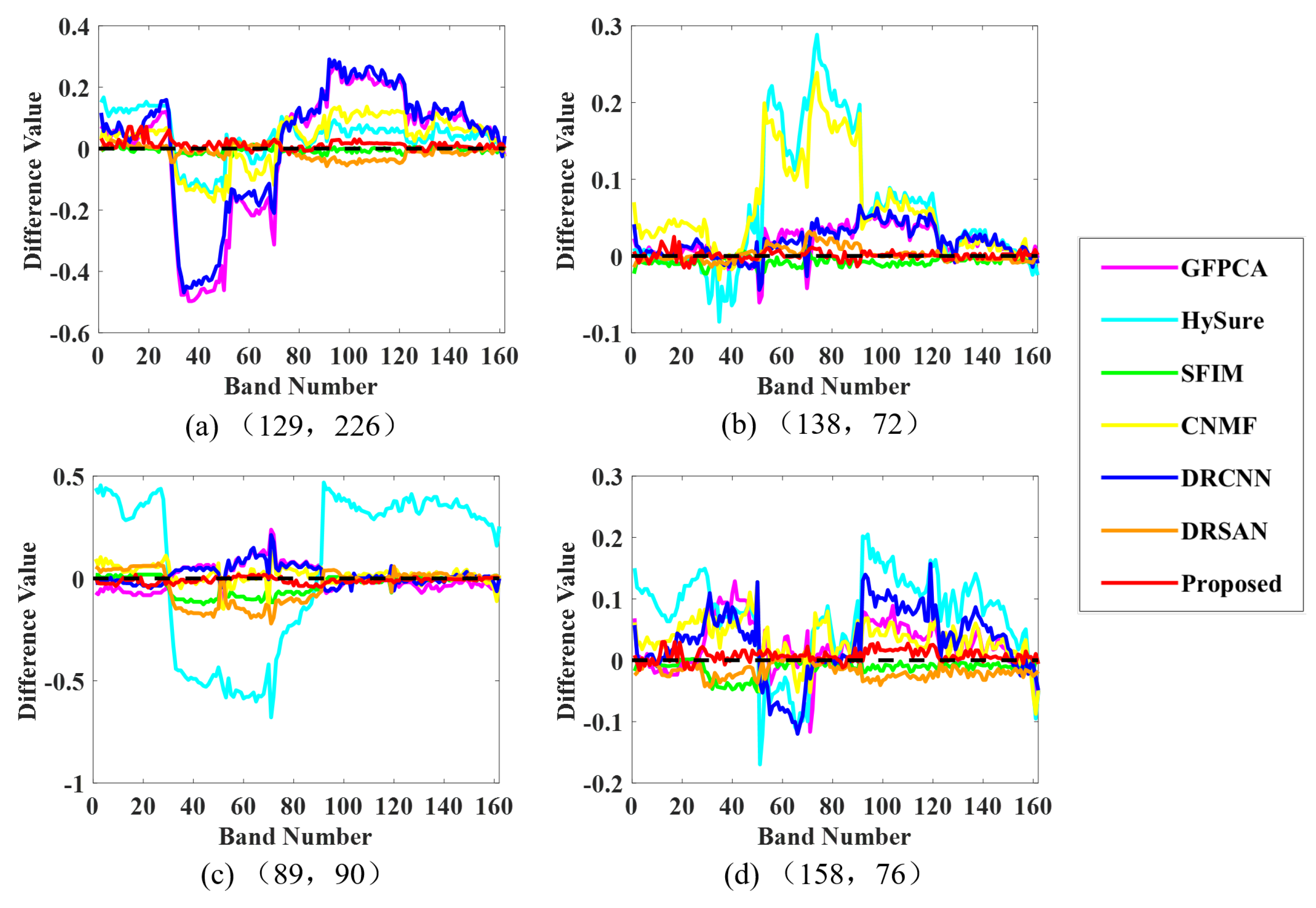
Figure 5 shows the spectral reflectance differences of different methods on the EO-1 dataset compared with the baseline (black dashed line), reflecting the spectral fidelity of the fusion results. Each subplot in the figure represents the spectral reflectance differences at four randomly selected locations for the different fusion methods. The coordinates of the four randomly selected pixels are as follows: (a) (129, 226), (b) (138, 72), (c) (89, 90), and (d) (158, 76). The closer the spectral reflectance difference curve is to the baseline (0), the better the fusion effect. Visually, it is evident that the proposed method exhibits the smallest deviation from the baseline in terms of spectral reflectance difference, indicating the best spectral fidelity of the fused image. The spectral fidelity of SFIM and DRSAN is second best. The spectral reflectance difference curves of other methods fluctuate more, indicating poorer spectral fidelity.

4.5.2. Chikusei Dataset

The pseudo-color fusion results of different fusion methods on the Chikusei dataset are shown in Figure 6. The pseudo-color composite bands are as follows: Red 60, Green 40, and Blue 20. From the figure, it can be seen that methods such as GFPCA, SFIM, and DRCNN exhibit noticeable deviations in both spatial details and color fidelity. However, HySure, CNMF, DRSAN, and the method proposed in this paper show better fusion results in terms of both spatial details and color. Among these, the method proposed in this paper preserves the spatial details most clearly.

Table 4. Evaluation metrics of different fusion methods on the Chikusei dataset.

Method	Q	ERGAS	SAM	CC	RMSE	Time (s)
GFPCA	0.6996	7.7778	5.2997	0.8094	10.4624	0.6142
HySure	0.8001	4.3335	5.2672	0.8256	9.3447	28.1752
SFIM	0.8202	9.6464	4.1682	0.8439	15.1758	0.4894
CNMF	0.8946	6.2779	3.7672	0.9146	8.5365	3.8101
DRCNN	0.7630	8.4678	4.2339	0.8089	19.3449	0.5679
DRSAN	0.8683	4.5246	3.9532	0.8796	8.4892	0.7247
HT	0.8985	4.3310	3.6842	0.9271	7.5032	1.9435
Proposed Method	0.9028	4.1904	3.6381	0.9298	7.3851	0.6534

presents the evaluation metrics of different fusion algorithms on the Chikusei dataset. From the table, it can be seen that the proposed method in this chapter achieves the best results in terms of the Q value and CC value. Additionally, it exhibits the smallest values in ERGAS, SAM, and RMSE, indicating the best performance. Although the running time of the proposed method is not the shortest, it is considered to be at an above-average level compared to other fusion methods. The slightly longer runtime is primarily attributed to the use of two residual spatial attention modules, which enhance feature representation through multiple convolutional operations and dual-scale attention mechanisms (MSA and USA). These modules effectively preserve fine spatial details but introduce additional computational overhead during both training and inference. Furthermore, the ratio transformation stage involves image degradation and refinement processes, which also contribute to the increase in computational complexity.

Figure 7 shows the comparison of spectral reflectance differences between different fusion methods and the baseline (black dashed line) at four randomly selected coordinates on the Chikusei dataset. The coordinates of the randomly selected points are as follows: (a) (42,189), (b) (58,93), (c) (90,147), and (d) (20,149). From the figure, it is visually evident that at the four randomly selected coordinates, the proposed method has the smallest spectral deviation compared to the baseline. HySure shows good spectral preservation at (a), (b), and (d), but exhibits significant fluctuations in some bands at (c). The spectral deviation of the fused image using the SFIM method is the largest.

4.5.3. Impact of Different Parameters on Fusion Results

To investigate the impact of the parameter $\alpha$ on the fusion performance of the proposed method, a detailed statistical analysis was conducted using multiple values of $\alpha$. The experimental results are summarized in

Table 5. Evaluation metrics of different fusion algorithms on EO-1 and Chikusei datasets.

Dataset	$\mathit{\alpha }$	Q	ERGAS	SAM	CC	RMSE
EO-1	0.1	0.4749	7.0828	7.5784	0.8375	8.9346
	0.5	0.8895	5.2749	6.8905	0.9142	7.7804
	0.8	0.9051	5.2682	5.3816	0.9194	7.4982
	0.9	0.9090	5.2104	5.3142	0.9212	7.4123
	1.0	0.9110	5.1973	5.2649	0.9221	7.3834
	1.1	0.9102	5.2156	5.2973	0.9218	7.4078
	1.2	0.9093	5.2984	5.3871	0.9205	7.5210
	5.0	0.7949	6.7854	5.8923	0.8642	9.3585
Chikusei	0.1	0.8234	6.7384	5.9649	0.8197	9.5538
	0.5	0.9011	5.7876	4.8346	0.8879	8.6835
	0.8	0.8988	4.3892	3.8921	0.9252	7.5899
	0.9	0.9019	4.2681	3.6825	0.9280	7.4203
	1.0	0.9028	4.1904	3.6381	0.9298	7.3850
	1.1	0.9005	4.2893	3.7394	0.9271	7.4651
	1.2	0.8977	4.4217	3.8810	0.9243	7.6082
	5.0	0.8532	6.9678	4.0896	0.8563	8.9463

. Initially, four values (0.1, 0.5, 1.0, and 5.0) were selected. Further, additional fine-grained values around 1.0 (i.e., 0.8, 0.9, 1.1, and 1.2) were included to explore the model’s sensitivity near the optimal region.

As shown in the table, when $\alpha =1.0$, the proposed fusion model consistently achieves the best performance on both the EO-1 and Chikusei datasets across multiple evaluation metrics, including Q, ERGAS, SAM, CC, and RMSE. This demonstrates that spatial and spectral loss components contribute equally and synergistically to the final fusion quality. Moreover, the results for nearby values, such as $\alpha =0.9$ and $\alpha =1.1$, are also competitive, suggesting that the model is relatively stable and robust to small changes in this parameter.

5. Discussion

In this paper, we propose a hyperspectral pansharpening method based on ratio transformation and residual networks. Compared with other pansharpening methods, the proposed approach demonstrates superior performance in practical applications. While some existing methods have achieved breakthroughs in specific aspects, they still have notable drawbacks. The GFPCA and SFIM methods exhibit deficiencies in preserving spatial details, failing to effectively restore fine structures in the image. The HySure and CNMF methods perform well in terms of spatial detail preservation but suffer from poor color fidelity, particularly in areas such as lakes, where color distortion is more pronounced. The fusion performance of the DRCNN method is relatively moderate, especially for critical features such as the coastline, where noticeable shape distortion appears in the pseudo-color representation. The DRSAN method performs relatively well in preserving spatial details, but its fused images have lower resolution compared to the proposed method, resulting in inferior detail restoration and spectral fidelity.

Both visually and quantitatively, the proposed method outperforms the comparison methods, achieving superior spectral fidelity and spatial detail retention. Visually, the proposed method distinctly delineates object boundaries, restores finer details, and ensures higher color fidelity, particularly in complex regions such as lakes and mountains. In terms of quantitative evaluation metrics, the proposed method excels in spectral fidelity-related metrics such as the Q and CC values and surpasses other methods in spatial fidelity assessment, demonstrating its ability to enhance image resolution and spectral consistency while preserving image details. The key innovations of the proposed method are as follows:

(1)

The method directly performs fusion on the original images instead of relying on degraded panchromatic and hyperspectral images.

(2)

The initial ratio image, generated through the ratio transformation method, is refined using a residual network to produce a new ratio image, which injects spatial details into the hyperspectral image.

(3)

Spatial-preserving and spectral-preserving loss functions are designed to constrain both spatial and spectral details of the fused image, enabling precise adjustment of the fusion process.

However, the proposed method still has some limitations. First, when processing large-scale or high-resolution images, the computation time may be relatively long, potentially leading to performance bottlenecks in real-time applications. Second, the choice of parameters in the method can significantly influence the final fusion results in different application scenarios. Additionally, when dealing with noisy or low-quality images, the fusion performance may be affected, particularly in high-noise environments where the robustness of the method may be insufficient. To improve inference efficiency and adaptability in future work, three directions are worth exploring: (1) introducing lightweight attention mechanisms such as depthwise separable convolutions or grouped convolutions to reduce parameter count and computational load; (2) applying model compression techniques such as quantization or knowledge distillation to accelerate inference under controllable accuracy loss; and (3) leveraging deployment frameworks like TensorRT or ONNX with mixed-precision inference (e.g., FP16) to fully exploit GPU acceleration and enhance runtime performance in practical applications.

6. Conclusions

In summary, this paper presents a hyperspectral pansharpening method based on ratio transformation and residual networks. By improving three key components—ratio transformation, the residual attention network, and loss functions—we introduce the Ratio Residual Attention Network (RRAN). The experimental results on the EO-1 and Chikusei datasets demonstrate that the proposed method significantly enhances the clarity of spatial details, improves spectral fidelity, and outperforms other comparison methods in terms of fusion effectiveness. We believe that this method holds great potential for a wide range of applications, with significant practical value in fields such as high-resolution remote sensing image processing, environmental monitoring, and disaster assessment.