Sensor-Generated In Situ Data Management for Smart Grids: Dynamic Optimization Driven by Double Deep Q-Network with Prioritized Experience Replay

Abstract

According to forecast data from the State Grid Corporation of China, the number of terminal devices connected to the power grid is expected to reach the scale of 2 billion within the next five years. With the continuous growth in the number and variety of terminal devices in the smart grid, traditional cloud-edge-end architecture will face the increasing issue of response latency. In this context, in situ computing, as a paradigm for local or near-source data processing within cloud-edge-end architecture, is gradually becoming a key technological pathway in industrial systems. The in situ server system, by deploying servers near terminals, enables the near-data-source processing of terminal-generated in situ data, representing an important implementation of in situ computing. To enhance the processing efficiency and response capability of in situ data in smart grid scenarios, this study designs an in situ data processing mechanism and an access demand management framework. Due to the heterogeneity of in situ server performance, there are variations in response capabilities for access demands across rounds. This study introduces a double deep Q-network with prioritized experience replay to assist in response decision-making. Simulation experiments show that the proposed method reduces waiting latency and response latency by an average of 67.69% and 68.77%, respectively, compared to traditional algorithms and other reinforcement learning algorithms, verifying its effectiveness in in situ data management. This scheme can also be widely applied to in situ computing scenarios with low-latency data management, such as smart cities and industrial IoT.

1. Introduction

With the rapid advancement of internet and virtualization technologies, the cloud computing model based on remote servers has swiftly emerged. In 2023, the global cloud computing market reached a scale of USD 586.4 billion and is projected to exceed USD one trillion by 2027. The cloud computing paradigm is gradually replacing the traditional computing model that relies on local hardware resources, demonstrating strong development momentum [1]. According to Gartner’s research, cloud computing can help enterprises reduce IT costs by 30% to 40%. Compared with locally hosted server architectures that require high maintenance costs, cloud-based computing models not only significantly reduce enterprises’ infrastructure investments but also enhance data processing efficiency [2,3]. The rise of cloud computing has provided strong support for data storage, processing, and management in terminal devices, and the Cloud-End System is gradually taking shape.

According to Research and Markets studies, global IoT devices are projected to generate approximately 73.1 zettabytes of data by 2025, nearly a fourfold increase from 18.3 zettabytes in 2019. With the widespread deployment of terminal devices across various industrial systems, the volume of generated data is growing exponentially. However, the traditional approach of uploading massive amounts of data to the cloud for centralized processing is increasingly revealing a range of issues, including bandwidth bottlenecks, transmission latency, and excessive energy consumption [4,5]. To mitigate these challenges, research trends are shifting toward processing data at the network edge, effectively reducing network load, shortening response time, and enhancing overall system processing efficiency [6].

To address these challenges, part of the computing and storage capabilities have been offloaded from centralized cloud servers to network edges closer to terminal devices, leading to the emergence of edge computing [7]. This advancement not only reduces data transmission latency but also enhances the system’s real-time responsiveness and processing efficiency [5]. The Cloud-Edge-End System has been gradually refined, achieving efficient resource utilization and flexible data processing [6].

With the rapid development of the Cloud-Edge-End System, the number of IoT devices is expected to increase from 18.8 billion in 2025 to 40 billion by 2030. Consequently, various terminal devices, sensors, and user behaviors will generate massive volumes of data. In such a distributed scenario, data not only grows explosively in scale but also increases in variety and complexity, posing significant challenges to data storage, scheduling, and processing [8]. The vast amount of data flowing from the device end to the edge and then to the cloud leads to a sharp rise in data transmission frequency and volume, further exacerbating the burden on existing infrastructure [9]. The demand for in situ data processing is gradually emerging.

In the smart grid, the locations of wind turbines are often remote, with factors such as power limitations and other constraints [10]. On the other hand, in the Cloud-Edge-End architecture, edge nodes are primarily deployed in areas with higher demand density [11]. When in situ data relies on the traditional Cloud-Edge-End architecture for storage and access, transmission delays and bandwidth limitations still pose significant challenges. In situ Server (InS) Systems address these limitations by deploying servers directly near the data sources, providing dedicated services to terminal devices with in situ data storage needs, thus forming a comprehensive InS system. Specifically, as shown in

Table 1. Comparison between traditional cloud-edge-end architecture and InS system. This table compares the traditional cloud-edge-end architecture with the InS system across various aspects.

Aspect	Cloud-Edge-End Architecture	InS System
Applicable Scenarios	General-purpose terminals and large-scale application scenarios	Terminal systems requiring in situ data processing
Data Processing	Data is transmitted to remote edge nodes and then uploaded to the cloud	InS performs processing directly near the data source; cloud and edge computing are considered only when necessary
Data Generation Location	Terminal data generated near urban areas	Terminal data generated near wind turbines
End Node Characteristics	Distributed in urban areas with higher computing demand density	Distributed in remote areas due to constraints such as wind conditions and geographic limitations
Edge Nodes Location	Edge nodes are primarily deployed in areas with higher demand density	Edge nodes are primarily deployed in areas with higher demand density
Transmission to Edge Nodes	Relatively short transmission distance	Relatively long transmission distance, significantly constrained by latency and bandwidth limitations

.

In this study, to optimize the in situ data management scheme in the InS system, efficient storage and timely responses are achieved. The specific environment and management architecture are shown in Figure 1. The main contributions of this paper are as follows:

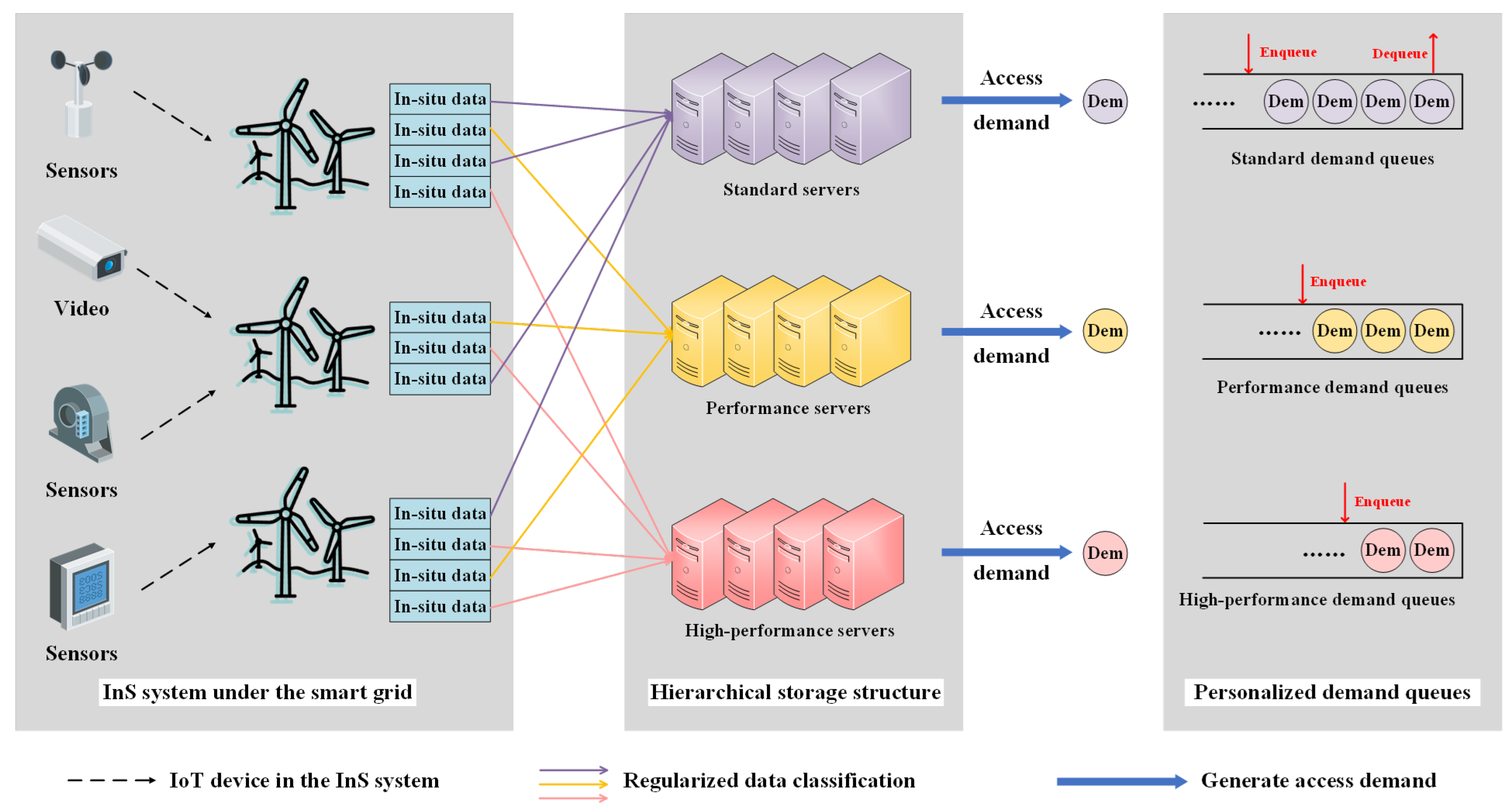
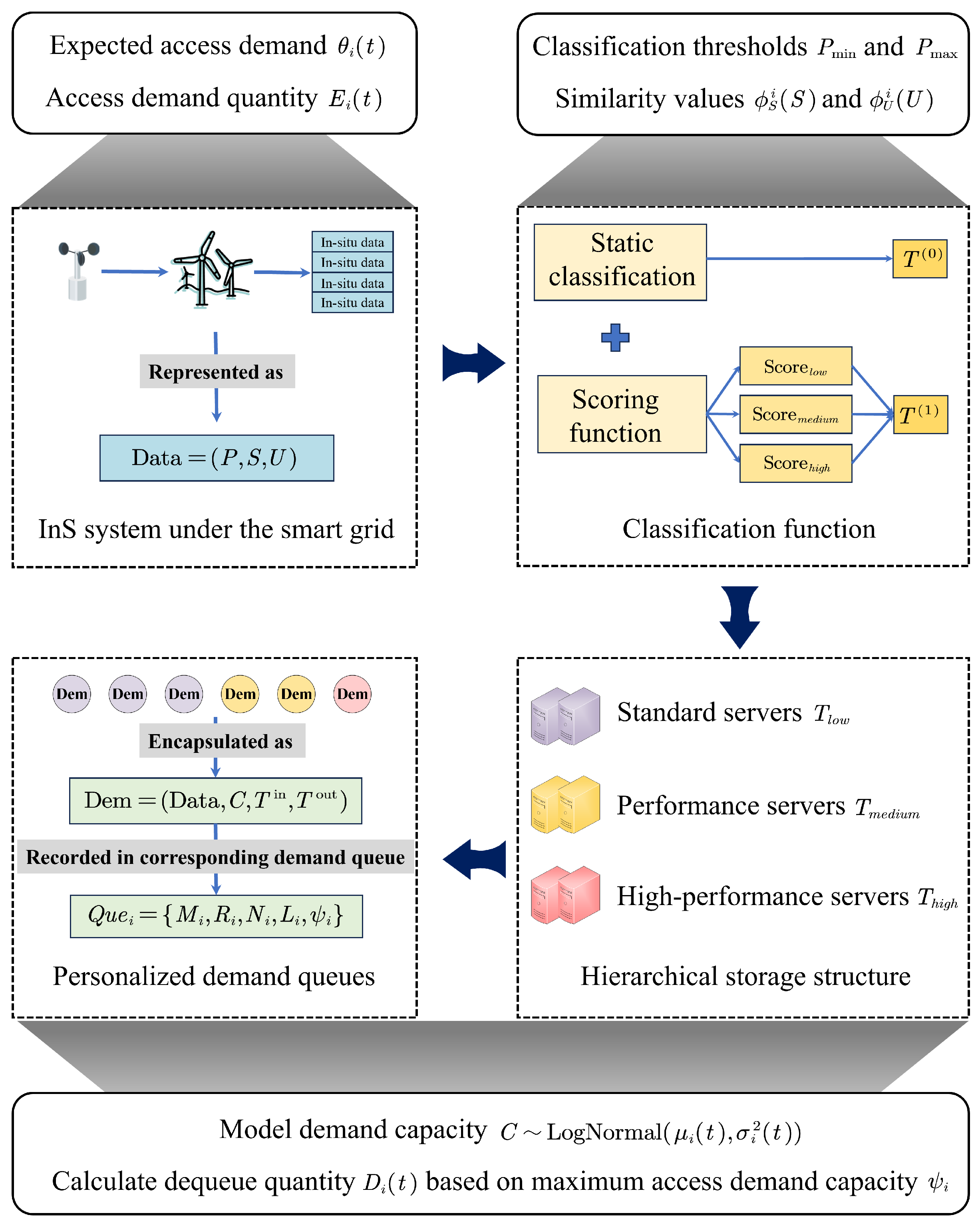
• Design of a hierarchical storage structure: A classification mechanism is designed to preprocess data with different attributes based on the diverse characteristics of in situ data, and store it in server clusters at different hierarchical levels to enhance system access efficiency.
• Design of personalized demand queues: When access demands for in situ data from different hierarchical levels arise, they are received and recorded through personalized demand queues, ensuring timely responses to demands from each level.
• Setting up an algorithm-driven demand response mechanism: For access demands in different personalized demand queues, the Double Deep Q-Network with Prioritized Experience Replay algorithm is introduced to assist in decision-making and response.

Figure 1. InS System and in situ data management architecture. This figure illustrates the architecture of the in situ server system (InS) in a smart grid environment, providing a comprehensive depiction of the overall in situ data management process. It primarily consists of a hierarchical storage structure and personalized demand queues. When terminal devices generate in situ data, the system first classifies the data based on its characteristics and stores it in different server clusters within the hierarchical structure. Subsequently, in response to the generated access demands, the system distributes them into the corresponding queues within the personalized demand queues to support differentiated response strategies.

Figure 1. InS System and in situ data management architecture. This figure illustrates the architecture of the in situ server system (InS) in a smart grid environment, providing a comprehensive depiction of the overall in situ data management process. It primarily consists of a hierarchical storage structure and personalized demand queues. When terminal devices generate in situ data, the system first classifies the data based on its characteristics and stores it in different server clusters within the hierarchical structure. Subsequently, in response to the generated access demands, the system distributes them into the corresponding queues within the personalized demand queues to support differentiated response strategies.

The structure of this paper is as follows: Section 1 introduces the technical background of in situ data management in the InS system within the smart grid. Section 2 discusses the development of smart grid technologies, the application of in situ data and its concepts across multiple domains, and the application of reinforcement learning in the data field. Section 3 introduces the relevant architecture for in situ data management in the InS system and the evaluation metrics for assessing system management schemes. Section 4 presents the DDQN algorithm upon which the management strategy is based. Section 5 details the experimental simulation process and comparative results of the management strategy. Section 6 provides a comprehensive summary of the research.

2. Related Works

2.1. Technological Background of Smart Grid

Smart grids rely on distributed terminal devices to collect multi-source heterogeneous data in real time, including operational parameters such as voltage, current, and power factor, as well as user electricity consumption behaviors and device status data. However, numerous challenges remain at the data management level, particularly concerning real-time performance, security, and data fusion efficiency.

Xiao et al. proposed a multi-source data security protection mechanism based on edge computing to address issues of real-time data processing and secure transmission in smart grids. This mechanism enhances the data processing capability of distributed terminals via an edge computing architecture, reduces transmission latency, improves system response speed, and employs a smart gateway-based data fusion method to achieve integration and secure storage of heterogeneous data [12]. Hong et al. focused on terminal management in the Power IoT and proposed a data acquisition and fusion solution suitable for large-scale devices. They applied distributed computing to perform fusion analysis on data across temporal and spatial dimensions, thereby enhancing data availability and real-time performance [13]. He et al. studied key technologies in information fusion within intelligent distribution systems and proposed an efficient framework for information integration and real-time processing, significantly improving the efficiency of large-scale data analysis and storage [14].

Zeng et al. conducted a systematic literature review to analyze the applications of the Internet of Things (IoT) in the sustainable development of smart cities, with a focus on its roles in smart communities, intelligent transportation, disaster management, and privacy and security. The study reviewed the key attributes of IoT sensors, communication technologies, and data processing methods [15].

In summary, existing research has achieved notable progress in enhancing edge computing capabilities, optimizing data fusion, and securing transmission. However, efficient access and management of in situ data remain insufficiently explored. This paper aims to further reduce system latency and improve overall operational efficiency by optimizing the access mechanism of distributed terminal in situ data, offering new perspectives for efficient data management in smart grids.

2.2. Related Research on In Situ Data

In situ data and its underlying concept have been widely applied across various domains, including high-performance computing and distributed systems.

Li et al. proposed the In situ Server System, which brings computing resources closer to data sources to preprocess part or all of the in situ data, thereby accelerating data response and storage efficiency [16]. Cisco introduced the concept of fog computing, leveraging devices near data sources (such as routers) to directly process in situ data, aiming to reduce dependence on the cloud. Although this approach has achieved certain success in alleviating network traffic, its focus remains on network optimization, and the computational capabilities and applicability of in situ computing are still relatively limited [17]. In the field of high-performance computing (HPC), large-scale compute-intensive tasks are common, particularly in scientific simulations and big data analysis. These scenarios often involve massive datasets requiring complex computations within limited timeframes. To reduce I/O overhead and enhance processing efficiency, the concept of in situ computing has been introduced to efficiently process large-scale data without incurring additional transmission costs [18,19].

In summary, existing research demonstrates the significant value of in situ computing and its concepts in various fields, particularly in improving data processing efficiency and reducing system burden. However, for distributed terminal data in smart grid scenarios, systematic studies on efficient in situ data storage and management remain lacking. Based on the InS system architecture, this paper proposes an in situ data management method for smart grids, aiming to optimize data access efficiency at the terminal side, reduce overall system latency, and further promote the intelligent evolution of smart grid data management.

2.3. Reinforcement Learning in Data Management

Reinforcement learning, as a data-driven learning method, offers significant advantages over traditional techniques, not only due to its adaptability but also because it continuously optimizes strategies through ongoing feedback mechanisms. By guiding the system to gradually find optimal solutions through reward and punishment signals, reinforcement learning improves scheduling optimization efficiency over time. Reinforcement learning has also achieved numerous research outcomes in the field of data management.

Park et al. proposed a hierarchical storage system for Neural Processing Units (NPU), TM-Training, which optimizes data storage strategies using reinforcement learning. By analyzing data access patterns, reinforcement learning adaptively allocates storage resources at different levels to improve storage efficiency [20]. Anjum et al. studied how reinforcement learning can be used to optimize the security of medical data storage in IoT environments, optimizing data access strategies to enhance security and privacy protection [21]. Guan et al. proposed a data storage optimization method for cloud computing environments, dynamically adjusting data storage strategies through reinforcement learning to reduce redundant data storage and improve storage utilization [22]. Yuan et al. explored the application of reinforcement learning in smart grid data management, proposing a reinforcement learning algorithm based on edge computing to optimize the storage management of multi-source heterogeneous data in smart grids, and enhancing grid stability through real-time data analysis [23]. Zielosko et al. proposed a method for intelligent storage tier management using reinforcement learning, optimizing data allocation in storage systems to improve data retrieval efficiency [24].

In summary, existing research demonstrates that reinforcement learning has played a critical role in multiple fields, particularly in data management across various network architectures and edge environments, providing effective solutions to enhance network performance, reduce energy consumption, and improve security. However, the efficient management of in situ data remains an area requiring further research. This paper combines the characteristics of smart grids to propose a reinforcement learning-driven in situ data management method, aiming to further improve the access efficiency and system performance of in situ data in smart grids.

2.4. In Situ Data Storage Management

The storage method of in situ data is closely related to the functionality of data-generating devices, data volume, processing requirements, and storage durability demands [25]. In edge computing architectures, the servers used for storage are particularly critical, as they directly affect storage efficiency, access speed, and data persistence. Selecting appropriate servers based on different application requirements and device capabilities ensures that data can be effectively stored, accessed rapidly, and retained over long periods.

Traditional in situ data storage typically relies on a single server without detailed differentiation based on specific storage requirements of in situ data. The advantage of this approach lies in its relatively simple system architecture and fixed cost, making it suitable for scenarios with stable data volumes and low processing demands. However, this method also exhibits several limitations, such as low storage space utilization, slower response speeds, and difficulties in handling diverse data types and scales [26].

In summary, existing in situ data storage methods can effectively improve storage efficiency and access speed in certain scenarios, but still face numerous challenges when dealing with complex data of various types and scales. Further research is needed to achieve more flexible and efficient in situ data storage in complex environments such as smart grids.

3. System Modeling

This section provides a detailed description of the system modeling process, including the Hierarchical Storage Structure, Personalized Demand Queues, and system optimization metrics. The complete modeling workflow is illustrated in Figure 2.

3.1. Hierarchical Storage Structure

In traditional power grids, a single medium is often used to store in situ data, whether it is sensor data, equipment operation information, maintenance records, or various types, sizes, and update frequencies of data, all stored in the same medium. As the volume of data continues to grow, not only will the access costs increase, but storage efficiency and read speeds will gradually decrease, leading to slower data access and potentially affecting real-time data processing and decision-making.

In the InS scenario, in situ data exhibits diverse types and rapid growth in scale. Traditional architectures struggle to allocate storage resources efficiently according to actual storage demands, resulting in suboptimal storage efficiency. Considering the heterogeneity of in situ data generated by distributed devices, this study focuses on three key storage features: static priority P, storage size S, and update frequency U. Each piece of in situ data can be represented in the form of a triplet:

$$\mathrm{Data}=(P,S,U)$$

(1)

where the static priority P distinguishes the priority of the in situ data and takes an integer value between 1 and 10. The storage size S indicates the current storage size of the in situ data and is a positive real number. The update frequency U represents the update frequency of the in situ data and is also a positive real number.

According to the static priority P of each in situ data item, the data is preliminarily assigned to three types of servers with different performance levels. Two classification thresholds, $P_{\min }$ and $P_{\max }$, are derived from historical data analysis to reflect the actual demands associated with different priority levels. Data with priority values below $P_{\min }$ is preliminarily classified to the standard-performance server $T_{\mathrm{low}}$, those within the intermediate range are assigned to the medium-performance server $T_{\mathrm{medium}}$, and high-priority data with values greater than or equal to $P_{\max }$ is assigned to the high-performance server $T_{\mathrm{high}}$.

$$T^{\left(0\right)}=\left\{\begin{array}{cc}{T}_{low},\hfill & P<P_{\min }\hfill \\ T_{medium},\hfill & P_{\min }\le P<P_{\max }\hfill \\ T_{high},\hfill & P\ge P_{\max }\hfill \end{array}\right.$$

(2)

Based on static priority classification, this study further introduces two key features of the data to refine and adjust the preliminary classification results. i denotes the specific category of servers, which can take values $low$, $medium$, or $high$. The system evaluates the overall matching degree between each piece of in situ data and the i-type server using a weighted similarity function. The scoring function considers two dimensions: storage size and update frequency, with the weights ${\omega }_S$ and ${\omega }_U$ controlling their relative importance in the total score. A higher score indicates that the data is more suitable, in terms of characteristics, to be assigned to the i-type server. The similarity-based classification result is denoted as $T^{\left(1\right)}$:

$${\mathrm{Score}}_i={\omega }_S·{\varphi }_S^i\left(S\right)+{\omega }_U·{\varphi }_U^i\left(U\right)$$

(3)

$$T^{\left(1\right)}=arg\underset{i}{max}{\mathrm{Score}}_i,i\in \{low,medium,high\}$$

(4)

where ${\varphi }_S^i\left(S\right)$ and ${\varphi }_U^i\left(U\right)$ respectively represent the similarity values calculated using Gaussian functions for the storage size S and update frequency U of the current data, measuring the degree of matching with the expected service characteristics of the i-type server category. The calculation is as follows:

$${\varphi }_S^i\left(S\right)=exp\left(-{\displaystyle \frac{{(S-{\mu }_S^i)}^2}{2{\sigma }_S^2}}\right),{\varphi }_U^i\left(U\right)=exp\left(-{\displaystyle \frac{{(U-{\mu }_U^i)}^2}{2{\sigma }_U^2}}\right),i\in \{low,medium,high\}$$

(5)

where ${\mu }_S^i$ and ${\mu }_U^i$ denote the average values of storage size and update frequency for the i-type server category based on historical data, while ${\sigma }_S$ and ${\sigma }_U$ are the standard deviations obtained from global historical data, reflecting the dispersion of overall data characteristics. The standard deviation serves as a measure of deviation from the expected feature values, facilitating a more accurate characterization of the data’s suitability for each server category, thereby enhancing the precision and robustness of classification decisions.

The system ultimately performs a dynamic adjustment to the initial priority classification results based on the similarity scores. The decision logic for the classification process is expressed as follows:

$$T=\left\{\begin{array}{cc}{T}^{\left(1\right)},\hfill & \mathrm{if}{T}^{\left(1\right)}\ne T^{\left(0\right)}\mathrm{and}\left|{\mathrm{Score}}_{T^{\left(1\right)}}-{\mathrm{Score}}_{T^{\left(0\right)}}\right|>\epsilon \hfill \\ T^{\left(0\right)},\hfill & \mathrm{otherwise}\hfill \end{array}\right.$$

(6)

First, the initial classification result $T^{\left(0\right)}$ is obtained according to the static priority information. Then, the similarity scores of the data under each server category are computed, and the category with the highest score is selected as the adjusted classification $T^{\left(1\right)}$. If $T^{\left(0\right)}$ and $T^{\left(1\right)}$ are inconsistent and the score difference between them exceeds a threshold $\epsilon$, it indicates a significant deviation between the service-level characteristics of the current in situ data and the initial judgment. In this case, the system adopts $T^{\left(1\right)}$ as the final classification result; otherwise, the initial allocation is retained.

3.2. Personalized Demand Queues

In the InS system, in situ data is stored in servers with matching performance. Subsequently, different servers will generate data access demands continuously. However, there is a disparity in the update frequencies of the in situ data across different servers, which leads to differences in the volume of generated data access demands. To better ensure response speed, this study designs personalized demand queues to receive data access demands: each type of server’s data access demands are recorded with the round count in the corresponding demand queue. Each demand queue $Qu{e}_i$ can be represented as follows:

$$Qu{e}_i=\{M_i,R_i,N_i,L_i,{\psi }_i\},i\in \{low,medium,high\}$$

(7)

where the queue $Qu{e}_i$ is used to receive access requests for in situ data generated by server $T_i$. To characterize the properties of the queue, this study introduces the following key variables: $M_i$ denotes the maximum request capacity of the queue; $R_i$ represents the current remaining available capacity, which is a positive integer constrained by the server’s own performance. $N_i$ records the number of access demands that have already been served in the queue, and $L_i$ denotes the cumulative delay generated by all completed access demands in the queue; both are positive integers. ${\psi }_i$ indicates the maximum number of access demands the queue can process in a single time step when it is selected, also a positive integer, reflecting the server’s processing capability. $|Qu{e}_i|$ denotes the current number of access demands in the queue.

The access demands generated by different servers are recorded with the number of rounds in the corresponding queue $Qu{e}_i$. The scheduling demand can be expressed as follows:

$$\mathrm{Dem}=\{\mathrm{Data},C,T^{\mathrm{in}},T^{\mathrm{out}}\}$$

(8)

where C represents the occupied demand queue capacity. $T^{\mathrm{in}}$ is the enqueue round of the access demand, initialized as the current round number $T^{now}$. $T^{\mathrm{out}}$ is the dequeue round of the access demand, initialized as empty, and when it is responded to, it will be set to the current round number $T^{now}$.

3.3. Evaluation Metrics

To objectively and comprehensively evaluate in situ data management schemes driven by different algorithms, this study simulates the in situ data access management environment under the InS system. To comprehensively assess the proposed in situ data management mechanism, three metrics are selected: Average Waiting Delay (AWD), Average Residual Requirements (ARR), and Average Response Latency (ARL). These metrics respectively quantify system performance from the perspectives of response capability, queue congestion, and the processing efficiency of completed requests, thereby providing a comprehensive reflection of the data management strategy in terms of real-time performance and load balancing.

3.3.1. Average Waiting Delay

$AWD$ is used to measure the average number of waiting rounds from the entry to the current round for unresponsive demands in the system during each round. This metric reflects the timeliness of the system in handling requests and reveals the effectiveness of the management strategy in optimizing queue responses.

Independently calculate the average waiting delay $AW{D}_i$ for each queue. First, traverse all unresponsive demands in queue $Qu{e}_i$ and calculate the difference between the entry round $T^{in}$ and the current round $T^{now}$ for each demand, thus obtaining the waiting delay for each demand. Then, accumulate the waiting time of all unresponsive demands to obtain the total waiting time for queue $Qu{e}_i$ in that round. Finally, divide the total waiting time by the number of demands to obtain the average waiting delay $AW{D}_i$ of queue $Qu{e}_i$ in that round.

$$AW{D}_i={\displaystyle \frac{1}{|Qu{e}_i|}}\sum _{\mathrm{Dem}\in Qu{e}_i}(T^{now}-T^{in}),i\in \{low,medium,high\}$$

(9)

The system’s average waiting delay $AWD$ is the average of each queue’s $AW{D}_i$.

$$AWD={\displaystyle \frac{1}{3}}\sum AW{D}_i,i\in \{low,medium,high\}$$

(10)

$AWD$ dynamically tracks the enqueue time of demands to quantify the system’s waiting time within a specific round. By analyzing the status of each queue $Qu{e}_i$, the effectiveness of the in situ data management strategy can be evaluated, providing an optimization basis for subsequent queue responses. A smaller $AWD$ value indicates that the management strategy effectively considers the waiting delay across all queues in the system. An effective strategy can reduce $AWD$ by optimizing queue selection, minimizing the number of waiting rounds for demands, and enhancing the overall system responsiveness.

3.3.2. Average Residual Requirements

$ARR$ is used to measure the residual quantity of unresponded access demands in the system. It reflects the system’s real-time processing capability and load management status, serving as a key metric for evaluating task backlog, system load, and response timeliness.

The number of unresponded demands $|Qu{e}_i|$ in each queue is counted for the current round, and the residual demand $AR{R}_i$ is calculated independently for each queue. The system’s average residual requirements $ARR$ is defined as the average of all $AR{R}_i$ values:

$$AR{R}_i=|Qu{e}_i|,ARR={\displaystyle \frac{1}{3}}\sum \left|Qu{e}_i\right|,i\in \{low,medium,high\}$$

(11)

$ARR$ quantifies the system load and task backlog by counting unresponded demands across all queues, aiding in the evaluation of scheduling strategies under high-concurrency scenarios. Variations in $AR{R}_i$ among different queues can also provide optimization insights for in situ data management strategies. A smaller $ARR$ indicates that the system effectively accounts for demand accumulation across queues, ensuring timely responses to most demands and enhancing overall system performance and reliability.

3.3.3. Average Response Latency

$ARL$ is used to measure the average number of rounds experienced by responded access demands from enqueuing to dequeuing in each round. This metric is crucial for evaluating the system’s response efficiency and timeliness assurance capability.

The average response latency $AR{L}_i$ is calculated independently for each queue. In each round, both the number of responded demands $N_i$ and the accumulated response latency $L_i$ in queue $Qu{e}_i$ are updated. The average response latency for queue $Qu{e}_i$ in the current round is obtained by computing the ratio of these two parameters.

$$AR{L}_i={\displaystyle \frac{L_i}{N_i}},i\in \{low,medium,high\}$$

(12)

The system’s average response latency $ARL$ is defined as the average of all $AR{L}_i$ values:

$$ARL={\displaystyle \frac{1}{3}}\sum AR{L}_i,i\in \{low,medium,high\}$$

(13)

$ARL$, by accumulating the response delay of completed tasks in each queue, reflects the system’s dynamic response capability and the effectiveness of response strategies under varying loads. The differences in $AR{L}_i$ across queues provide a perspective to evaluate in situ data management strategies from the viewpoint of cumulative latency, which facilitates strategy adjustment based on feedback from completed demands. A smaller $ARL$ indicates higher efficiency in task response and slower delay accumulation, thereby enhancing overall response rate and system performance.

Under the static consideration of server performance limitations per round, the above three evaluation metrics quantitatively analyze the performance of data management strategies from the two core dimensions of system latency and demand response rate. This provides a comprehensive reflection of the optimization capabilities of different algorithms in ensuring real-time performance and load control.

4. Algorithm

4.1. Demand Enqueue Rules

To more realistically simulate the temporal correlation and load fluctuation of in situ data, the system caches the amount of access demand E generated in the most recent w rounds and dynamically updates it as the rounds progress. To better simulate the demand generation process, the expected access demand $\theta \left(t\right)$ in round t is computed using an Exponentially Weighted Moving Average (EMA) over the historical demand data from the previous w rounds. The calculation is given by the following:

$$\theta \left(t\right)=\sum _{k=1}^w{\beta }_k·E(t-k),\sum _{k=1}^w{\beta }_k=1,{\beta }_1>{\beta }_2>\cdots >{\beta }_w$$

(14)

where ${\beta }_k$ denotes the weight assigned to the k-th historical value, which decays exponentially, and the total weight sums to 1. The EMA model assigns higher weights to more recent data, thereby effectively capturing short-term fluctuations in the system, making it well-suited for the rapidly changing access demand characteristics in in situ (InS) scenarios.

To more realistically simulate the fluctuating generation process of access demand, this study adopts a Poisson distribution to model the number of access demands generated by the system. The number of demands enqueued at episode t, denoted as $E\left(t\right)$, can be expressed as follows:

$$E\left(t\right)\sim \mathrm{Poisson}\left(\lambda \right(t\left)\right),\lambda \left(t\right)=\zeta ·\theta \left(t\right),i\in \{low,medium,high\}$$

(15)

where $\lambda \left(t\right)$ denotes the mean of the Poisson distribution. The adjustment factor $\zeta$ is used to control the scaling of the Poisson distribution, with a value range of $\zeta \in [1.0,1.5]$. This range effectively captures the load fluctuations typical of in situ (InS) systems under both normal and moderately peaked conditions. Once the total access demand for each round is determined, a classification mechanism is applied to assign the specific number of access demands entering each queue $Qu{e}_i$ in round t: $E_{low}\left(t\right)$, $E_{medium}\left(t\right)$, and $E_{high}\left(t\right)$.

In practice, the required capacity of access demands is unevenly distributed, with a small number of large-capacity and a majority of small-capacity demands, which aligns with the characteristics of a log-normal distribution. $E_i\left(k\right)$ denotes the number of access demands enqueued in queue $Qu{e}_i$ at round k. $C_i^{(k,j)}$ represents the required capacity of the j-th access demand in queue $Qu{e}_i$ at round k, where $j=1,2,\dots ,E_i\left(k\right)$. ${\mathcal{H}}_i\left(t\right)$ is a set that records the required capacities of all access demands in queue $Qu{e}_i$ during the w rounds preceding round t. It is formally defined as follows:

$${\mathcal{C}}_i^{\left(k\right)}=\{C_i^{(k,1)},C_i^{(k,2)},\dots ,C_i^{(k,E_i\left(k\right))}\},i\in \{low,medium,high\},k\in [t-w,t-1]$$

(16)

$${\mathcal{H}}_i\left(t\right)=\bigcup _{k=t-w}^{t-1}{\mathcal{C}}_i^{\left(k\right)},i\in \{low,medium,high\}$$

(17)

Subsequently, based on maximum likelihood estimation, two key parameters of the log-normal distribution followed by each queue in round t are estimated: the mean ${\mu }_i\left(t\right)$ and the variance ${\sigma }_i^2\left(t\right)$. Sampling is then performed to generate the required capacity C of each access demand in the current round t.

$${\mu }_i\left(t\right)={\displaystyle \frac{1}{|{\mathcal{H}}_i\left(t\right)|}}\sum _{C_j\in {\mathcal{H}}_i\left(t\right)}log{C}_j,i\in \{low,medium,high\}$$

(18)

$${\sigma }_i^2\left(t\right)={\displaystyle \frac{1}{|{\mathcal{H}}_i\left(t\right)|}}\sum _{C_j\in {\mathcal{H}}_i\left(t\right)}{\left(\log C_j-{\mu }_i\left(t\right)\right)}^2,i\in \{low,medium,high\}$$

(19)

$$C\sim \mathrm{LogNormal}({\mu }_i\left(t\right),{\sigma }_i^2\left(t\right))$$

(20)

The Poisson distribution is not only a typical model for describing data generation in industrial scenarios, but also more accurately reflects the actual generation efficiency of in situ data access demand. The log-normal distribution, through effective analysis of historical data, can accurately simulate the volatility of demand capacity, ensuring that the required capacity better aligns with the asymmetric characteristics in real-world scenarios. Ultimately, the access demand generated by each queue must satisfy the following constraints:

$$\sum _1^{E_i\left(t\right)}C\le R_i\le M_i,i\in \{low,medium,high\}$$

(21)

The remaining demand capacity $R_i$ of the queue must always be less than or equal to the maximum demand capacity $M_i$ of the queue. Only when the actual number of generated scheduling demands satisfies the above constraint can the generated demands be loaded into the corresponding demand queue $Qu{e}_i$; otherwise, the generated demand is retained and will be loaded into the demand queue once the condition is met. The specific enqueuing process is shown in Algorithm 1.

Algorithm 1 Demand Enqueue Rules

Parameters: Expected access demand ${\theta }_i\left(t\right)$, adjustment factor $\zeta$, maximum request capacity $M_i$, remaining available capacity $R_i$  1: Initialize demand queues $Qu{e}_i$,   $i\in \{low,medium,high\}$;  2: Initialize ${\theta }_i\left(t\right)$ for each queue $Qu{e}_i$;  3: Initialize $\zeta$ as an adjustment factor to regulate demand generation rate;  4: Compute the mean of the Poisson distribution ${\lambda }_i\left(t\right)=\zeta ·{\theta }_i\left(t\right)$;  5: for each round do  6:      for each queue $Qu{e}_i$ do  7:          Generate demand quantity $E_i\left(t\right)\sim \mathrm{Poisson}\left({\lambda }_i\left(t\right)\right)$;  8:          if ${\sum }_1^{E_i\left(t\right)}C\le R_i\le M_i$ then  9:               for each generated demand $\mathrm{Dem}$ do 10:                   Set enqueue round: $T^{\mathrm{in}}=T^{now}$; 11:                   Set dequeue round: $T^{\mathrm{out}}=\varnothing$; 12:                   Enqueue the demand into $Qu{e}_i$; 13:              end for 14:              Update remaining available capacity of $Qu{e}_i$: $R_i-={\sum }_1^{E_i\left(t\right)}C$ 15:         else 16:              Retain generated demand until condition is met; 17:         end if 18:      end for 19: end for

4.2. Demand Dequeue Rules

Due to the differences in server performance, the speed at which they process access demands varies. The system constraint requires that each access demand be fully processed within a single round, without spanning across rounds or being split. Therefore, in round t, the system will traverse the front of the queue $Qu{e}_i$ and calculate the number of access demands $D_i\left(t\right)$ that can be processed within this round, provided that the queue is selected for scheduling.

When the algorithm selects queue $Qu{e}_i$, based on the maximum access demand capacity ${\psi }_i$ that can be processed in a single round and the self-generated capacity C of the demand at the front of the queue, the number of access demands that can be processed in the current round when each queue is selected can be calculated as follows:

$$D_i\left(t\right)=max\left\{n\in {\mathbb{N}}^{+}\right.\left|\sum _{k=1}^n{C}_k\le {\psi }_i\right\},i\in \{low,medium,high\}$$

(22)

When the selected queue $Qu{e}_i$ is chosen to respond, the access demands at the front of the queue need to be processed in a first-come, first-served manner, with a specified number of demands being dequeued sequentially and the parameter $N_i$ being updated. Each access demand that is executed in response needs to accumulate delay in the parameter $L_i$, and the specific calculation formula is as follows:

$$L_i=\sum _1^{D_i\left(t\right)}{T}^{out}-T^{in}$$

(23)

In each round, all queues perform the enqueue operation. However, differences exist in the response capabilities of each queue. This study aims to comprehensively consider queue congestion and access demand latency across the entire system, selecting one queue per round for response. This not only ensures the access rate but also effectively mitigates system latency. The specific dequeue process is shown in Algorithm 2.

Algorithm 2 Demand Dequeue Rules

Parameters: Dequeued quantity $D_i\left(t\right)$, number of responded access demands $N_i$, cumulative delay caused by responded access demands $L_i$  1: Initialize $L_i=0$ for all queues;  2: Initialize $N_i=0$ for all queues;  3: for each round do  4:     Select a queue $Qu{e}_i$ based on system;  5:     Initialize $count=0$;  6:     while $count<D_i\left(t\right)$ and $Qu{e}_i$ is not empty do  7:         Dequeue a demand $\mathrm{Dem}$ from the head of $Qu{e}_i$;  8:         Set dequeue round: $T^{out}=T^{now}$;  9:         Compute response delay: $L_i\leftarrow L_i+(T^{out}-T^{in})$; 10:        Update the number of responded access demands: $N_i\leftarrow N_i+1$; 11:        $count\leftarrow count+1$; 12:        Update remaining available capacity of $Qu{e}_i$: $R_i-=C$ 13:     end while 14: end for

4.3. Markov Modeling

The state represents the characteristics or information of the environment at a certain moment. The state determines the observations of the agent and influences future decisions and rewards. In the process of in situ data management in the InS system, the state at each time step t consists of three current system evaluation metrics: $AWD$, $ARR$, and $ARL$. These metrics comprehensively characterize the service performance of the InS system at each time step.

However, since the original values of these three indicators are real numbers with unfixed upper and lower bounds, directly using them in reinforcement learning would result in an infinite state space, which prevents the convergence of the Q-learning algorithm. To control the value range of the evaluation indicators without affecting their relative differences, the three system-level evaluation indicators are normalized as follows:

$$x^{\mathrm{norm}}={\displaystyle \frac{x}{1+x}},x\in \{AWD,ARR,ARL\}$$

(24)

where x denotes the original indicator value and $x^{\mathrm{norm}}$ represents the normalized value. After normalization, in order to discretize the state space for Q-learning, each normalized indicator value is further divided into n (default is 5) fixed intervals and mapped to discrete integers. The discretization process is defined as follows:

$$x^{\mathrm{disc}}=⌊n·x^{\mathrm{norm}}⌋,x^{\mathrm{norm}}\in \left(0,1\right)$$

(25)

After normalization and discretization, the system state is ultimately represented as a three-dimensional discrete vector. Each dimension takes values from a finite set, effectively transforming the originally continuous state space into a finite discrete state space, which provides theoretical support for the stability and convergence of subsequent algorithm training. $s_t$ denotes the state at time step t, and $\mathcal{S}$ denotes the finite discrete state space, defined as follows:

$$s_t=\left[\begin{array}{c}AW{D}^{\mathrm{disc}},AR{R}^{\mathrm{disc}},AR{L}^{\mathrm{disc}}\end{array}\right]\in \mathcal{S}$$

(26)

The action represents the decision made by the agent in a specific state, determined by the policy function $\pi$, and directly affects the next state of the environment and the reward received. In the process of in situ data management, $a_t$ denotes the action selected at time step t, i.e., the target access demand queue responded to in the current round. $\mathcal{A}$ denotes the prioritized discrete action space, which can be represented as follows:

$$a_t\in \mathcal{A}=\{Qu{e}_{low},Qu{e}_{medium},Qu{e}_{high}\}$$

(27)

The reward represents the feedback signal received by the agent after executing a certain action, serving as a measure of the decision’s effectiveness. The agent’s objective is to maximize the cumulative reward. To ensure the stability of the reward function during the training process and to satisfy the boundedness assumption required by Q-learning, the reward function $R(s_t,a_t)$ at time step t is composed of three normalized system metrics:

$$R(s_t,a_t)=-\left(AW{D}^{\mathrm{norm}}+AR{R}^{\mathrm{norm}}+AR{L}^{\mathrm{norm}}\right)$$

(28)

The policy $\pi$ defines the rules or strategy by which the agent selects an action in each state. The policy can be defined as a function $\pi \left(s\right)$ mapping state $s_t$ to action a, which can be specifically expressed as follows:

$$\pi \left(s_t\right)=a_t$$

(29)

In summary, although the system state at each time step is derived from real-time system metrics rather than based on an explicit state transition probability function, the management process of access demand for in situ data in the InS system can still be formalized as a Markov Decision Process (MDP) that satisfies the Markov property, defined as follows:

$$\mathcal{M}=(\mathcal{S},\mathcal{A},R,\gamma )$$

(30)

where the discount factor $\gamma$ is used to balance the trade-off between immediate and future rewards. In MDP modeling, the policy is optimized through reinforcement learning algorithms to maximize the cumulative reward.

4.4. Double Deep Q-Network with Prioritized Experience Replay

In the in situ data management process, the agent often needs to undergo multiple interactions before receiving effective rewards related to its decisions, resulting in low training efficiency for traditional Q-learning in environments with delayed rewards. To address this issue, this study introduces the Double Deep Q-Network with Prioritized Experience Replay (DDQN-PER) algorithm for decision optimization of personalized access demand queues. The core idea is to gradually learn the optimal queue selection policy through continuous interaction with the entire system environment. Figure 3 illustrates the complete process and framework structure of the DDQN-PER algorithm. This study integrates the Double DQN mechanism proposed by Van Hasselt et al. [27] and the Prioritized Experience Replay (PER) method introduced by Schaul et al. [28]. The following section begins with a detailed description of the algorithm’s computational process.

At each decision moment t, the agent perceives the current system state $s_t$ and, based on the current Q-Network, selects the action $a_t$ to execute. This process follows the $ϵ$-greedy policy, where with a certain probability $ϵ$, a random action is chosen, and the action with the highest Q-value is selected for the remaining time:

$$a_t=\left\{\begin{array}{cc}\mathrm{random}\mathrm{action},\hfill & \mathrm{with}\mathrm{probability}ϵ\hfill \\ arg\underset{a}{max}Q(s_t,a;\theta ),\hfill & \mathrm{otherwise}\hfill \end{array}\right.$$

(31)

The agent applies the action $a_t$ to the environment, and the environment returns the immediate reward $r_t$ and the next state $s_{t+1}$. These interaction data $(s_t,a_t,r_t,s_{t+1})$ are stored in the experience replay buffer (Replay Memory) for subsequent training. Even if the rewards of certain decisions are manifested after multiple steps, the associated experiences can still be repeatedly sampled, thereby enhancing the learning of delayed rewards. The introduced Prioritized Experience Replay mechanism not only requires storing experiences in the buffer but also calculating the TD error ${\delta }_t$ for each experience:

$${\delta }_t=y_t-Q(s_t,a_t;\theta )$$

(32)

In addition, the Prioritized Experience Replay mechanism calculates the priority $p_i$ for each experience based on the Temporal Difference error (TD error). The TD error reflects the impact of the current experience on Q-Network training, and thus, through priority-weighted sampling, the agent learns more from experiences with larger errors. The priority $p_i$ can be expressed as follows:

$$p_i=\left|{\delta }_t\right|+ϵ$$

(33)

where $ϵ$ is a small constant used to avoid the situation where the priority is zero. This mechanism is well-suited to scenarios with delayed rewards, as such experiences are more likely to yield larger TD errors in the future, thereby being assigned higher priorities and sampled more frequently during training.

During training of the DDQN-PER model, the Prioritized Experience Replay mechanism performs weighted random sampling from the experience replay buffer, based on the priority of each experience $(s_t,a_t,r_t,s_{t+1})$. Experiences with higher priorities are more likely to be sampled. The sampling probability $P\left(i\right)$ is computed based on the priority $p_i$ of each experience, and $\alpha$ controls the bias in the prioritized sampling:

$$P\left(i\right)={\displaystyle \frac{p_i^{\alpha }}{{\sum }_k{p}_k^{\alpha }}}$$

(34)

After sampling a batch of data from the replay buffer, the next step is to calculate the importance sampling weight ${\omega }_i$ for each sampled experience, which is calculated as follows:

$${\omega }_i={\left({\displaystyle \frac{1}{N}}·{\displaystyle \frac{1}{P\left(i\right)}}\right)}^{\beta }$$

(35)

where N denotes the size of the replay buffer, which also represents the total number of experiences in the experience pool. $P\left(i\right)$ is the probability of the current experience being sampled. $\beta$ is the parameter that controls the bias of the importance sampling weights.

Unlike DQN, which directly utilizes the Target Q-Network to both select and evaluate the optimal action, DDQN introduces a dual-network structure, where separate networks are employed for action selection and action evaluation. This mechanism not only effectively alleviates the overestimation of Q-values but also allows the agent to learn action values more stably in the presence of delayed rewards. In practice, DDQN first selects an action using the Q-Network and then evaluates this action using the Target Q-Network. The computation of the target Q-value $y_t$ proceeds as follows.

First, the current Q-Network (with parameters $\theta$) selects the action $a_{max}$ that maximizes the Q-value given the next state $s_{t+1}$:

$$a_{max}=arg\underset{a}{max}Q(s_{t+1},a;\theta )$$

(36)

where $Q(s_{t+1},a;\theta )$ denotes the Q-value of action a in state $s_{t+1}$ estimated by the Q-Network, where $\theta$ represents the parameters of the main network.

Then, the Target Q-Network (with parameters ${\theta }^{-}$) is used to evaluate the Q-value of the selected optimal action $a_{max}$ in state $s_{t+1}$:

$$Qu{e}_{\mathrm{target}}=Q(s_{t+1},a_{\max };{\theta }^{-})$$

(37)

where ${\theta }^{-}$ is the parameter set of the target network. This value is a key component in estimating the target Q-value of the current state-action pair.

Finally, the target Q-value $y_t$ is computed using the Bellman expectation equation, which is used to update the Q-Network:

$$y_t=r_t+\gamma Qu{e}_{\mathrm{target}}$$

(38)

where $r_t$ denotes the immediate reward received at time step t, and $\gamma$ is the discount factor ($0\le \gamma \le 1$), which controls the influence of future rewards. Through this three-step process, DDQN effectively decouples action selection from evaluation, mitigating Q-value overestimation and improving learning stability and policy performance.

DDQN uses the Mean Squared Error (MSE) loss function to calculate the error $L\left(\theta \right)$ between the predicted Q-values of the Q-Network and the target Q-values. The parameters $\theta$ of the Q-Network are optimized using backpropagation and gradient descent, with $\alpha$ being the learning rate:

$$L\left(\theta \right)=\mathbb{E}\left[{\omega }_i{(y_t-Q(s_t,a_t;\theta ))}^2\right]$$

(39)

$$\theta \leftarrow \theta -\alpha {\nabla }_{\theta }L\left(\theta \right)$$

(40)

Since directly using the Q-Network for target computation may lead to training instability, DDQN introduces the mechanism of the Target Q-Network, whose parameters ${\theta }^{-}$ are updated in a regulated manner: instead of being synchronized during every gradient update, ${\theta }^{-}$ is periodically copied from the main network parameters $\theta$ at fixed training intervals. This mechanism enhances the stability of the training process, allowing the agent to obtain more reliable value estimations in long-horizon decision-making, thereby supporting policy optimization under delayed reward scenarios.

$${\theta }^{-}\leftarrow \theta$$

(41)

The detailed process is shown in Algorithm 3. Lines 1–5 correspond to the initialization phase; lines 9–11 represent the interaction process between the agent and the environment; lines 12–22 cover the model training and parameter updating phase, which mainly includes the Prioritized Experience Replay mechanism, loss function calculation, and Q-value computation.

Algorithm 3 DDQN-PER-Based In Situ Data Management Method

Input: $\theta$, ${\theta }^{-}$, $\gamma$ Output: Updated Q-Network parameters $\theta$  1: Initialize $\theta$ and ${\theta }^{-}$ with random parameters;  2: Initialize Replay Memory D to store experience tuples;  3: Initialize environment;  4: Initialize the priority $p_i$ for each experience in D with small values (e.g., $ϵ$);  5: Set $max\_epochs=5000$;  6: for episode from 1 to max_epochs do  7:     Initialize state $s_t$ from environment;  8:     while episode is not done do  9:           Select action $a_t$ based on epsilon-greedy policy; 10:         Execute $a_t$, observe $r_t$ and $s_{t+1}$; 11:         Store experience $(s_t,a_t,r_t,s_{t+1})$ in D; 12:         Sample a mini-batch of experiences from D based on priority $p_i$; 13:         For each experience in the batch, compute importance sampling weights ${\omega }_i$; 14:         For each experience in the batch, compute the target $y_t$; 15:         Update parameters $\theta$ by minimizing the weighted loss function $L\left(\theta \right)$; 16:         Perform gradient descent on $\theta$ to minimize $L\left(\theta \right)$; 17:         Update priority for each experience based on TD error $p_i$; 18:         Update Target Q-Network parameters: ${\theta }^{-}\leftarrow \theta$; 19:     end while 20: end for

5. Experimental Analysis

5.1. Comparison Algorithms

To comprehensively evaluate the dynamic management efficiency of in situ data management policies under different algorithm-driven approaches, this study selects four comparative algorithms: Baseline, Artificial Bee Colony (ABC), Deep Q-Network (DQN), and Double Deep Q-Network (DDQN).

Table 2. Comparison algorithm. This table presents the various algorithms adopted in the comparative experiments, including DDQN + PER as well as multiple traditional and reinforcement learning algorithms, and briefly describes the core implementation principle of each algorithm.

Method	Description	Algorithm Complexity	Code Complexity
Baseline	Without considering the delay and congestion of the system’s personalized demand queues, a queue is randomly selected for response in each round.	$O\left(n\right)$	$O\left(n\right)$
ABC	The Artificial Bee Colony (ABC) optimization algorithm allocates and optimizes resources through exploration, following, and scouting processes, aiming to find the optimal media selection strategy.	$O\left(n\right)$	$O\left(n\right)$
DQN	Based on the DQN algorithm, system states are considered for continuous decision-making optimization, selecting the best response queue in each round [29].	$O\left(n\right)$	$O\left(n\right)$
DDQN	A double Q-value update mechanism is introduced on the basis of the DQN algorithm, along with a target network, to address the issue of overestimation of action values in DQN [27].	$O\left(n\right)$	$O\left(n\right)$
DDQN + PER (ours)	Based on the DDQN algorithm, the introduction of the Prioritized Experience Replay mechanism enables more frequent training on experiences that have a greater impact on the Q-Network, thereby accelerating the learning process.	$O\left(n\right)$	$O\left(n\right)$

compares in situ data management schemes driven by different algorithms.

Under the same parameter configuration and simulation environment, the time complexity of all comparison algorithms and codes is at the order of $O\left(n\right)$. The two traditional algorithms are simple to implement and involve relatively lightweight computations. In contrast, the three reinforcement learning algorithms require operations such as neural network forward propagation, backpropagation, experience replay, and target network synchronization in each episode. Although these introduce higher constant overhead, they offer stronger policy adaptability. Through continuous interaction with the environment, reinforcement learning algorithms can continuously optimize decision strategies, thereby achieving significantly better system performance than traditional algorithms in the long term.

5.2. Experimental Setup

This study simulates the management environment of in situ data within the InS system and unifies certain descriptions across all algorithms. The simulation experiments are conducted in Anaconda3 + PyCharm3.7.

To ensure the stability and reliability of the experimental results, each algorithm was independently executed $N=10$ times under the simulation parameters shown in

Table 3. Simulation parameters for algorithms comparison. This table lists the parameter settings adopted by various algorithms during the simulation training process.

Parameter	Baseline	ABC	DQN	DDQN	DDQN + PER
max epochs	5000	5000	5000	5000	5000
Adjustment Factor ($\zeta$)	1 / 1.5	1 / 1.5	1 / 1.5	1 / 1.5	1 / 1.5
Discount Factor ($\gamma$)	-	-	0.99	0.99	0.99
Epsilon ($ϵ$)	-	-	1.0	1.0	1.0
Epsilon Decay (${ϵ}_{\mathrm{decay}}$)	-	-	0.995	0.995	0.995
Learning Rate ($\alpha$)	-	-	0.001	0.001	0.001

(each run includes data from $max\_epochs=5000$ rounds). The reward values and various metrics recorded in each round are reported as the average over all experimental results.

The adjustment factor $\zeta =1.0$ indicates that the system is operating under a normal workload, while $\zeta >1.0$ simulates higher load scenarios by increasing the expected access demand per round. The discount factor $\gamma$ determines the extent to which future rewards influence current decisions, with higher values leading the agent to prioritize long-term returns. Epsilon $ϵ$ governs the balance between exploration and exploitation; it is initially set to a high value to encourage greater random exploration by the agent. Epsilon Decay ${ϵ}_{\mathrm{decay}}$ is the decay factor for the exploration rate, gradually reducing $ϵ$ over the course of training to shift the agent’s behavior toward the learned policy and reduce reliance on random actions. Learning Rate $\alpha$ defines the step size for updating the Q-network’s weights to minimize the loss function; a lower learning rate contributes to a more stable training process.

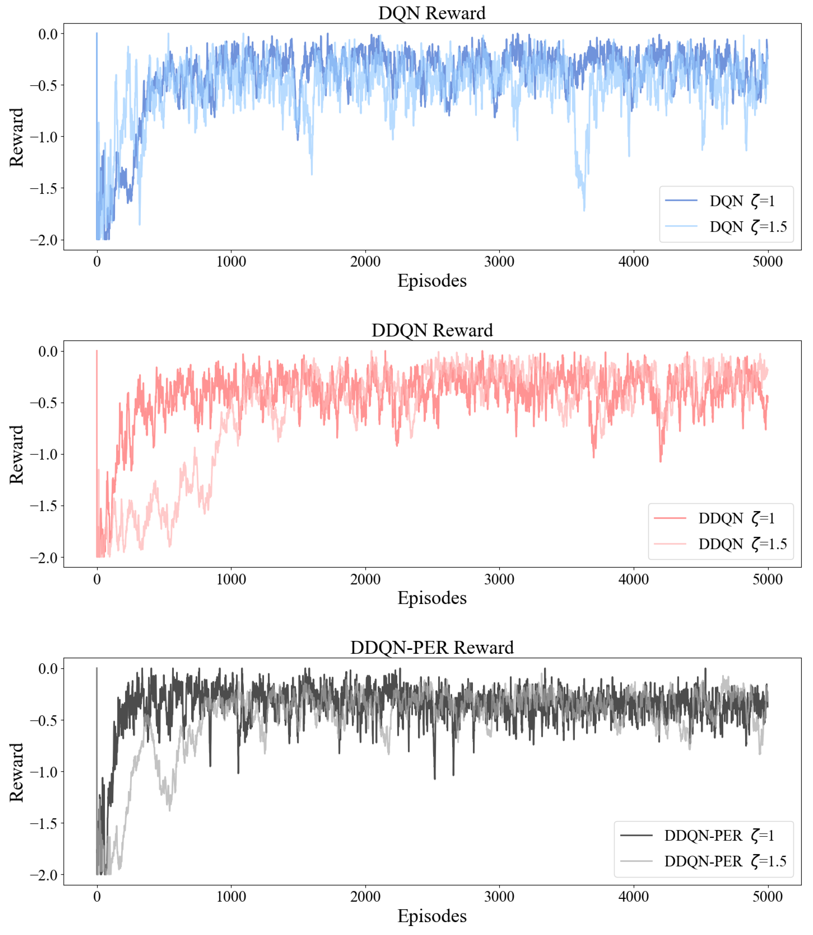
5.3. Convergence Comparison

To enhance algorithm performance in complex scheduling scenarios, this study focuses on several key factors affecting the convergence of reinforcement learning algorithms. Based on the theoretical work by Francisco S. Melo [30], the empirical convergence of the algorithm during training is analyzed from multiple perspectives.

In the in situ data response management environment constructed in this study, the state space is discrete, with each round comprising 3 discrete indicators. The action space is also a discrete and finite set, where the agent can only select one of three queues for response decisions in each round. Therefore, the system satisfies the basic requirements of Q-learning theory regarding a finite state-action space. Meanwhile, the algorithm employs an $ϵ$-greedy strategy for exploration, where $ϵ$ decays from an initial value of 1.0 at a rate of 0.995, effectively ensuring sufficient early exploration and later policy convergence. The learning rate $\alpha$ is fixed at 0.001, which, although not strictly satisfying the Robbins–Monro conditions, has been widely validated for good empirical convergence in small-scale discrete spaces. In addition, the reward function is a negatively weighted combination of indicators with clear upper and lower bounds, ensuring the stability of the value function update process.

In the in situ data management task of the InS system, following a clear algorithm comparison and theoretical convergence analysis, simulation experiments were conducted without limiting the number of training rounds. By observing the variation trends of reward values across training rounds for the three reinforcement learning algorithms, it was found that after a sufficient number of rounds, reward values gradually stabilized with limited fluctuations, and the marginal benefit of increasing the number of training rounds further became negligible.

On this basis, this study sets the maximum number of training rounds to $ma{x}_{e}pochs=5000$, expecting the reinforcement learning algorithms to achieve policy optimization within a limited number of rounds. Meanwhile, to improve the robustness of the experimental results, each algorithm was independently executed $N=10$ times under the premise of fixed training rounds, and the final results were averaged for performance analysis. During training, the adjustment parameter $\zeta$ was varied to further simulate the system’s performance under normal and overloaded conditions. The convergence process of the reward function is shown in Figure 4.

Each subplot illustrates the reward trends of different reinforcement learning algorithms under varying system load levels ($\zeta =1.0$ and $\zeta =1.5$). Since the reward function is dominated by penalty terms, a reward value closer to 0 indicates a better policy selection. Throughout continuous interaction with the environment, all three algorithms exhibit a certain degree of convergence. However, there are noticeable differences in terms of convergence speed and stability. DQN shows considerable fluctuation even in the later training stages, with more pronounced instability under higher load conditions ($\zeta =1.5$). DDQN converges more slowly in the early stages and, despite becoming more stable later, still displays significant reward volatility. By incorporating a prioritized experience replay mechanism, DDQN-PER maintains lower and more stable reward values in the later training phase, demonstrating stronger robustness and convergence performance.

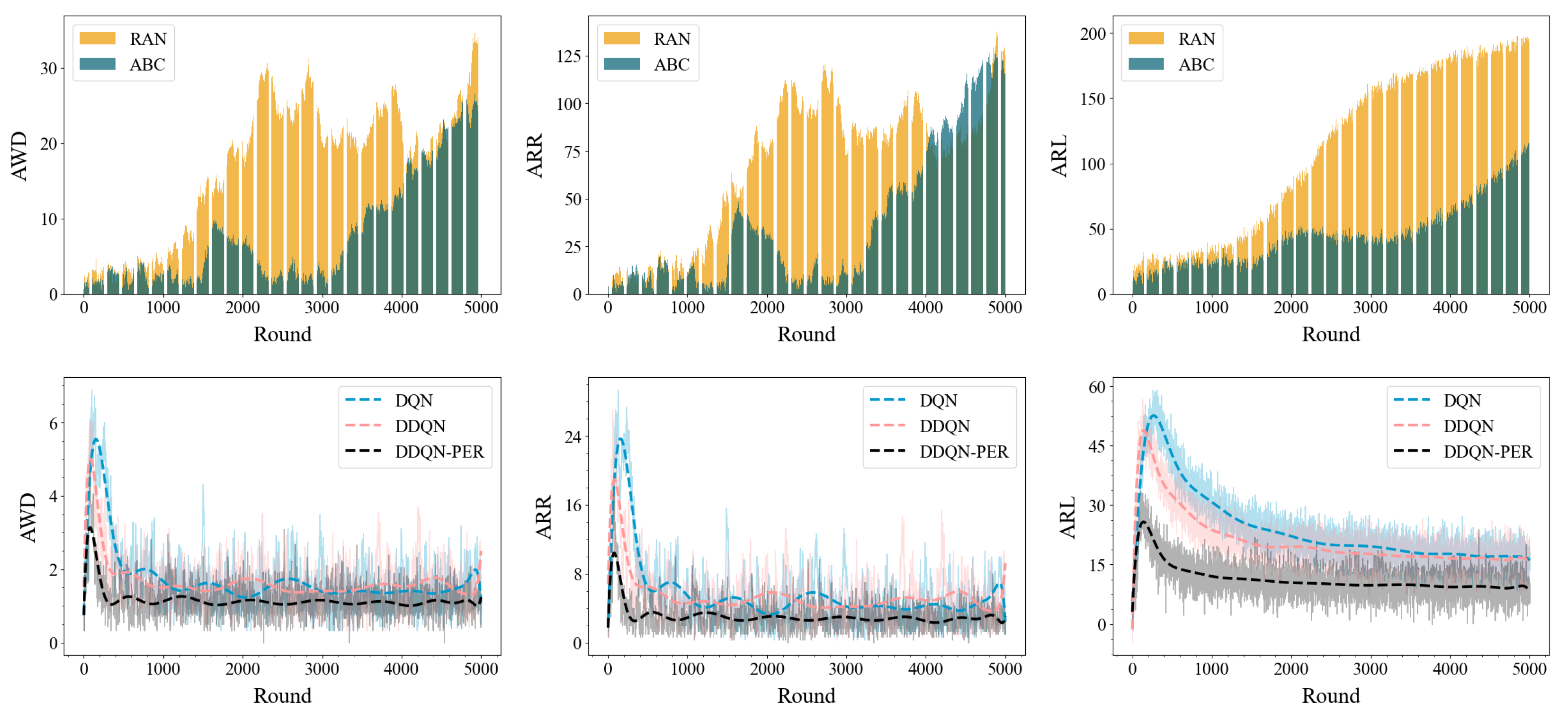
5.4. Comparison of System Metrics

In the in situ data management process of the smart grid InS system, this study uses three system evaluation metrics: AWD, ARR, and ARL, to assess the management strategies driven by different algorithms. To observe the performance of the strategies under different data access demand generation rates, two sets of stress tests are set with $\zeta =1.0$ and $\zeta =2$.

Figure 5 illustrates the performance trends of each algorithm during the experimental process under a system load level of $\zeta =1.0$. Although the static management strategies driven by Baseline and ABC slightly mitigate the growth of system delay and congestion, all three performance metrics continue to rise overall, indicating a lack of effective response and scheduling optimization in complex dynamic environments. In contrast, the three reinforcement learning algorithms are able to learn more optimal scheduling strategies through continuous interaction with the environment. Within the predefined training rounds, all performance indicators exhibit clear convergence trends. Among them, the DDQN-PER algorithm, by introducing a prioritized experience replay mechanism, enhances the learning of critical experiences while improving sampling efficiency, resulting in more efficient policy updates during training. This algorithm outperforms others across all three optimization metrics and demonstrates significant advantages in convergence speed and stability, showcasing stronger generalization capabilities and system adaptability.

Figure 6 illustrates the performance trends of each algorithm during the experiment when the system load increases to $\zeta =1.5$. Compared to the results under $\zeta =1.0$, it is evident that the static management strategies driven by Baseline and ABC almost completely fail under high-load conditions. All three performance indicators continuously rise without exhibiting any convergence trend, indicating a lack of dynamic adaptation and global optimization capability under increased system pressure. In contrast, although the indicator levels of the three reinforcement learning algorithms increase under high load compared to $\zeta =1.0$, they still exhibit convergence trends and remain stable within a relatively small range. These algorithms are capable of continuously optimizing policies and mitigating performance degradation by capturing system state changes. Among them, DDQN-PER demonstrates the most robust adaptability and generalization capability, benefiting from its prioritized experience replay mechanism, which significantly improves sampling efficiency and the utilization of critical experiences. As a result, it surpasses other algorithms in convergence speed, performance stability, and final metric performance.

A comparison of algorithm performance under different system load levels is provided in

Table 4. DDQN + PER algorithm reduction compared to other algorithms for $\zeta =1.0$ and $\zeta =1.5$. This table presents the performance improvements of DDQN-PER compared to other baseline algorithms under different load conditions, with (↓) used to indicate a reduction and optimization in the corresponding indicators.

Comparison	Metric	$\mathit{\zeta }=1.0$	$\mathit{\zeta }=1.5$
DDQN + PER	AWD (↓)	96.83%	99.54%
vs.	ARR (↓)	97.99%	99.76%
Baseline	ARL (↓)	95.28%	99.18%
DDQN + PER	AWD (↓)	95.76%	99.38%
vs.	ARR (↓)	97.87%	99.68%
ABC	ARL (↓)	91.60%	99.09%
DDQN + PER	AWD (↓)	41.93%	5.20%
vs.	ARR (↓)	58.47%	11.73%
DQN	ARL (↓)	45.08%	56.49%
DDQN + PER	AWD (↓)	36.23%	52.99%
vs.	ARR (↓)	53.87%	65.22%
DDQN	ARL (↓)	43.13%	43.94%

.

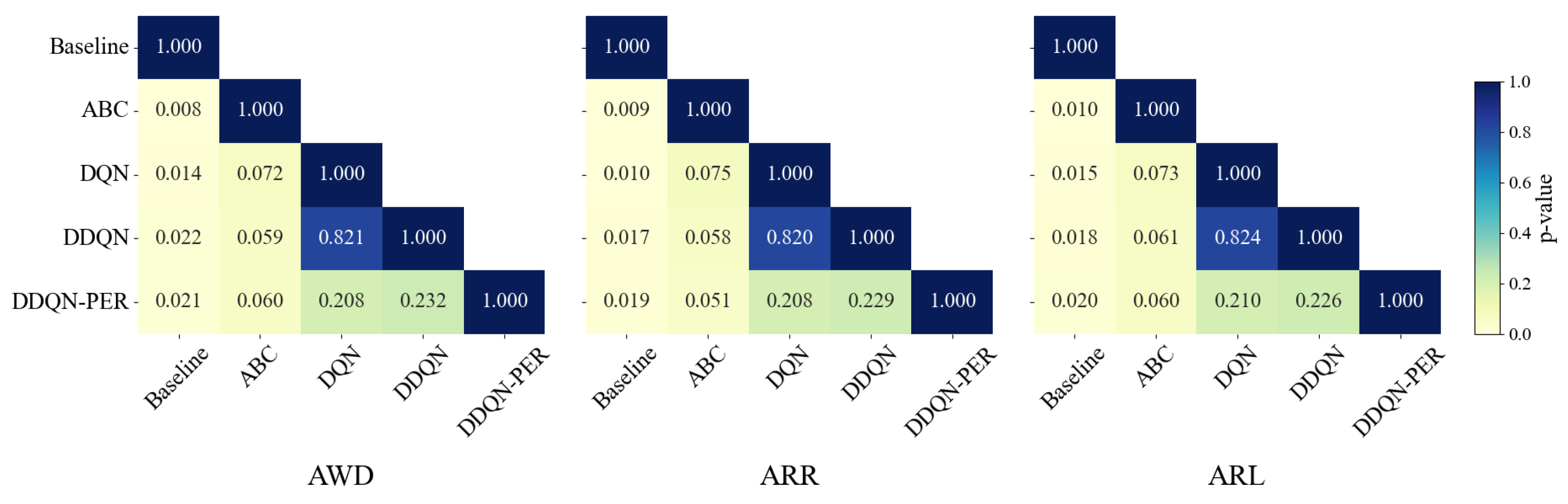
5.5. Statistical Tests

The results were obtained by collecting the average values of evaluation metrics over the final 500 episodes, representing the stable performance of each experiment. Each algorithm yielded 10 sample points for the three system-level evaluation metrics, respectively.

To determine whether the performance differences among algorithms on these metrics are statistically significant, the Friedman test was applied for overall significance analysis. The test results show that the p-values for the three metrics are 0.0008, 0.00015, and 0.0034, respectively, all well below the significance level of 0.05, indicating significant differences among the algorithms on all metrics. Based on this, the Nemenyi post hoc test was further conducted to analyze the pairwise performance differences between algorithms, aiming to reveal which specific algorithm pairs exhibit statistically significant performance disparities. The significance heatmaps of algorithmic differences under the three metrics are illustrated in Figure 7.

While the above tests focus on performance differences between algorithms, this study also evaluates within-group consistency by introducing the Fleiss’ Kappa coefficient to measure the stability and behavioral consistency of similar algorithms under repeated experimental runs. The five algorithms were divided into two groups for consistency analysis: the traditional group (Baseline and ABC) and the reinforcement learning group (DQN, DDQN, and DDQN-PER). Based on the existing average values, normalization and discretization were performed to obtain $AW{D}^{\mathrm{disc}}$, $AR{R}^{\mathrm{disc}}$, and $AR{L}^{\mathrm{disc}}$.

Referring to the interpretation standards of the Kappa coefficient proposed by Landis and Koch [31], we evaluated the consistency of each algorithm across the three metrics, and the final results are shown in

Table 5. Fleiss’ Kappa analysis results (algorithm consistency). This table presents the Fleiss’ Kappa coefficients and corresponding consistency interpretations for different algorithm groups across three metrics, reflecting the level of agreement among algorithms.

Algorithm Group	Metric	Fleiss’ Kappa	Consistency Interpretation
Baseline, ABC	AWD	0.12	Slight consistency
	ARR	0.08	Poor consistency
	ARL	0.15	Slight consistency
DQN, DDQN, DDQN-PER	AWD	0.45	Moderate consistency
	ARR	0.52	Moderate consistency
	ARL	0.36	Fair consistency

. The consistency of traditional algorithms across all three metrics is relatively low, with kappa values all below 0.2, indicating that non-learning-based algorithms exhibit considerable fluctuations in dynamic environments and inconsistent behavioral patterns. In contrast, the reinforcement learning group demonstrates significantly higher consistency, suggesting that reinforcement learning strategies develop stable and convergent decision behaviors through repeated training.

6. Conclusions

This paper focuses on the in situ (InS) system in the context of smart grid environments and proposes a comprehensive optimization management scheme for in situ data generated by sensors, effectively improving data processing efficiency and system response capability. To address the issues in traditional storage schemes, such as low storage efficiency and slow access speed caused by the lack of data demand classification, this paper abstracts servers with different performance levels into a hierarchical storage structure and designs an in situ data classification mechanism to allocate data to different server layers based on their characteristics, thereby optimizing storage and access paths from the source. Furthermore, a personalized demand queue architecture is introduced to enable the classified reception of diverse requests, enhancing the system’s task-handling capability under high-concurrency scenarios. To achieve intelligent scheduling and response, a demand response strategy driven by the DDQN-PER algorithm is adopted, which ensures system stability while optimizing overall latency and queue congestion. The proposed method reduces average waiting delay and response delay by 67.69% and 68.7%, respectively, compared to traditional algorithms and other reinforcement learning methods, while the number of residual unserved demands is reduced by an average of 77.05%. The overall scheme maintains strong timeliness and responsiveness under various load conditions, and also demonstrates good scalability and robustness, effectively supporting the growing data management demands in in situ systems, thus exhibiting strong practical value and theoretical contribution.

References

1. Krishna, M.S.R.; Khasim Vali, D. Meta-RHDC: Meta Reinforcement Learning Driven Hybrid Lyrebird Falcon Optimization for Dynamic Load Balancing in Cloud Computing. IEEE Access 2025, 13, 36550–36574. [Google Scholar] [CrossRef]
2. Cheng, Z.; Zhang, L.; Hao, Z.; Qu, S.; Liu, J.; Ding, X.; Liu, C.; Li, N.; Li, R. Assisting Offshore Production Optimization Technology in Intelligent Completion Operation Based on Edge-Cloud Collaborative Technologies. In Proceedings of the Abu Dhabi International Petroleum Exhibition and Conference, Abu Dhabi, United Arab Emirates, 4–7 November 2024; SPE: Houston, TX, USA, 2024; p. D021S037R003. [Google Scholar]
3. Li, J.; Xia, Y.; Sun, X.; Chen, P.; Li, X.; Feng, J. Delay-Aware Service Caching in Edge Cloud: An Adversarial Semi-Bandits Learning-Based Approach. In Proceedings of the 2024 IEEE 17th International Conference on Cloud Computing (CLOUD), Shenzhen, China, 7–13 July 2024; IEEE: Piscataway, NJ, USA, 2024; pp. 411–418. [Google Scholar]
4. Zhang, L.; Hao, P.; Zhou, W.; Ma, J.; Li, K.; Yang, D.; Wan, J. A thermostatically controlled loads regulation method based on hybrid communication and cloud–edge–end collaboration. Energy Rep. 2025, 13, 680–695. [Google Scholar] [CrossRef]
5. Wu, D.; Li, Z.; Shi, H.; Luo, P.; Ma, Y.; Liu, K. Multi-Dimensional Optimization for Collaborative Task Scheduling in Cloud-Edge-End System. Simul. Model. Pract. Theory 2025, 141, 103099. [Google Scholar] [CrossRef]
6. Xiao, L.; Jia, G.; Lin, X. Construction of Manufacturing Data Acquisition System Based on Edge Computing. In Proceedings of the 2024 International Conference on Computers, Information Processing and Advanced Education (CIPAE), Ottawa, ON, Canada, 26–28 August 2024; IEEE: Piscataway, NJ, USA, 2024; pp. 571–576. [Google Scholar]
7. Wan, Z.; Zhao, S.; Dong, X.; Huang, Z.; Tan, Y. Joint DRL and ASL-Based “Cloud-Edge-End” Collaborative Caching Optimization for Metaverse Scenarios. In Proceedings of the 2024 IEEE 30th International Conference on Parallel and Distributed Systems (ICPADS), Belgrade, Serbia, 10–14 October 2024; IEEE: Piscataway, NJ, USA, 2024; pp. 342–349. [Google Scholar]
8. Hasan, N.; Alam, M. Role of machine learning approach for industrial internet of things (IIoT) in cloud environment-a systematic review. Int. J. Adv. Technol. Eng. Explor. 2023, 10, 1391. [Google Scholar]
9. Tang, Y. Tiansuan Constellation: Intelligent Software-Defined Microsatellite with Orbital Attention for Sustainable Development Goals. In Proceedings of the International Conference on Big Data Intelligence and Computing, Shanghai, China, 16–18 December 2022; Springer: Berlin/Heidelberg, Germany, 2022; pp. 3–21. [Google Scholar]
10. Zeng, L.; Ye, S.; Chen, X.; Zhang, X.; Ren, J.; Tang, J.; Yang, Y.; Shen, X.S. Edge Graph Intelligence: Reciprocally Empowering Edge Networks with Graph Intelligence. IEEE Commun. Surv. Tutorials 2025, 27, 1–16. [Google Scholar] [CrossRef]
11. Leng, J.; Chen, Z.; Sha, W.; Ye, S.; Liu, Q.; Chen, X. Cloud-edge orchestration-based bi-level autonomous process control for mass individualization of rapid printed circuit boards prototyping services. J. Manuf. Syst. 2022, 63, 143–161. [Google Scholar] [CrossRef]
12. Xiao, J.; Wang, Y.; Zhang, X.; Luo, G.; Xu, C. Multi source data security protection of smart grid based on edge computing. Meas. Sens. 2024, 35, 101288. [Google Scholar] [CrossRef]
13. Hong, H.; Suo, Z.; Wu, H.; Li, D.; Wang, J.; Lu, H.; Zhang, Y.; Lu, H. Large-scale heterogeneous terminal management technology for power Internet of Things platform. In Proceedings of the 2022 2nd International Conference on Consumer Electronics and Computer Engineering (ICCECE), Guangzhou, China, 14–16 January 2022; IEEE: Piscataway, NJ, USA, 2022; pp. 161–164. [Google Scholar]
14. He, X.; Dong, H.; Yang, W.; Li, W. Multi-source information fusion technology and its application in smart distribution power system. Sustainability 2023, 15, 6170. [Google Scholar] [CrossRef]
15. Zeng, F.; Pang, C.; Tang, H. Sensors on internet of things systems for the sustainable development of smart cities: A systematic literature review. Sensors 2024, 24, 2074. [Google Scholar] [CrossRef]
16. Li, C.; Hu, Y.; Liu, L.; Gu, J.; Song, M.; Liang, X.; Yuan, J.; Li, T. Towards sustainable in-situ server systems in the big data era. ACM Sigarch Comput. Archit. News 2015, 43, 14–26. [Google Scholar] [CrossRef]
17. Cisco. Cisco Technology Radar Trends, 2014. White Paper. Available online: https://davidhoglund.typepad.com/files/tech-radar-trends-infographics.pdf (accessed on 15 May 2025).
18. Zhang, F.; Lasluisa, S.; Jin, T.; Rodero, I.; Bui, H.; Parashar, M. In situ feature-based objects tracking for large-scale scientific simulations. In Proceedings of the 2012 SC Companion: High Performance Computing, Networking Storage and Analysis, Salt Lake City, UT, USA, 10–16 November 2012; IEEE: Piscataway, NJ, USA, 2012; pp. 736–740. [Google Scholar]
19. Lakshminarasimhan, S.; Boyuka, D.A.; Pendse, S.V.; Zou, X.; Jenkins, J.; Vishwanath, V.; Papka, M.E.; Samatova, N.F. Scalable in situ scientific data encoding for analytical query processing. In Proceedings of the 22nd International Symposium on High-Performance Parallel and Distributed Computing, New York, NY, USA, 17–21 June 2013; pp. 1–12. [Google Scholar]
20. Park, J.; Choi, S.; Kim, J.; Koo, G.; Yoon, M.K.; Oh, Y. TM-Training: An Energy-Efficient Tiered Memory System for Deep Learning Training in NPUs. ACM Trans. Storage, 2025; in press. [Google Scholar] [CrossRef]
21. Anjum, M.; Kraiem, N.; Min, H.; Dutta, A.K.; Daradkeh, Y.I.; Shahab, S. Opportunistic access control scheme for enhancing IoT-enabled healthcare security using blockchain and machine learning. Sci. Rep. 2025, 15, 7589. [Google Scholar] [CrossRef] [PubMed]
22. Guan, H.; Yu, L.; Zhou, L.; Xiong, L.; Chowdhury, K.; Xie, L.; Xiao, X.; Zou, J. Privacy and Accuracy-Aware AI/ML Model Deduplication. arXiv 2025, arXiv:2503.02862. [Google Scholar]
23. Yuan, Q.; Pi, Y.; Kou, L.; Zhang, F.; Li, Y.; Zhang, Z. Multi-source data processing and fusion method for power distribution internet of things based on edge intelligence. Front. Energy Res. 2022, 10, 891867. [Google Scholar] [CrossRef]
24. Zielosko, B.; Jabloński, K.; Dmytrenko, A. Exploiting Data Distribution: A Multi-Ranking Approach. Entropy 2025, 27, 278. [Google Scholar] [CrossRef] [PubMed]
25. Liu, F.; Tang, G.; Li, Y.; Cai, Z.; Zhang, X.; Zhou, T. A survey on edge computing systems and tools. Proc. IEEE 2019, 107, 1537–1562. [Google Scholar] [CrossRef]
26. Nain, G.; Pattanaik, K.; Sharma, G. Towards edge computing in intelligent manufacturing: Past, present and future. J. Manuf. Syst. 2022, 62, 588–611. [Google Scholar] [CrossRef]
27. Van Hasselt, H.; Guez, A.; Silver, D. Deep reinforcement learning with double q-learning. In Proceedings of the AAAI Conference on Artificial Intelligence, Phoenix, AZ, USA, 12–17 February 2016; Volume 30. [Google Scholar]
28. Schaul, T.; Quan, J.; Antonoglou, I.; Silver, D. Prioritized experience replay. arXiv 2015, arXiv:1511.05952. [Google Scholar]
29. Xiong, X.; Zheng, K.; Lei, L.; Hou, L. Resource Allocation Based on Deep Reinforcement Learning in IoT Edge Computing. IEEE J. Sel. Areas Commun. 2020, 38, 1133–1146. [Google Scholar] [CrossRef]
30. Melo, F.S. Convergence of Q-Learning: A Simple Proof; Technical Report; Institute of Systems and Robotics, University of Coimbra: Coimbra, Portugal, 2001; pp. 1–4. [Google Scholar]
31. Landis, J.R.; Koch, G.G. The measurement of observer agreement for categorical data. Biometrics 1977, 33, 159–174. [Google Scholar] [CrossRef] [PubMed]
Figure 2. System Modeling Process. This figure provides a detailed illustration of the system modeling process, including in situ data generation, classification, storage, and access demand generation.
Applsci 15 05980 g002
Figure 3. DDQN-PER Algorithm Structure. This figure illustrates in detail the workflow of the DDQN-ER algorithm, clearly depicting the complete process from environment state perception, action selection by the policy and target networks, to the experience replay mechanism and network parameter updates. It comprehensively reflects the execution logic and core mechanisms of the algorithm in decision-making optimization.
Applsci 15 05980 g003
Figure 4. Convergence performance. This figure illustrates the reward convergence process of three reinforcement learning comparison algorithms within a limited number of episodes. It also compares the reward convergence trends of each algorithm under different system load conditions ( ζ = 1.0 and ζ = 1.5 ).
Applsci 15 05980 g004
Figure 5. The system performance comparison when ζ = 1.0 . The trends of all three performance indicators under different algorithms within a limited number of training episodes are illustrated. The first row presents the indicator variations for the two traditional algorithms, while the second row shows the results for the three reinforcement learning algorithms. The colored shaded areas represent the fluctuation range across ten independent experiments. Polynomial fitting is applied to these areas to highlight the overall trend of the indicators.
Applsci 15 05980 g005
Figure 6. The system performance comparison when ζ = 1.5 . The trends of all three performance indicators under different algorithms within a limited number of training episodes are illustrated. The first row presents the indicator variations for the two traditional algorithms, while the second row shows the results for the three reinforcement learning algorithms. The colored shaded areas represent the fluctuation range across ten independent experiments. Polynomial fitting is applied to these areas to highlight the overall trend of the indicators.
Applsci 15 05980 g006
Figure 7. Pairwise Nemenyi post hoc p-value heatmaps across three evaluation metrics. This figure presents the p-value heatmaps of the Nemenyi post hoc pairwise comparison tests conducted after the Friedman test, corresponding to the three different performance evaluation metrics. Each heatmap illustrates whether the performance differences between any two algorithms under the given metric are statistically significant. Lower p-values indicate more significant differences. Typically, p-values below 0.05 are considered significant. The matrices are symmetric, with only the lower triangular region displayed to improve readability. All three heatmaps share a common color scale to unify the visualization of p-values.
Applsci 15 05980 g007