Low-Cost Solution for Kinematic Mapping Using Spherical Camera and GNSS

Abstract

The use of spherical cameras for mapping purposes is a common application in surveying. Very expensive and high-quality cameras are used for surveying purposes and are supplemented by systems for determining their position. Cheap cameras, in most cases, only complement laser scanners, and the images are then used to color the laser point cloud. This article investigates the use of action cameras in combination with low-cost GNSS (Global Navigation Satellite System) equipment. The research involves the development of a methodology and software for georeferencing spherical images, created by the kinematic method, using GNSS RTK (Real-Time Kinematics) or PPK (Post-Processing Kinematics) coordinates. Testing was carried out in two case studies where the environment surveyed had varying properties. Considering that the images from the low-cost 360 camera are of lower quality, an artificial intelligence tool was used to improve the quality of the images. The point clouds from a low-cost device are compared with more accurate methods. One of them is the SLAM (Simultaneous Localization and Mapping) method with the Faro Orbis device. The results in this work show sufficient accuracy and data quality for mapping purposes. Due to the very low price of the low-cost device used in this work, it is very easy to extend this method to practice.

1. Introduction

Spherical cameras with a 360° view have recently become very popular for taking personal sports videos, panoramic photos, and creating virtual tours of an object. Due to this trend, these cameras have also become more affordable, more powerful, lighter, and more compact. All these aspects are also important for the use of spherical cameras in surveying and mapping tasks.

The first spherical cameras for mapping appeared in the first half of the twentieth century. To create a panoramic image, wide-angle lenses or multi-lens systems were often used that transferred the scene to one central lens [1]. After the arrival of digital cameras at the turn of the millennium, the first modern mobile mapping systems (MMSs) were developed. However, this required the development and release of technical subsystems for civilian use. First came the original GPS (Global Positioning System), the GNSSS came later, and then the IMUs (Inertial Measurement Units) came. GNSS senses spatial coordinates, while IMU senses acceleration using accelerometers and rotational angles using gyroscopes. Subsequent INSs (Inertial Navigation Systems) contained more accurate IMUs and were supplemented with additional algorithms such as Kalman filters for precise positioning. MMSs use multiple cameras for panoramic imaging, laser scanning heads, and GNSS/IMU or GNSS/INS systems for georeferencing data [2,3]. With the rise of Google Street View, panoramic photography, known as Street View, became very popular. To create these spherical images, cameras created by several sensors with low-distortion lenses were used [4]. This principle of using multiple sensors is used in most measurement cameras such as the Ladybug5 [5,6] or even in cameras that are part of a multisensory mapping device [7]. Subsequently, in the second decade of the 20th century, personal mapping laser systems (PLSs) appeared, carried by operators or in the form of backpacks, such as, most famously, the Leica Pegasus [8]. Smaller PLSs are mainly used in enclosed spaces where there is no GNSS signal. In this case, SLAM technology is used to determine the position of the device and its trajectory. In most cases, this technology uses a laser scanner to map the surroundings while the operator is moving [9,10].

Spherical action cameras have a very similar design; spherical photos are created using two sensors with wide-angle lenses [11]. These cameras have already been tested for indoor modeling purposes, but also for exterior measurement [12,13,14]. The articles report a standard deviation of static imaging up to 8 cm. However, in good lighting conditions, in a nonhomogeneous environment, the resulting spatial accuracy of tens of mm can be achieved. The precision in the kinematic measurement of indoor objects varies between 2 and 10 cm, depending on the type of camera and the quality of its output [15,16].

Compared to professional cameras, these low-cost action cameras, due to their design, have more problems with the blurring of images, lower image quality, and a non-standard model of distortion of the panoramic image, and when shooting in poorly lighted places. The problem of low-resolution images can be reduced by using artificial intelligence tools [17] and a deep convolutional neural network (DCNN) [18]. The Enhanced Super-Resolution Generative Adversarial Network (ESRGAN) [19,20] architecture, which aims to predict high-resolution images from corresponding low-resolution images, finds applications in photogrammetry.

The Structure-from-Motion method [21], in combination with the Multi-View Stereo (SfM-MVS), is suitable for the reconstruction of 3D environments from spherical images. This method is low-cost and easy to use; the positions and orientations of the cameras are determined automatically by iterative computation. However, to use this method, it is necessary to have many overlapping images that contain clearly identifiable points, and it is important that the images are taken close to each other. As the name suggests, the carrier must be in motion when collecting image data, and the images taken must capture the object of interest from different positions [22,23,24,25].

Many projects also deal with mapping and visualizing interior spaces using panoramic cameras in virtual museum projects [26,27,28].

When measuring outdoors, it is useful to equip the low-cost camera with a GNSS. As with professional mapping devices, georeferenced imagery will provide easier photo alignment, and fewer ground control points will be needed in the field. The resulting cloud accuracy depends on the type of method used. When data are collected using static photos and GNSS RTK measurements, a final point cloud accuracy of around 3 cm can be achieved. The problem comes with the kinematic method: data collection is achieved through video recording, where even in a relatively suitable environment for GNSS measurements, 2D clouds reach an accuracy of 17–20 cm. This problem is most likely due to the asynchronization of camera time and GNSS time [29].

This article focuses on mapping using the low-cost Insta360 X3 camera in conjunction with low-cost GNSS equipment [30]. For this work, software and methodologies were developed that enable georeferencing of the taken spherical images with GNSS RTK or GNSS PPK coordinates. Special attention is given to testing a novel method of image georeferencing based on a visual timestamp synchronization of the spherical camera. Furthermore, the study investigates the potential of artificial intelligence tools to improve the quality of mapping outputs, particularly in point cloud generation and orthophoto production. The article also includes tests of this method against GNSS RTK ground points and mobile scanning with the Faro Orbis device using the SLAM method.

2. Materials and Methods

This chapter focuses on the description of test sites, the definition of GCPs (ground control points), checkpoints, the description of low-cost mapping equipment, and the processing of the collected data.

2.1. Materials

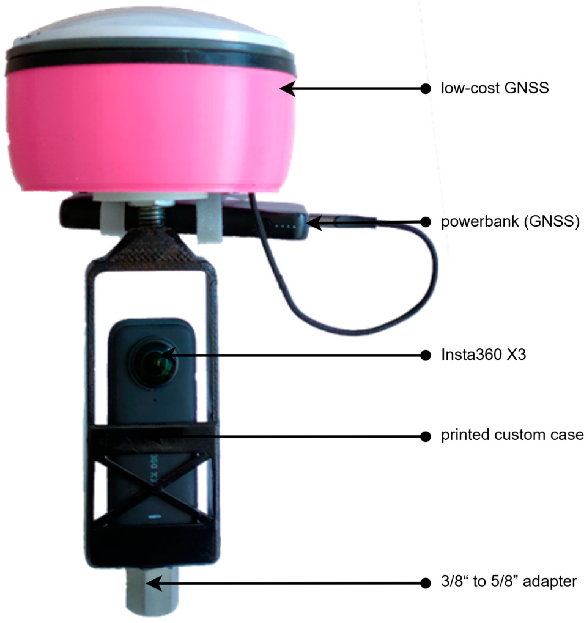
The main part of the low-cost device is the Insta360 X3 spherical camera (Arashi Vision Inc., Shenzhen, China). This camera is equipped with a 1/2″ sensor to capture 360° videos at resolutions up to 5.7K/30fps. The camera includes two fisheye lenses with a focal length of 6.7 mm and an aperture of F1.9. The camera also includes an inertial system that allows it to stabilize the orientation of the images. All data collected are stored in an INSV format.

Another important part of the equipment is the low-cost GNSS. The GNSS consists of a ZED-F9P receiver and an Ardusimple ANT2B antenna [24] (ArduSimple, Lleida, Spain). The GNSS Controller application, developed by students at CTU Prague, is used to record RTK positions and log RAW data. The accuracy of RTK σ measurements is 1 cm + 1 ppm, as specified by the receiver manufacturer.

To integrate these components into a single device, a custom case was designed to securely hold both devices. This assembled device can then be mounted on a pole. The important thing is not to obscure the GNSS antenna with devices that could interfere with the reception of the GNSS signal. The complete low-cost device is shown in Figure 1.

A Trimble R2 GNSS device (Trimble Inc., Westminster, CO, USA) was used to create a reference absolute point field based on GCPs. In the Lipová street case study, several checkpoints were surveyed using a Trimble S8 total station. The reference point clouds were created using a Faro Orbis mobile scanning system, where the manufacturer specifies a one-sigma 5 mm accuracy, and a Mavic 3E drone (SZ DJI Technology Co., Ltd., Shenzhen, China) with an RTK module.

2.2. Ground Control Points and Checkpoints

For the purposes of georeferencing and accuracy evaluation, several ground control points (GCPs) and checkpoints were established at each test site. The GCPs were physically stabilized using a surveying spike with a hole for the precise placement of a pole tip. Each point was marked by a high-contrast 10 × 10 cm checkerboard target, a rigid plate, or fluorescent spray, depending on surface conditions.

In addition to artificially marked points, several checkpoints were selected from spatially well-defined features such as corners of fences, buildings, or sidewalks, where precise identification in the images was possible.

All GNSS measurements, both from the low-cost GNSS system and the reference Trimble R2 receiver (Trimble Geospatial, Dubai, United Arab Emirates), were recorded in the ETRS89 coordinate system (realization of ETRF2000), as defined by the CZEPOS network.

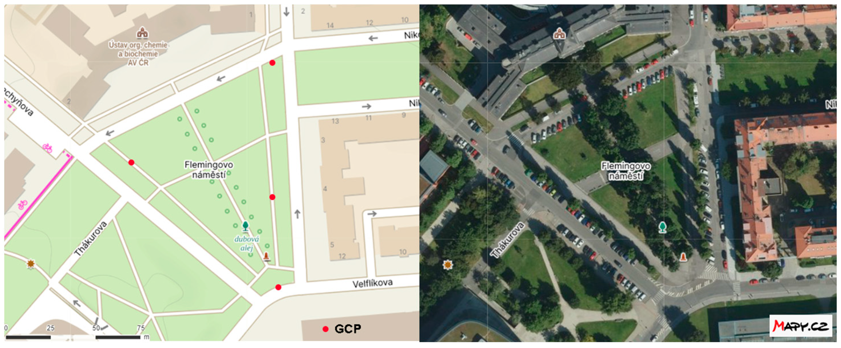
2.3. Case Study—Fleming Square, Prague

The Fleming Square (50.1050564 N, 14.3918744 E) test site (Figure 2) was chosen for two reasons. This area is close to the CTU campus in Prague, and there are fully grown trees in the square. Due to these reasons, there is jamming of the GNSS signal, and the measurements are more relevant to the real measurement conditions.

At this site, the necessary GCPs were measured using the GNSS RTK method. Together four GCPs were measured and used in the following processing. The GCPs were measured three times, and the 3D standard deviation was calculated from their differences. The 3D standard deviation of the GCPs was 20 mm, and deviations of the GNSS RTK measurements are shown in

Table 1. Standard deviations of the GNSS RTK point field: Fleming Square.

St. Dev. XY [mm]	St. Dev. Z [mm]	St. Dev. XYZ [mm]
11	17	20

. The square was also surveyed using the Faro Orbis mobile scanning method and the SLAM method.

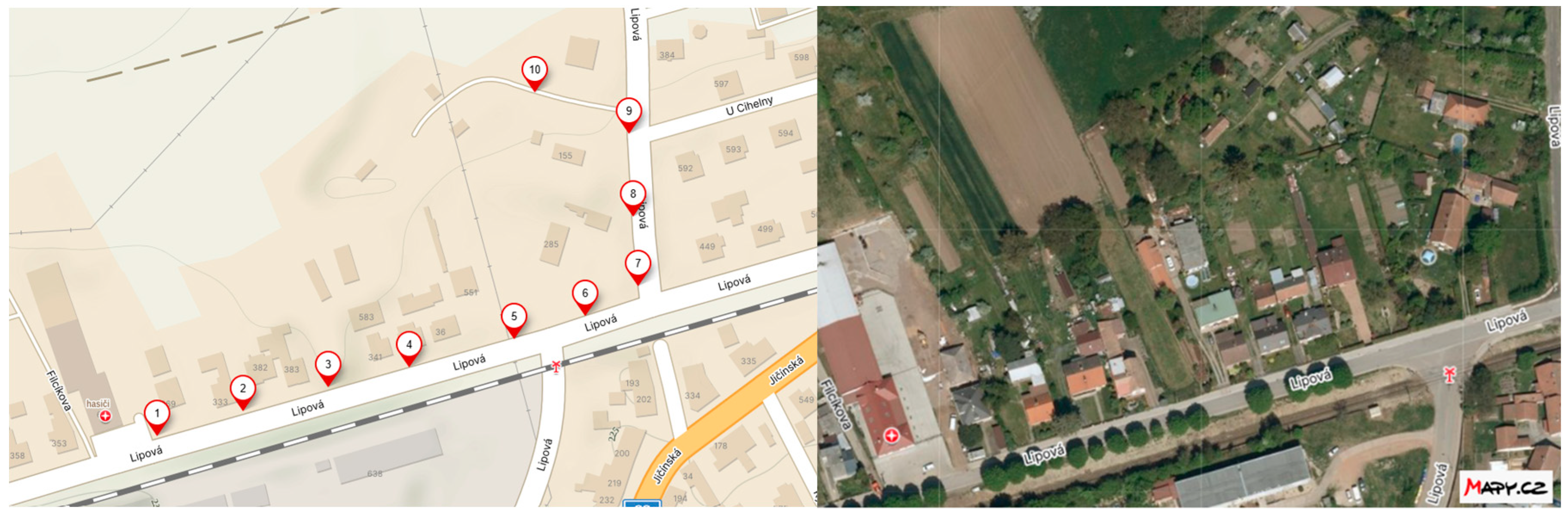
2.4. Case Study—Lipová Street, Kopidlno

The measured street is in the small town of Kopidlno (50.3362019 N, 15.2695339 E) in the north of the Czech Republic (Figure 3). In this place, a detailed survey was recently carried out by the Cadastral Office for the purposes of the cadastral, which uses only XY coordinates. The cadastral points in this area were used as a basis for referencing because several checkpoints (e.g., fence and building corners) were surveyed using a Trimble S8 total station (Precision Laser & Instrument, Inc., Columbus, OH, USA) with reflectorless EDM, directly referencing these cadastral markers. Since the official cadastral coordinates are defined in the national S-JTSK coordinate system, they were transformed into ETRS89. The GNSS RTK method was used to independently verify the coordinates of 10 selected points. The standard deviations of the differences between the cadastral coordinates and the GNSS-measured coordinates are given in

Table 2. Standard deviation of the differences between the cadastral coordinates and the GNSS RTK-measured coordinates.

St. Dev. XY [mm]
23 mm

. Only the first 7 points were used for referencing and checking, as the others had a higher error due to the tall trees along the street.

The area was also mapped by photogrammetry using a Mavic 3E drone (DJI Enterprise, New York, NY, USA) with an RTK module. The point cloud was calculated in the Agisoft Metashape software ver. 2.0.1 [31]. It was aligned using 3D coordinates derived from 7 cadastral points that were verified and supplemented with height information from GNSS RTK measurements. Among these, 3 points were used as GCPs for referencing, while the remaining 4 were used as independent checkpoints. The standard deviations of the differences in the checkpoints can be found in

Table 3. Standard deviations of the differences between the GNSS RTK points and the points given from the Mavic 3E point cloud.

St. Dev. XY [mm]	St. Dev. Z [mm]	St. Dev. XYZ [mm]
49 mm	28 mm	56 mm

.

2.5. Measurement Methods

The measurement process itself is very simple with low-cost equipment. The assembled device, made of an Insta360 X3 camera and a low-cost GNSS, was placed on a geodetic pole at a height of about 2 m so that the surveyor covers a small part of the camera’s field of view. The low-cost GNSS device was paired with the phone via Bluetooth and the GNSS Controller mobile app, and after a short initialization, the GNSS RTK and RAW data collection started. For post-processing time synchronization between the images and the GNSS, the mobile device screen was recorded for a few seconds before each data collection session began in order to record a graphical clock with a very precise time (Figure 4).

The area of interest was then measured by the walk method with the device at a speed of 4–5 km/h in a closed loop. During the measurements, an effort was made to avoid places with an obscured view of the sky to prevent degradation of the GNSS signal, but this was not always possible. To ensure sufficient accuracy in locations with poorer GNSS signals and corner areas, the carrier speed was partially reduced.

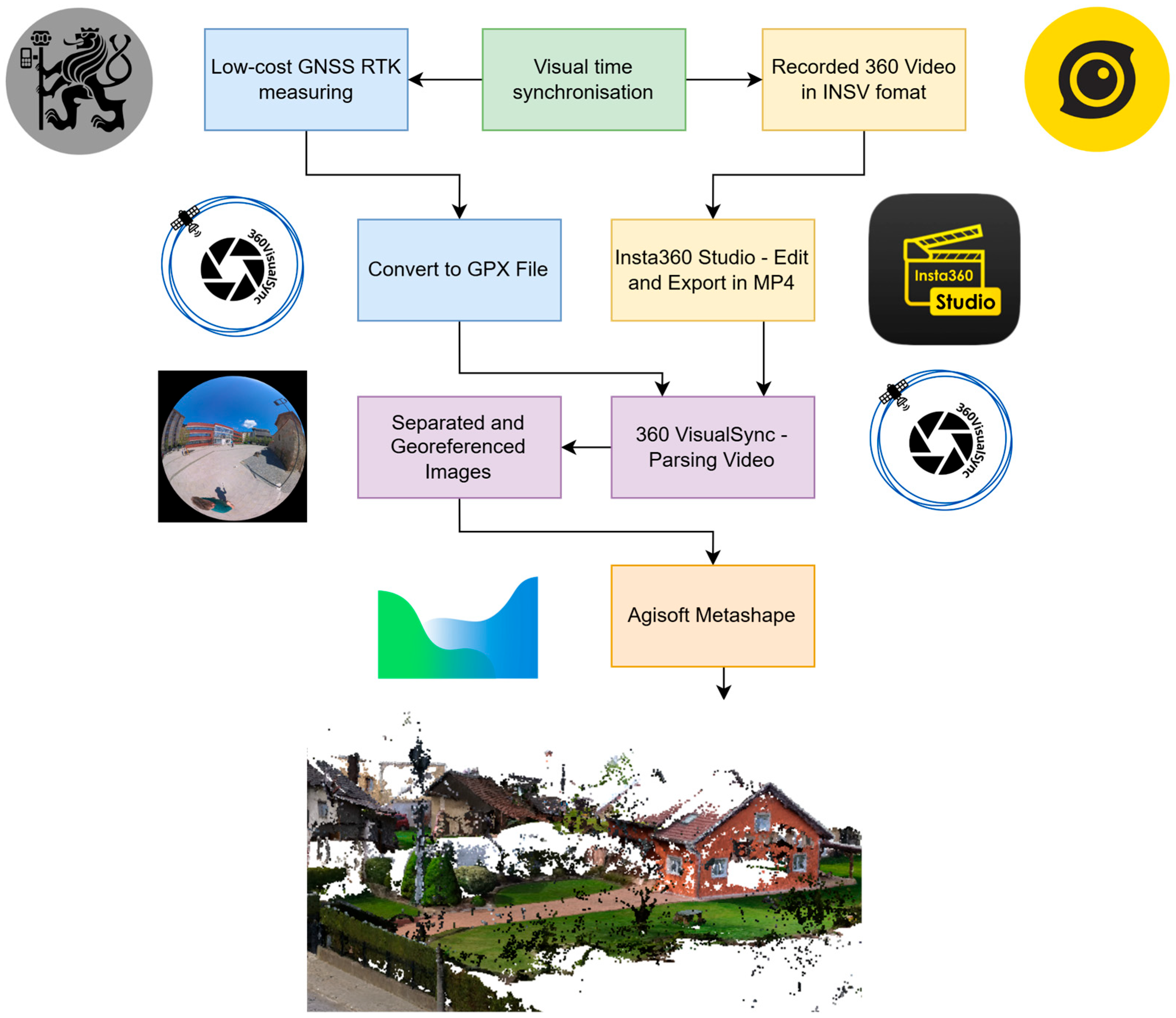
2.6. Processing Methods

The collected data had to be first converted to video; then, the individual images were separated, the position was assigned, and a 3D reconstruction of the focused area was performed. Several software tools were used to process the measured data, including one developed for this project, 360VisualSync (https://github.com/Luckays/360VisualSync, accessed on 7 March 2025). Figure 5 shows a graph of low-cost mobile mapping processing.

2.6.1. Insta360 Studio

In this software [32], the video from the two sensors was stitched together into a single video. The data were kept without significant editing and image stabilization. The spherical video was exported in an MP4 format, an encoding format of H.264, and a bitrate of 120 Mbps. The export time of a 10 min video is around 25 min.

2.6.2. 360VisualSync

The software offers several ways to process video: video parsing, time stamping, and geotagging. The software is available at https://github.com/Luckays/360VisualSync, accessed on 7 March 2025.

The basic function is just to parse the video into single frames at 1 s intervals. After entering the beginning time of the video captured from the visual synchronization of the first frame, the software assigns UTC time to the single frames. If a GPX file with measured coordinates is provided to the software, these coordinates and their accuracies are written to the individual images. In case of missing coordinates, the software calculates the approximate position of the images for easier alignment in the following software. Using this software, it is possible to carry out geotagging with RTK or PPK GNSS coordinates.

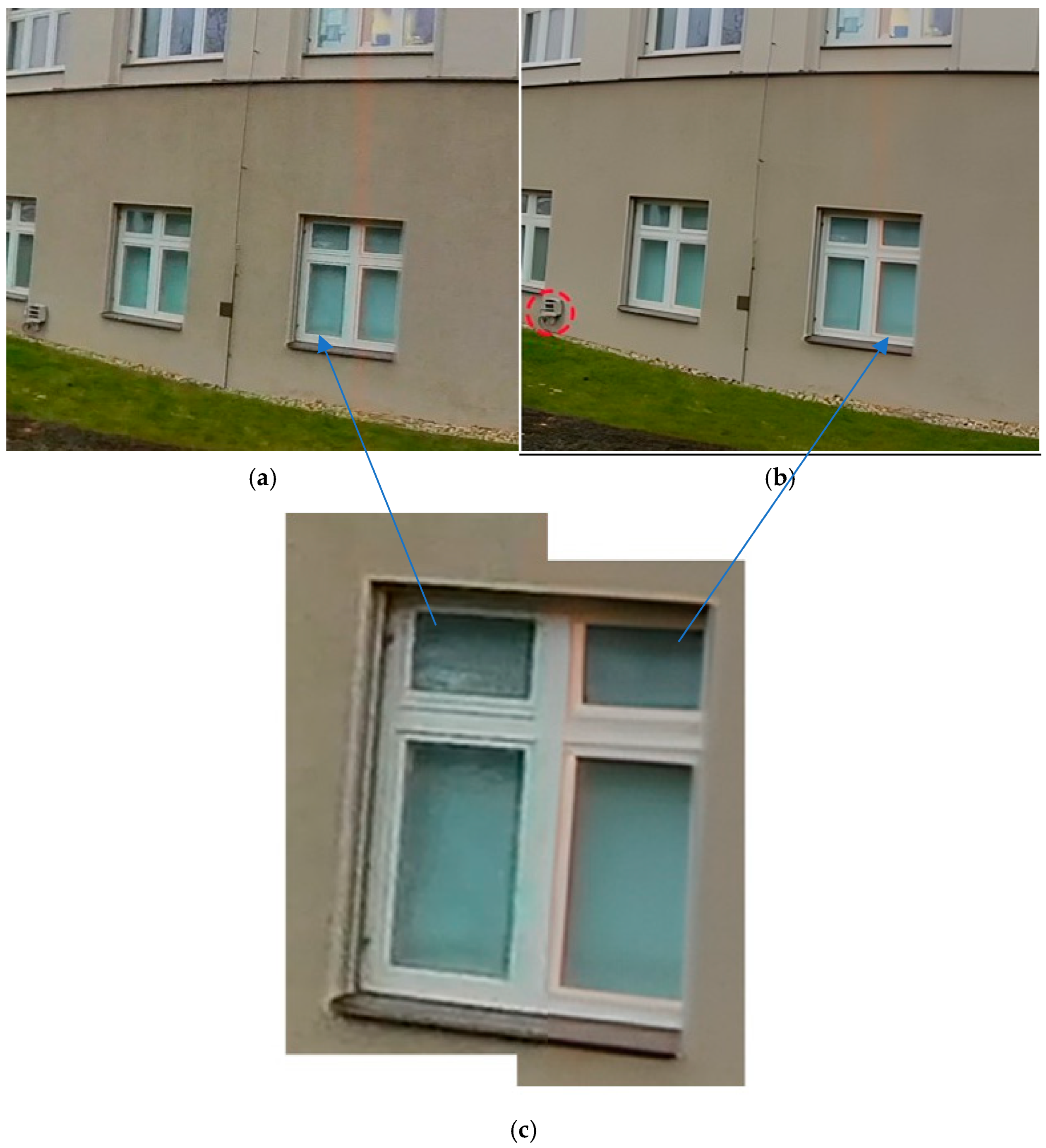
2.6.3. Real-ESRGAN

Since the images captured from the spherical camera video are of lower quality compared to taking single images, one set of images was edited by artificial intelligence tools. For this purpose, Real-ESRGAN [33] software (https://github.com/xinntao/Real-ESRGAN, accessed on 20 March 2024) was used, which aims to improve image quality and resolution by using machine learning. For this project, the already pre-trained realesrnet-x4plus model was included in the 360VisualSync app. 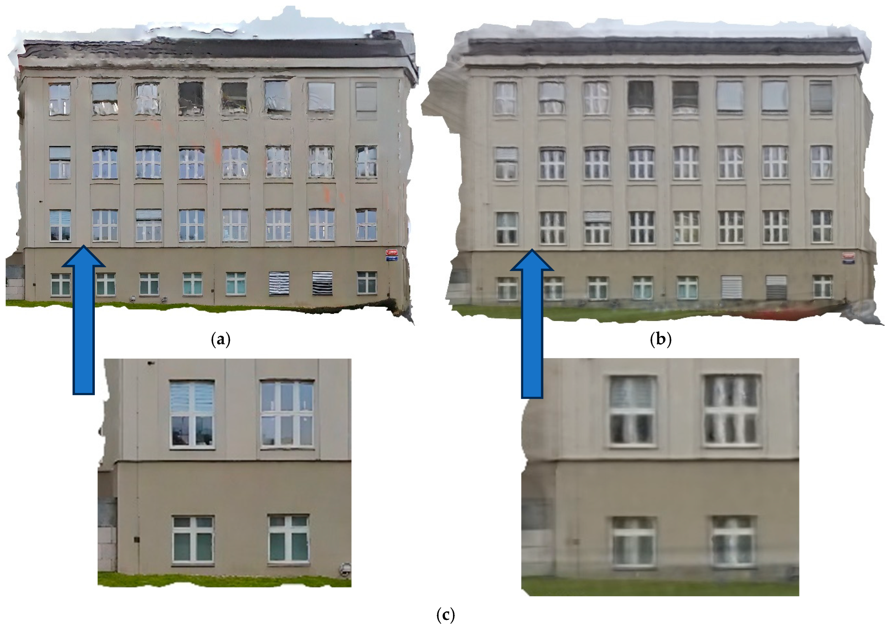Figure 6 shows the image before and after AI image editing. A very visible change is the unification of the plaster color and the highlighting of the edges of the window holes. Unfortunately, there is also deformation of some objects, as shown in the red circle.

2.6.4. Agisoft Metashape

Agisoft Metashape 2.1.1 is a very well-known and used software in the field of photogrammetry. Among many other functions, it can process spherical images using the SfM-MVS method.

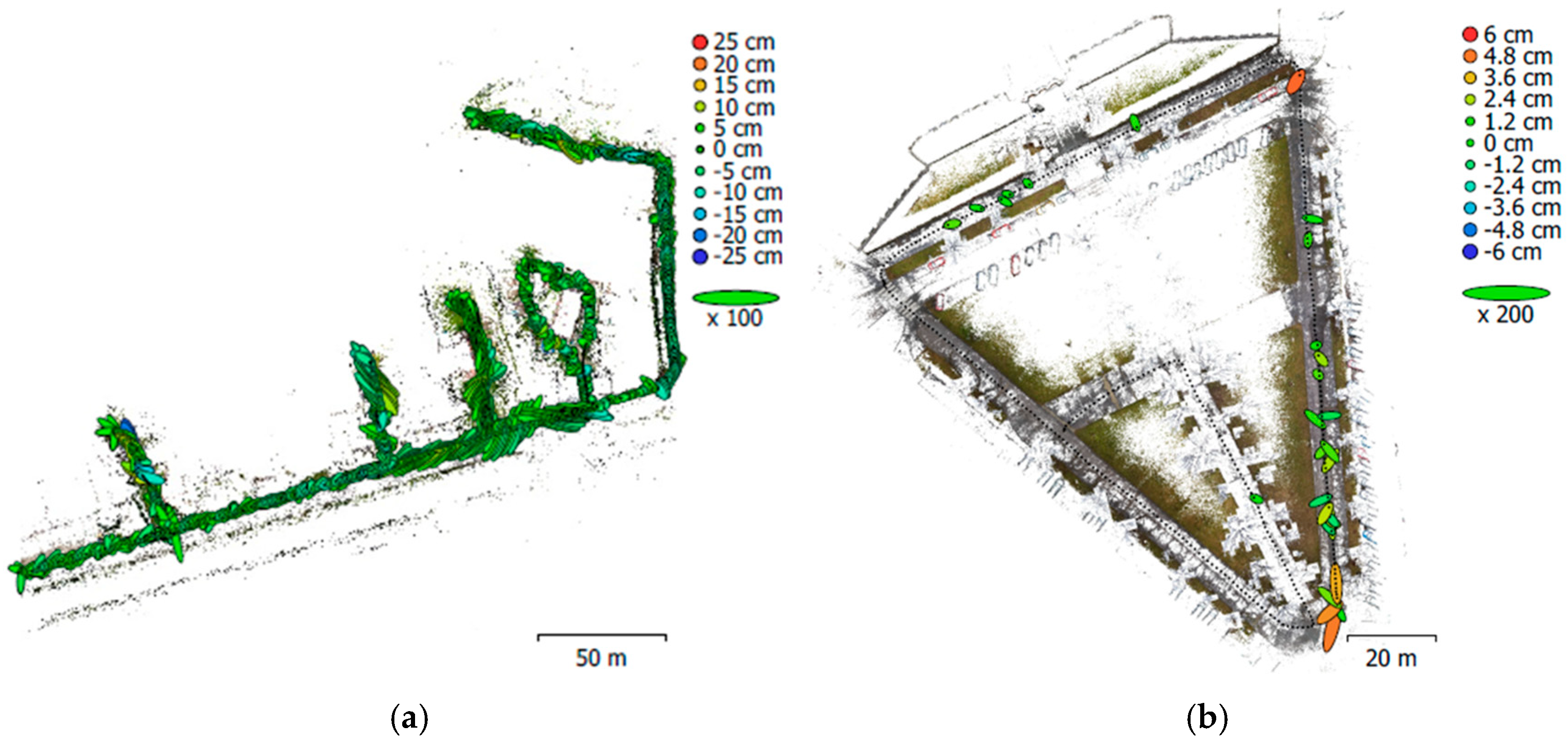
The type of camera-recorded images was set as spherical images. The images were masked so that the GNSS equipment was not included in the calculation. The basic alignment of the images was performed with the position of all images. This process produced a thin point cloud that contained the key points. However, the alignment of the thin point cloud was subsequently performed only with images containing a 3D position quality of less than 8 cm and on a few GCPs spread over the measured area. In Agisoft Metashape, GCPs were manually marked in images where the target center was clearly visible. Considering the spherical image resolution (5760 × 2880 px) and typical distances of 5–10 m, the ground resolution ranged from approximately 5 to 11 mm per pixel. Therefore, the target center was generally located with an estimated precision of 1–2 pixels, resulting in a real-world precision of about 0.5–2 cm. Only frames with a clear view were used for marking. Figure 7 shows the positions of the cameras, and, for the images for which their positions were used for alignment, the deviations are shown in the form of error ellipses.

The final step was to calculate the dense point cloud. Important parameters of the calculation, such as the processing time and accuracy at the ground control points, are listed in

Table 4. Agisoft Metashape processing parameters.

Case	Number of Images	Total Computation Time of Dense Point Cloud	St. Dev. X of GCPs [mm]	St. Dev. Y of GCPs [mm]	St. Dev. Z of GCPs [mm]	St. Dev. XYZ of GCPs [mm]
Fleming Square	406	6 h 30 min	22	6	39	46
Lipová street	1394	8 h 10 min	48	35	118	132

. Properties of the computing station: RAM—32GB; CPU—Intel i7-7700; and GPU—NVIDIA Quadro P1000S.

2.6.5. Accuracy Evaluation

For the calculations of relative accuracy and absolute accuracy, the formula of standard deviation for a single coordinate (1), for a plane (2), and for space (3) was used.

$$\begin{gathered} StDev=\sqrt{{\displaystyle \frac{{\sum }_{i=1}^n{v}_i^2}{n-1}}},where{v}_i=\Delta \underset{\_}{x}-{\Delta x}_i, \\ {\Delta x}_{i}representsthevalueofthei-thpointforthegivencoordinate\left(X,Y,Z\right), \\ \Delta \underset{\_}{x}isthemeanvalueforthegivencoordinate\left(X,Y,Z\right);nisthenumberofpoints \end{gathered}$$

(1)

$${StDev}_{XY}\mathrm{ }=\mathrm{ }\sqrt{\mathrm{ }\mathrm{ }{\displaystyle \frac{{\sum }_{i=1}^n{v}_{Xi}^2+v_{Yi}^2}{n-1}}}$$

(2)

$${StDev}_{XYZ}\mathrm{ }=\mathrm{ }\sqrt{\mathrm{ }\mathrm{ }{\displaystyle \frac{{\sum }_{i=1}^n{v}_{Xi}^2+v_{Yi}^2+v_{Zi}^2}{n-1}}}$$

(3)

3. Results

In this section, results from various methods of evaluating point cloud accuracy and quality are presented. First, the relative accuracy of the measured point cloud is evaluated by comparing the clouds; then, the section deals with the absolute accuracy of the measured cloud relative to the ground checkpoints measured by GNSS RTK. The last topic in this chapter is the evaluation of the quality of the data obtained from the Insta360 X3 camera. Here, the quality of the original data output is also compared with the AI-edited data.

3.1. Relative Accuracy and Deformation from Spherical Images

The cloud-to-cloud method was used to evaluate the relative accuracy and cloud deformation obtained from georeferenced spherical images from the Insta360 X3 camera. CloudCompare 2.13.1 [34] software was used for this purpose. The point clouds were aligned (congruent transformation) to several identical points, and the compute cloud/cloud distance function was run. Depending on the test, either full 3D (XYZ) distances or horizontal (XY) deviations were computed. The visualized errors correspond to the selected type and are shown in 2D views for clarity. The spatial standard deviation of the first point cloud compared to the Faro Orbis point cloud is 47 mm. In the second case, compared to the Mavic 3E point cloud, the spatial standard deviation reaches 82 mm. The resulting standard deviations are presented in

Table 5. Cloud-to-cloud standard deviations.

Case	St. Dev X [mm]	St. Dev Y [mm]	St. Dev Z [mm]	St. Dev XY [mm]	St. Dev XYZ [mm]
Fleming Square	25	26	32	37	47
Lipová street	33	35	65	41	82

.

The following figures provide a top view of the measured test area with histograms showing the magnitude of the deviations produced from the point cloud differences. Figure 8 shows the 2D deviations, and Figure 9 focuses on the 3D deviations. The 3D deviation charts of the Lipová street test site are the most different here, and there is a significant error in the Z-axis direction. This may be due to the lower accuracy of the reference point cloud than is present in the Fleming Square test site.

Figure 7. Camera positions and deviations: (a) case study of Lipová street; (b) case study of Fleming Square.

Figure 7. Camera positions and deviations: (a) case study of Lipová street; (b) case study of Fleming Square.

3.2. Absolute Accuracy

To evaluate the cloud’s absolute accuracy, i.e., against the coordinate system, identical points were taken from the computed point clouds, and these were compared with the reference points.

Table 6. Standard deviations of absolute accuracy.

Case	St. Dev X [mm]	St. Dev Y [mm]	St. Dev Z [mm]	St. Dev XY [mm]	St. Dev XYZ [mm]
Fleming Square	53	64	55	83	99
Lipová street	56	61	-	83	-

shows these point cloud accuracies. The 2D accuracy was found to be the same for these test areas, reaching 83 mm in both cases. As mentioned above, the reference points for the Lipová street case study were only 2D, so the height component could not be evaluated here. Figure 10 shows the deviations of the individual points using error ellipses.

3.3. Quality of Processed Data

Data quality was assessed in several ways. First, it was compared with the quality of the reference methods.

Table 7. Number of points in selected parts.

Case	Reference Point Cloud	Insta360 X3 Point Cloud
Fleming Square—facade	3,871,009 points	665,936 points
Lipová street—a single parcel	2,864,192 points	2,130,744 points

shows the number of points in the point cloud section. The final number of points in the cloud facade on Fleming Square from the computed spherical images is more than 6 times lower than that from the SLAM method. The quality of the facade can also be seen in Figure 11, and significant features were captured. This is also reflected in the quality of the model (Figure 12), where a more significant deformation of the model occurs on higher floors of the building.

In the case study of Lipová street, the data quality is already comparable to the reference (Table 7), and visibly (Figure 11), the data are better. This may be because all parts of the building were walked “forward and back” with the device.

The point cloud of the facade created from the AI-edited images, using a pre-trained realesrnet-x4plus model, had a very similar accuracy to the facade from the original images. The only significant difference is in the texture of the models. Figure 12 shows the orthophotos of the facade. Both images show the cloud deformation that occurs on the upper floors of the building. More significant deformations are seen in the orthophoto with the AI-modified images. The deformations are very similar in both examples, and only in the model with the original photos are they more blurred. At first glance, the AI orthophoto is significantly sharper and more engaging, especially on the first two floors. The difference in the quality of the lower and higher floors of the facade is not only due to the higher distortion, which increases with the distance from the center of the fisheye lens, but also because part of the upper floors was partially covered by the GNSS equipment when passing close to the facade.

The pre-trained ESRGAN model used is not trained to work with spherical images, and therefore, one way to improve AI-edited images and create orthophotos would be to re-train it on its own dataset.

To prevent deformation of the upper floors, with both types of images, we can choose from several options:

• Sensing from a greater distance—this will affect the spatial resolution of the façade.
• Sensing from the same distance, but the camera and GNSS are placed at a higher elevation on the pole.
• Setting a more extensive mask when processing the model, so that when passing close to the facade, parts of the image with high distortion are not used.
• Adding images without using GNSS and without obscuring the top of the images.
• Combining the above methods.

3.4. Experimental Verification

To verify the proposed improvements, an experiment was conducted where selected methods were tested. In this experiment, a combination of the suggestions from the previous section was carried out. First, a series of images was taken at ca. 10 m from the façade; the camera height was 2 m above the surface in the first pass and 4 m in the second pass. Following this, without GNSS equipment, images were taken at two equal height levels (2 and 4 m) at 3 m from the facade. A comparison of this experiment with the point cloud from Faro Orbis is shown in Figure 13.

4. Discussion and Conclusions

The results of this paper indicate that a mapping device made from a commercially available action camera and low-cost GNSS equipment is a suitable tool for mapping outdoor areas, of course with a given degree of accuracy. However, for this purpose, accurate synchronization of the spherical camera and GNSS clocks is required. For this purpose, the 360VisualSync software was developed and tested together with the constructed device.

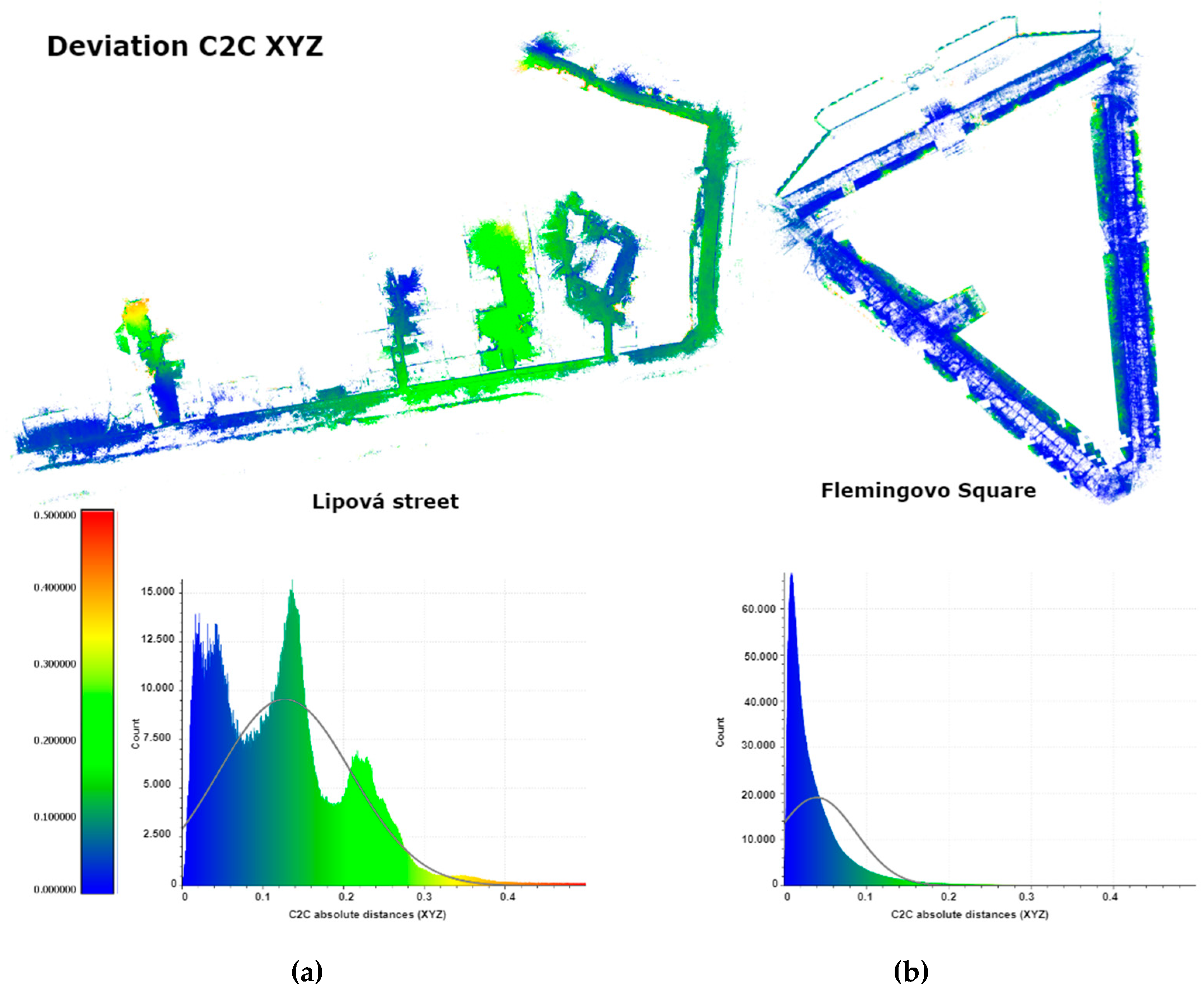
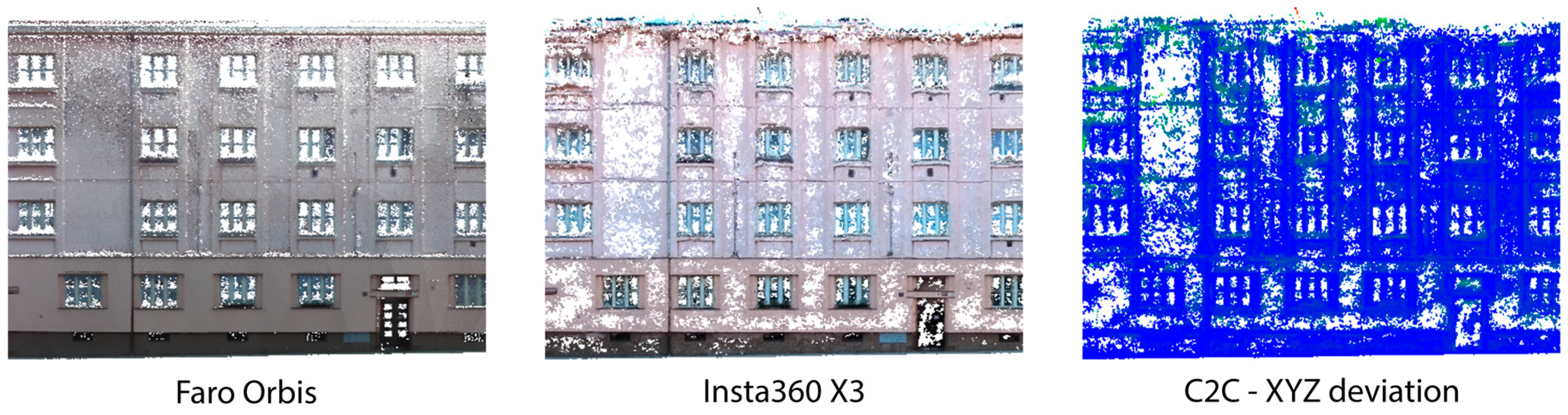
The first test was carried out on a square with trees and surrounded by urban buildings. Measurements were compared with the SLAM method using the Faro Orbis device. The spatial accuracy of the low-cost method, determined by comparing point clouds here, was 47 mm. The absolute spatial accuracy was then evaluated using ground GNSS RTK points, and, in this case, a spatial standard deviation value of 99 mm was found.

The second test site was on Lipová street in Kopidlno. Here, a housing development with detached houses was surveyed. The point cloud was first compared with the point cloud calculated from the images from the Mavic 3E drone. Although the plane’s standard deviation was very similar to the previous test, in this case, the spatial standard deviation of the difference between the point clouds was significantly higher, at 82 mm. This may have been due to the accuracy of the reference point cloud. The absolute reference points used here were independently determined by the Cadastral Office. The standard deviation of this comparison was identical to the first test, at 83 mm.

Compared to the work of [13], where the absolute 2D standard deviation achieved was between 17 and 20 cm, the precision achieved in this article is 2 times higher.

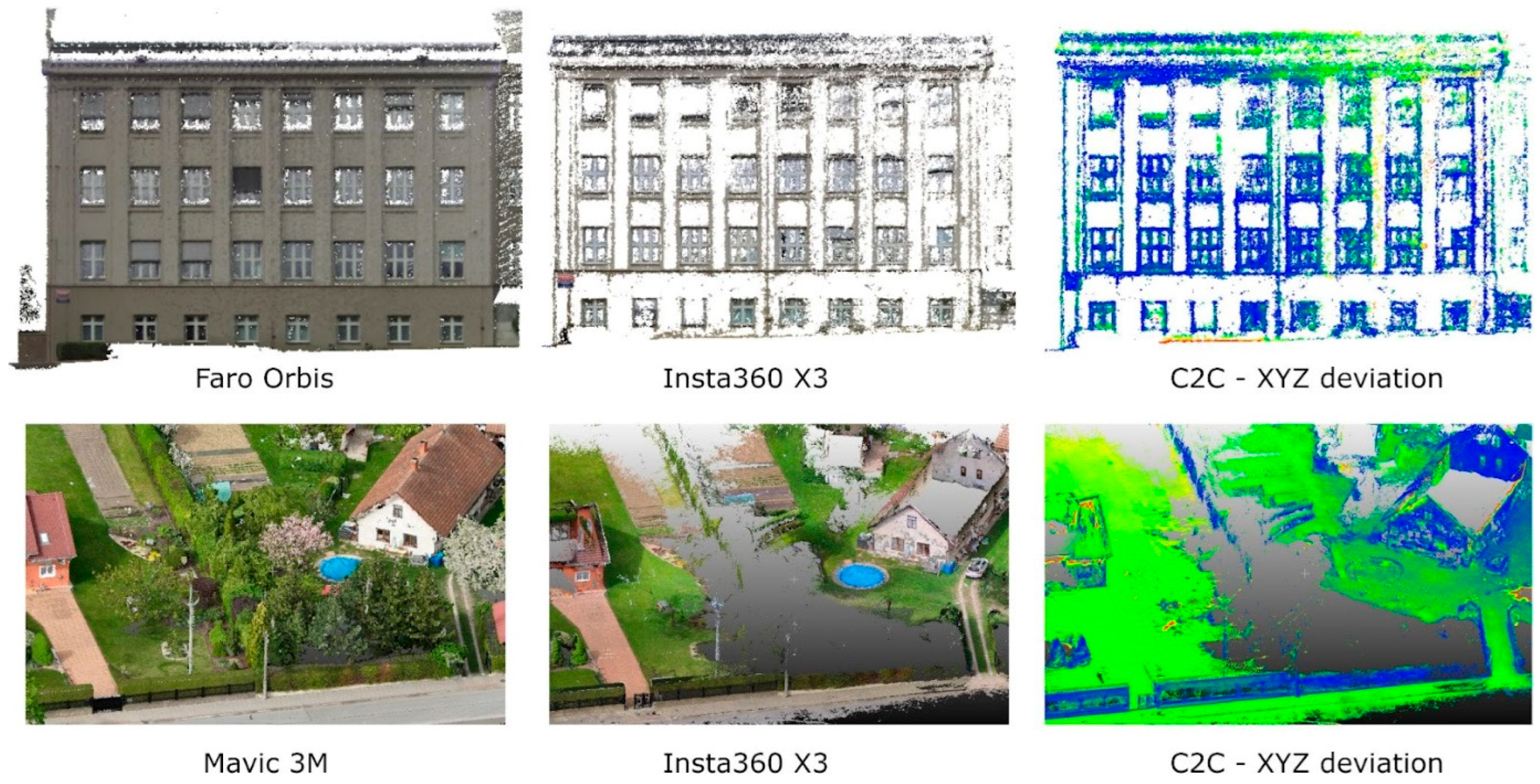
Finally, the products were evaluated in terms of data quality. In general, in photogrammetry, a common problem is the evaluation of simple single-color objects. This was also reflected in this case, especially for the facade from the first test, where only distinctive elements, such as windows, were calculated with sufficient confidence. The point cloud from the second testing is of significantly higher quality. When measuring this area, each section was walked “back and forth”. Following the results of the data quality of the house facade capture, several procedures were proposed to improve the quality of the measurements. These suggested approaches were then verified in an experiment. The results from this experiment show an improvement in the quality and density of the facade point cloud. Unfortunately, as in the previous case, there is a noticeable deformation in the higher parts of the facade.

The processing of spherical images with the Real-ESRGAN machine learning tool, designed to increase the resolution of the images, did not produce significant changes in the accuracy of the point cloud or its density. The texture quality of the model and orthophoto are greatly affected by the modified images, with results that are sharper and of higher visual quality than when processed with the original images. Using these edited images also makes deformations in the orthophoto, which are otherwise hidden behind the lower quality of the captured data, more noticeable.

The quality of the resulting point clouds proved to be highly dependent on several parameters: the distance between the camera and the object (typically 3–10 m), the interval of frame extraction (1 s), the operator’s walking speed (around 4–5 km/h), and the GNSS signal quality. These factors directly influenced the density, sharpness, and geometric consistency of the reconstructed point cloud.

Sharp object edges, repetitive textures, and strong contrast improved the reliability of point matching, whereas uniform or single-color surfaces often led to missing areas or deformations. Significant errors were observed when the operator walked too close to the facade or when objects were partly occluded by the GNSS antenna.

With the knowledge of these results, it can be said that the device is suitable for mapping objects where the required accuracy is between 5 and 10 cm. The major advantage of this device is its very low price, which is around EUR 1000. The price of the Faro Orbis mobile scanner is around EUR 60,000.

The usefulness of this equipment is therefore especially beneficial for quick and cheap surveying of smaller sites, especially in smaller villages, and for teaching, where this equipment can be easily and cheaply implemented into basic teaching of surveying and mapping. Major limitations of the current workflow include the need for manual time synchronization between the GNSS track and video frames, which may introduce errors if not performed precisely. In environments with degraded GNSS signals, such as narrow streets or under vegetation, the absence of additional sensors can lead to unstable or inaccurate trajectories. The final disadvantage of this methodology is the difficulty of data processing. A user educated in photogrammetry is needed to evaluate the images.

Future work could focus on improving the quality of the measured data by adding additional equipment to take photos of better quality than images from videos or small laser scanners. It would also be useful to create a device with professional GNSS equipment or to improve the position using data from the camera gyroscope.