Multi-Objective Optimal Allocation of Regional Water Resources Based on the Improved NSGA-III Algorithm

Abstract

Rapid socio-economic development has intensified the conflict between supply and demand for regional water resources, necessitating optimized water resource allocation to enhance water security. This study establishes a multi-objective water resource optimization model by comprehensively considering economic, social, and ecological benefits. Based on the Non-dominated Sorting Genetic Algorithm-III (NSGA-III), we propose the I-NSGA-III algorithm by integrating reference point improvement strategies, dynamic retention of high-quality solutions, and optimized selection strategies to solve the multi-objective optimization model. A multi-system coupling coordination evaluation model is constructed to assess the final allocation schemes. Compared with some commonly used multi-objective algorithms and tested using the DTLZ series functions, the proposed algorithm demonstrates improved overall performance. Specifically, the IGD indicator decreases by 5.17–50.22%, and the HV indicator increases by 2.71–25.51% compared to NSGA-III. The proposed model is applied to Jinzhong City, China, with four scenarios set for the years 2030 and 2035 at P = 50% and P = 75% to derive reasonable water resource allocation schemes. The results show that the economic benefits range from 161.94 × 10⁸ to 212.74 × 10⁸ CNY, the water shortage rate is controlled between 1.38% and 10.86%, and COD emissions are maintained between 6.03 × 10⁴ and 6.91 × 10⁴ tons. Except for the 2030 drought scenario (P = 75%) with a coordination degree of 0.7847, classified as a medium coordination level, all other scenarios have coordination degrees greater than 0.8, indicating a good coordination level. The optimized allocation scheme can serve as a reference for the rational allocation of water resources in Jinzhong City. Moreover, the method proposed in this paper is a general approach that can be extended to other similar water-scarce cities with appropriate parameter adjustments, contributing to the sustainable development of urban water resources.

1. Introduction

As a critical element for sustaining ecological balance and supporting socio-economic development, the rational allocation of water resources constitutes the central challenge in achieving regional sustainable development [1,2]. The interplay of global climate change, urbanization, and rapid economic growth has exacerbated the imbalance between water supply and demand, while issues such as water pollution and the degradation of aquatic ecosystems have become increasingly prominent [3,4,5,6]. This situation is particularly severe in northern China. For example, in Jinzhong City, Shanxi Province, 2023 statistical data reveal that its per capita water availability falls below one-fifth of the national average, with intense competition between industrial and agricultural water use, and ecological baseflows are difficult to maintain [7,8]. Therefore, under the constraint of limited total water resources, devising scientifically sound allocation strategies to meet the diverse water demands of society and the economy has become a pressing issue in water resource management.

Water resource optimization, as a critical technical approach for sustainable water management, is characterized by multi-dimensional coupling, dynamic interactions, and spatial heterogeneity. Its core lies in constructing multi-objective optimization models to seek Pareto-optimal solutions within complex solution spaces defined by resource constraints, competitive user demands, and ecological redlines. Since the 1970s, academia has gradually established a theoretical framework for water resource system analysis, marked by Haimes’ multi-objective decision-making framework [9,10] and Loucks’ stochastic programming models [11], forming a technical pathway of “system modeling-scenario simulation–solution prioritization.” In the early stages of research, water resource allocation typically focused on single-objective optimization targeting economic benefits, using methods such as linear programming [12] and dynamic programming [13]. These single-objective models did not consider social and ecological factors, lacking the capacity for comprehensive water resource development and utilization.

As research has progressed, water resource optimization has shifted from pursuing a single objective to maximizing the comprehensive benefits of multiple objectives. Consequently, water resource system modeling has evolved from linear programming to mixed-integer nonlinear programming, with solution algorithms undergoing multiple transformations: initially, classical algorithms like the simplex method and dynamic programming laid the computational foundation; in the intermediate phase, intelligent algorithms, such as genetic algorithm (GA) [14,15], particle swarm optimization algorithm (PSO) [16,17], and simulated annealing algorithm (SA) [18,19], were introduced to address high-dimensional non-convex problems; currently, we are in a phase of multi-algorithm integration and innovation, with multi-objective optimization algorithms, like the non-dominated sorting genetic algorithm-II (NSGA-II) [20], multiple objective particle swarm optimization (MOPSO) [21], and multi-objective evolutionary algorithm based on decomposition (MOEA/D) [22], gaining attention for their advantages in solving complex multi-objective optimization problems and being widely used in multi-objective water resource optimization studies. It is worth noting that, in recent years, such algorithms have been practically validated in typical regions of Shanxi Province. Liu et al. [23] proposed a hybrid algorithm that integrates NSGA-II with an Adaptive Real-coded Simulated Binary Crossover (ARSBX) strategy for the optimal allocation of water resources in Taiyuan City. The resulting scheme achieved a coordination degree exceeding 0.8, significantly alleviating the city’s water scarcity. Li et al. [24] improved the inertia weight and learning factors of the Particle Swarm Optimization (PSO) algorithm and applied it to the optimal allocation of water resources in Yangquan City. The resulting water-saving scheme not only mitigated water shortages across administrative districts but also reduced COD emissions, thereby easing ecological and environmental pressures.

When solving multi-objective optimization allocation models for water resources using multi-objective optimization algorithms (MOAs), a series of non-dominated solution sets are obtained instead of a single optimal solution, due to the characteristics of multi-objective optimization problems. Therefore, to ensure the scientific and rational allocation of water resources, evaluation methods are needed to filter the non-dominated solution sets in order to find the optimal solution that maximizes overall benefits. Common evaluation methods include the analytical hierarchy process (AHP) [25], the entropy weight method [26], and the technique for order preference by similarity to ideal solution (TOPSIS) [27]. The AHP relies heavily on expert experience for weighting, making it quite subjective. The Entropy Weight Method calculates weights based on data distribution, offering more objectivity, yet it fails to reflect decision-makers’ preferences and is highly sensitive to the distribution of the indicators’ data. TOPSIS is a ranking method based on distance measurement, but it lacks the ability to evaluate the synergy between multiple systems, making it difficult to fully reflect the comprehensive effects of water resource allocation. The coupled coordination degree evaluation model [28] is constructed based on system theory and synergy theory. Its advantages lie in quantifying the feasibility of comprehensive benefit evaluation schemes on the one hand and analyzing the interactive coupling relationships between multiple systems to determine whether the schemes meet the requirements for coordinated development on the other. Compared to traditional evaluation methods, this model overcomes the shortcomings of single evaluation dimensions and insufficient representation of dynamic correlations. It can quantitatively represent the overall coordination of water resource allocation schemes under multi-objective constraints, making it suitable for indicator evaluation in water resource optimization allocation.

Furthermore, as mentioned above, NSGA-III, as a representative algorithm in the field of multi-objective optimization, demonstrates excellent convergence and distribution, showing significant advantages in solving multi-objective optimization problems [29]. However, the NSGA-III algorithm can only generate a series of reference points through pre-definition and, in actual multi-objective optimization problems, the true Pareto front (PF) is often unknown in advance, so the preset reference points may not reflect the development trend of the PF. To address this issue, this study proposes three improvements: reference point improvement strategy, adaptive solution retention mechanism, and Pareto front screening strategy, to construct an improved NSGA-III (I-NSGA-III) algorithm. The improved I-NSGA-III is applied to the southern water supply zone of Jinzhong City, providing a diverse set of alternative solutions for water resource optimization and offering theoretical support and methodological innovation for water resource optimization in water-scarce northern regions.

2. Construction of a Water Resource Optimization Model

2.1. Objective Function

The fundamental goal of water resource optimization is to achieve efficient utilization of regional water resources and ensure sustainable regional development. Based on this premise, the model in this paper aims to maximize economic benefits, minimize the total regional water shortage, and reduce pollutant emissions as its objective functions.

(1)

Economic Objective: The objective function is to maximize the water supply benefits.

$$f_1(x)=max\sum _{k=1}^K[\sum _{j=1}^J\sum _{i=1}^I(b_j^k-c_j^k)x_{ij}^k{a}_i{\lambda }_j]$$

(1)

In the formula, k represents the water supply sub-region. i denotes water supply sources, categorized into surface water, groundwater, transferred water, and reclaimed water. j represents water users, classified as domestic, production (primary, secondary, and tertiary industries), and ecological; $b_j^k$ and $c_j^k$ are the water supply benefit coefficient and cost coefficient for water user j in supply sub-region k, Unit: CNY; $a_i$ is the water supply priority coefficient for water source i; ${\lambda }_j$ is the water use equity coefficient for water user j; $x_{ij}^k$ is the water allocation volume from water source i to water user j in supply sub-region k, Unit: 10⁴ m³.

(2)

Social objective. The objective function is to minimize the total water shortage of water users.

$$f_2(x)=min\sum _{k=1}^K[\sum _{j=1}^J\sum _{i=1}^I(D_j^k-x_{ij}^k)]$$

(2)

In the formula, $D_j^k$ represents the total water demand of water user j in supply sub-region k, Unit: 10⁴ m³.

(3)

Ecological and Environmental Objective: The objective function is to minimize the pollutant emissions.

$$f_3(x)=min[\sum _{k=1}^K\sum _{j=1}^J{\alpha }_j^k{\beta }_j^k(\sum _{i=1}^I{x}_{ij}^k)]$$

(3)

In the formula, ${\alpha }_j^k$ is the Sewage Discharge Coefficient for water user j in supply sub-region k; and ${\beta }_j^k$ represents the pollutant discharge concentration for water user j in supply sub-region k, Unit: mg/L.

2.2. Constraints

When addressing the multi-objective optimization of water resource allocation, it is essential to consider various constraints, including water demand and water supply. Solutions that satisfy these constraints are the only ones that hold practical significance. The constraints selected in this study include water availability constraints, water demand constraints, pollutant emission constraints, and non-negativity constraints for variables.

(1)

Water Availability Constraint:

$$max\sum _{k=1}^K\sum _{i=1}^I\sum _{j=1}^J{x}_{ij}^k\le W_i^k$$

(4)

In the formula: $W_i^k$ represents the maximum available water supply from water source i in supply sub-region k.

(2)

Water Demand Constraint

$$D_{jmin}^k\le \sum _{i=1}^I\sum _{j=1}^J{x}_{ij}^k\le D_{jmax}^k$$

(5)

$$D_{jmin}^k={\mathrm{\epsilon }}_j^k\times D_{jmax}^k$$

(6)

In the formula: $D_{jmax}^k$ represents the upper limit of water demand for water user j. $D_{jmin}^k$ represents the lower limit of water demand for water user j. ${\mathsf{\varepsilon }}_j^k$ is the minimum water supply guarantee rate for water user j in supply sub-region k.

(3)

Pollutant discharge limit constraint:

$${\alpha }_j^k{\beta }_j^k\times \sum _{i=1}^I{x}_{ij}^k\le Q_j^k$$

(7)

In the formula: $Q_j^k$ represents the maximum allowable discharge concentration of local water pollutants in supply sub-region k. ${\alpha }_j^k$ is the sewage discharge coefficient in the effluent of water user j in supply sub-region k; ${\beta }_j^k$ represents the pollutant discharge concentration in the effluent of water user j in supply sub-region k.

(4)

Non-negativity constraint on variables:

When addressing real-world problems, all referenced variable values must be guaranteed to be non-negative.

3. Algorithm Improvement and Scheme Evaluation

3.1. Improvement Strategy for the NSGA-III Algorithm

The basic framework of the NSGA-III algorithm is similar to that of the NSGA-II algorithm, but its mechanisms have undergone significant changes [30]. NSGA-II maintains population diversity through crowding distance, focusing on preserving the physical distance between solutions. However, as the number of objectives increases, mere distance calculation is insufficient to fully capture the diversity among solutions. NSGA-III addresses this limitation by introducing reference points. During the algorithm’s initialization phase, a set of uniformly distributed reference points is generated to guide the population’s development direction in subsequent evolutionary processes. By calculating the proximity of individuals to these reference points—typically using normalized Euclidean distance or angular distance—representative individuals are selected to advance to the next generation. This approach enables the algorithm to explore complex Pareto frontiers composed of multiple objectives. However, in practical multi-objective optimization problems, fixed reference points cannot reflect the dynamic changes of the true Pareto frontier, leading to ineffective reference points that interfere with the evolution of population individuals. To address this issue and make the algorithm more adaptable to constrained multi-objective optimization problems, adjustments are necessary. This paper improves the algorithm in three aspects: Reference point improvement Strategy, Dynamic Solution Retention Mechanism, and optimization selection strategies.

3.1.1. Reference Point Improvement Strategy

Before applying the NSGA-III algorithm, a set of reference points must be provided [31], which serves to guide the population towards the Pareto-optimal front (PF). Traditional algorithms, such as those proposed by Das and Dennis [32], generate a set of fixed reference points at predefined positions on a normalized hyperplane. However, the distribution of the PF in real-world problems is often unknown, and fixed reference points may fail to adapt to dynamic changes during the optimization process. As a result, they may not accurately reflect the true evolution of the PF. To address this issue, we introduce an adaptive reference point generation method based on population information. This method produces a set of reference points that perform well in terms of both convergence and distribution. However, the introduction of new reference points increases the total number of reference points, which can elevate the computational complexity of the algorithm. To mitigate this, we introduce a reference point elimination mechanism to maintain the algorithm’s convergence speed.

(1) Generating New Reference Points:

In the traditional NSGA-III algorithm, after niche operations, the population $P_{t+1}$ is generated, and the niche counts α for different reference points are updated, with the initial niche count for all reference points set to α = 1. If the h-th reference point is not associated with any population members, its niche count α_h is set to zero. These unassociated reference points are considered ineffective for exploring the current PF and are termed “ineffective reference points”. In such cases, it is optimal to replace the h-th reference point with a new one to better reflect the direction of the PF. Under these conditions, Formulas (8) and (9) are used to introduce a set of new reference points, with the number of new reference points being equal to the number of ineffective (α = 0) reference points.

$$h_{new}^g=\underset{x\in P_t}{min}{f}_g(x)+{\epsilon }_g$$

(8)

$${\epsilon }_g=\delta \left(f_g^{max}-f_g^{min}\right)$$

(9)

In the formula, $P_t$ is the parent population of the t-th generation (size N), x is the individual in the population $P_t$, δ is a random number uniformly distributed in (0, 1), $h_{new}^g=(h_{new}^1,h_{new}^2,\cdots ,h_{new}^G)$ represents the new reference point of the target g, $f_g^{max}$ and $f_g^{min}$ are the maximum and minimum values of the target g, respectively.

(2) Elimination of Invalid Reference Points:

As new reference points are dynamically added, the total number of reference points increases significantly, thereby raising the computational burden of the algorithm. To address this issue, after each iteration, the niche count α for all reference points is recalculated and recorded. The total niche count α is set equal to the population size N (i.e., ${\sum }_{h=1}^H{\alpha }_h=N$). Ideally, each reference point should be associated with exactly one solution in the population $P_{t+1}$. Subsequently, all reference points with α = 0 are removed from the set of reference points H. To maintain a uniform distribution of reference points, the original reference points generated by the method of Das and Dennis [32] are always retained. This ensures that the reference points remain systematic and consistent. Consequently, the set of existing reference points consists of two parts: the original reference points (even those with α = 0) and all newly added reference points with α = 1.

3.1.2. Dynamic Solution Retention Mechanism

To enhance the convergence speed of the NSGA-III algorithm in the early iteration stages, this paper proposes a probabilistic mechanism to retain the solution closest to the ideal point, aiming for faster convergence in the initial phase.

The implementation is as follows: During the first 25% of the evaluation count in population evolution, this retention strategy is triggered with a random probability of 50%. Each time it is triggered, the set of objective values for all individuals in the population that meet the constraint conditions is recorded as matrix M. The Euclidean distance from each individual to the current ideal point Z is then calculated (Equation (10)). The ideal point Z is determined by calculating the minimum value of each objective function, resulting in $Z(x_{min},y_{min},\dots ,z_{min})$. Based on this, the individual q in the population closest to the ideal point Z is identified using a minimum distance search method and marked as the retained solution. In the subsequent environmental selection phase, this solution q is prioritized for entry into the next generation population to strengthen the algorithm’s early convergence capability.

For two points $A(x_1,x_2,\dots ,x_n)$ and $B(y_1,y_2,\dots ,y_n)$ in an n-dimensional space, the Euclidean distance (d) is given by the following formula:

$$d=\sqrt{\sum _{i=1}^n(y_i-x_i{)}^2}$$

(10)

In the formula, $x_i$ and $y_i$ represent the coordinate values of points A and B in the i-th dimension, respectively.

3.1.3. Optimization of Selection Strategy

In the traditional NSGA-III algorithm, the tournament selection strategy randomly selects candidate individuals for comparison. A fixed number of individuals are chosen in each round and, through comparing the dominance relationships among individuals, the superior ones are selected to enter the mating pool. Although this method considers the non-dominated rank of individuals during selection, it does not dynamically control the number of candidates and the diversity of individuals. This may lead to insufficient early convergence of the population or local convergence due to poor individual quality. To address these issues, this paper proposes an adaptive tournament selection strategy with the following key improvements.

(1) Dynamic Adjustment of Candidate Number:

In each round of tournament selection, the number of candidate individuals K is dynamically adjusted based on the number of individuals in the first non-dominated front (i.e., the Pareto front) of the population, in order to accelerate the selection of high-quality individuals. The specific calculation method is as follows:

$$K=\lceil {\displaystyle \frac{FN}{3}}\rceil$$

(11)

Here, FN represents the number of individuals currently in the first non-dominated front of the population, and $\lceil *\rceil$ denotes the ceiling operation. By dynamically adjusting the value of K, the strategy can prioritize the retention of superior individuals in the early stages of evolution, aiding the population in exploring better solutions early on and enhancing the overall quality of the population.

(2) Priority Selection Based on Non-Dominated Sorting:

Among the randomly selected K candidate individuals, sorting is performed based on their non-dominated ranks. The individual with the lowest non-dominated rank is prioritized as the winner, enabling the population to quickly converge towards the Pareto front.

3.1.4. Algorithm Implementation Process:

Step 1: Population Initialization. Randomly generate an initial population P_t (where (t = 0)) consisting of N individuals according to the constraints. Then, calculate the objective function values for each individual in the population and perform a fast non-dominated sorting on all individuals.

Step 2: Calculation of Ideal and Reference Points. Determine the ideal point Z by calculating the minimum value for each objective function and define a series of reference points H according to the conditions. Then evaluate the association degree between each individual i in the population and the reference points.

Step 3: During the first 25% of evaluation counts in population evolution, the dynamic solution retention mechanism used in this paper is employed to select and mark excellent individuals, which then directly participate in the subsequent population evolution.

Step 4: Selection of Parent Population. Use the adaptive tournament selection strategy proposed in this paper to screen and compare individuals in P_t, selecting the best-performing individuals to construct the next generation’s parent population.

Step 5: Generation of Intermediate Population. Obtain a new offspring population Q_t through crossover and mutation operations on the parent population. Then, merge the parent population P_t with the offspring population Q_t to form the intermediate population C_t, which includes all members of P_t and Q_t.

Step 6: Selection of High-Quality Solutions. Perform non-dominated sorting on the population C_t to select outstanding individuals to join the population P_t+1. During the first 25% of evaluation counts in population evolution, use the dynamic solution retention mechanism proposed in this paper to select excellent individuals to join P_t+1.

Step 7: Dynamic Adjustment of Reference Points. Create the population P_t+1 through niche operations at the final stage of the selection process. If there are invalid reference points, dynamically adjust the reference points H according to the reference point improvement strategy proposed in this paper.

Step 8: Iteration Termination Criterion. Increment t by 1. If t exceeds the predefined limit T_m, terminate the iteration process and consider the non-dominated solutions in the current population P_t as the Pareto optimal set. If t has not yet reached T_m, return to Step 2 and continue the process.

The pseudo code of the Algorithm 1 is as follows:

Algorithm 1: Pseudo-code of I-NSGA-III

1: Input: P0, Tm, N, H (Initial population, maximum number of iterations, Population size, reference point set) 2: Output: Pareto solutions 3: Initialize uniform distribution reference points H; t = 0; 4: Compute Zmin from feasible solutions in P0; 5: 6: while termination conditions are not satisfied (t < Tm) do 7: 8:       if t < Tm/4 and rand () < 0.5 then 9:             Use Improvement 1 to identify and reserve elite solution q; 10:             g = 1; (Indicates that a high-quality solution is selected) 11:       else 12:             g = 0; 13:       end if 14: 15:       (Section 3.1.3. Optimization of Selection Strategy) 16:       Perform non-dominated sorting on Pt; 17:             Use Improvement 2 to dynamically adjust selection Number of candidate individuals K; 18:       ζ= adaptive tournament selection (Pt, g); 19: 20:       Qt = Recombination & Mutation(ζ); 21:       Ct = Pt ∪ Qt; 22:       Perform non-dominated sorting on Ct; 23:       Pt+1 = SelectSolutions (Ct, g); 24: 25:       if g > 0 then 26:       Add reserved elite solution q to Pt+1; 27:       end if 28: 29:       Use Reference Point Improvement Strategy (Section 3.1.1) to generate new reference points based on current front; 30:       Update reference point set H; 31: 32:       t = t + 1; 33: 34:             end while 35: 36:       return Non-dominated solutions in Pt as Pareto-optimal front

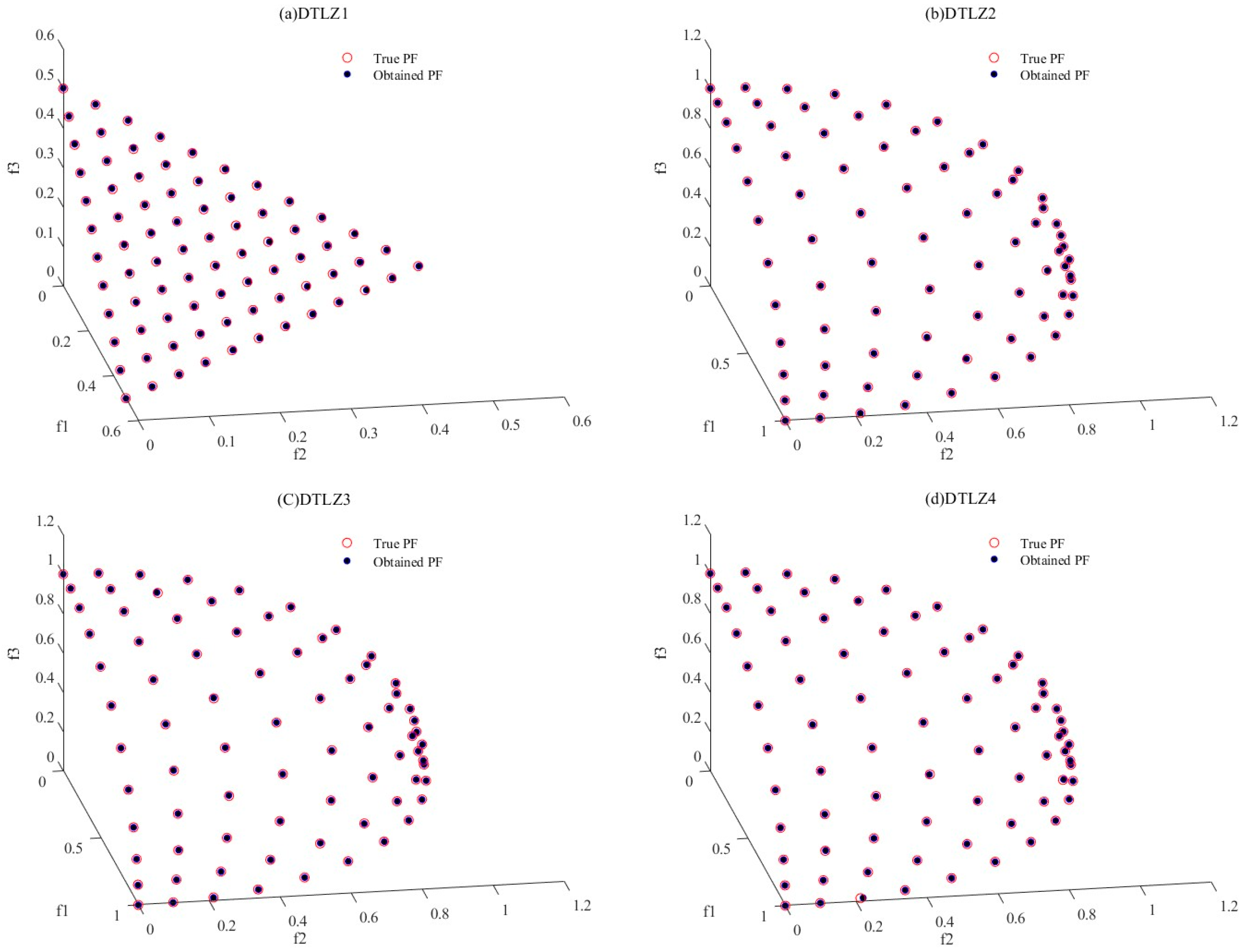
3.1.5. Algorithm Testing

To evaluate the overall performance of the I-NSGA-III algorithm, a systematic validation was conducted using the DTLZ standard test suite (DTLZ1-DTLZ4) proposed in reference [33]. The population size for all algorithms was set to 70, the number of objectives was set to 3, and the maximum number of iterations is referenced in

Table 1. Main features of test problems.

Function	Characteristics	Maximum Iteration
DTLZ1	Linear, multimodal	200
DTLZ2	Concave	500
DTLZ3	Concave, multimodal	700
DTLZ4	Concave, biased	400

. A comparison of the Pareto front obtained by I-NSGA-III for the DTLZ test problems with the true Pareto front of the test problems is shown in Figure 1. The results indicate that the solutions obtained by I-NSGA-III for the DTLZ test problems generally converge to the true Pareto front, demonstrating the feasibility of the I-NSGA-III algorithm.

To further validate the performance of the I-NSGA-III algorithm, two test metrics were used to evaluate I-NSGA-III, and comparisons were made with the NSGA-III, NSGA-II, MOEA/D and RVEA multi-objective algorithms. The test metrics are as follows: the Inverted Generational Distance (IGD) metric, where a smaller value indicates better overall algorithm performance [34]; and Hypervolume (HV), where a larger value indicates better convergence and diversity [35]. The main characteristics of all benchmark problems are shown in Table 1. To mitigate the effects of randomness, each algorithm was independently run 20 times on each test problem. The mean and standard deviation of each metric were calculated for comparison.

Table 2. Convergence result of three algorithms.

Function	Model	IGD		HV
		Median	Std.	Median	Std.
DTLZ1	I-NSGA-III	6.26 × 10−4	1.01 × 10−3	8.31 × 10−1	1.47 × 10−1
	NSGA-III	1.26 × 10−3	1.15 × 10−3	8.09 × 10−1	2.86 × 10−1
	NSGA-II	3.17 × 10−2	1.07 × 10−3	7.82 × 10−1	3.25 × 10−1
	MOEA/D	2.20 × 10−2	8.56 × 10−2	7.93 × 10−1	2.73 × 10−1
	RVEA	2.78 × 10−2	1.57 × 10−1	8.02 × 10−1	1.76 × 10−1
DTLZ2	I-NSGA-III	2.72 × 10−4	3.99 × 10−5	5.71 × 10−1	1.06 × 10−5
	NSGA-III	2.87 × 10−4	7.27 × 10−5	5.41 × 10−1	1.88 × 10−5
	NSGA-II	8.62 × 10−2	4.41 × 10−3	5.18 × 10−1	3.98 × 10−1
	MOEA/D	2.75 × 10−4	2.76 × 10−4	5.51 × 10−1	1.21 × 10−5
	RVEA	2.45 × 10−4	4.26 × 10−5	5.51 × 10−1	7.64 × 10−5
DTLZ3	I-NSGA-III	1.36 × 10−2	1.42 × 10−2	5.54 × 10−1	8.12 × 10−3
	NSGA-III	1.71 × 10−2	1.78 × 10−2	5.15 × 10−1	1.45 × 10−2
	NSGA-II	9.02 × 10−2	4.18 × 10−3	4.96 × 10−1	1.44 × 10−1
	MOEA/D	1.91 × 10−2	1.52 × 10−2	5.22 × 10−1	2.41 × 10−2
	RVEA	2.22 × 10−2	3.17 × 10−1	5.32 × 10−1	1.26 × 10−2
DTLZ4	I-NSGA-III	3.66 × 10−4	3.40 × 10−1	5.51 × 10−1	4.93 × 10−2
	NSGA-III	3.85 × 10−4	3.37 × 10−1	4.39 × 10−1	1.34 × 10−1
	NSGA-II	8.39 × 10−2	2.74 × 10−1	5.23 × 10−1	1.33 × 10−1
	MOEA/D	2.64 × 10−1	3.47 × 10−1	4.44 × 10−1	1.12 × 10−1
	RVEA	3.82 × 10−4	2.67 × 10−1	5.29 × 10−1	6.65 × 10−2

(Note: the bold numbers in the table represent the best achieved results).

shows the IGD and HV values obtained by applying different algorithms to the three-objective test function. Please be aware that the bold figures in the table indicate the most favorable results that have been attained.

The results indicate that the I-NSGA-III algorithm outperforms NSGA-III in terms of solution set convergence, optimization accuracy, and overall performance within the DTLZ test suite. For the IGD metric, I-NSGA-III achieves the smallest values across all test problems, reducing by 5.17% to 50.22% compared to NSGA-III. The only exception is in DTLZ4, where the standard deviation is slightly larger (the NSGA-II score is too low, so its standard deviation is not considered). Regarding the HV metric, I-NSGA-III performs the best across all test problems, with values increasing by 2.71% to 25.51% compared to NSGA-III, and its standard deviations are smaller than those of NSGA-III, enhancing stability. The RVEA algorithm shows the smallest standard deviation in DTLZ4, demonstrating its relative stability in handling complex multimodal problems.

To further verify the performance of I-NSGA-III, statistical tests were conducted to compare it with the original NSGA-III algorithm using the Wilcoxon signed-rank test. The detailed experimental design is as follows: (1) For IGD (Inverted Generational Distance), where a smaller value indicates better performance, a one-tailed left-side test was employed. The null hypothesis (H₀) was that there is no significant difference between the IGD distributions of I-NSGA-III and NSGA-III, while the alternative hypothesis (H₁) was that the IGD values of I-NSGA-III are significantly smaller than those of NSGA-III. (2) For HV (Hypervolume), where a larger value indicates better performance, a one-tailed right-side test was utilized. The null hypothesis (H₀) stated no significant difference between the HV distributions of I-NSGA-III and NSGA-III, and the alternative hypothesis (H₁) stated that the HV values of I-NSGA-III are significantly greater than those of NSGA-III.

The test results are shown in

Table 3. Comparison of IGD and HV Metrics between Improved and Original Algorithms.

Function	Model	IGD (Median)	IGD (Std.)	IGD p-Value	HV(Median)	HV (Std.)	HV p-Value
DTLZ1	I-NSGA-III	6.08 × 10−4	4.12 × 10−3	—	8.31 × 10−1	8.04 × 10−3	—
	NSGA-III	1.19 × 10−3	7.45 × 10−3	0.0001	8.13 × 10−1	2.89 × 10−1	0.0004
DTLZ2	I-NSGA-III	2.76 × 10−4	2.47 × 10−5	—	5.71 × 10−1	1.06 × 10−5	—
	NSGA-III	2.83 × 10−4	1.85 × 10−5	0.0021	5.51 × 10−1	1.88 × 10−5	0.0001
DTLZ3	I-NSGA-III	1.15 × 10−2	1.24 × 10−2	—	5.41 × 10−1	8.12 × 10−3	—
	NSGA-III	1.78 × 10−2	1.13 × 10−2	0.0348	5.36 × 10−1	1.54 × 10−2	0.0266
DTLZ4	I-NSGA-III	3.09 × 10−4	3.02 × 10−1	—	5.50 × 10−1	4.93 × 10−2	—
	NSGA-III	3.79 × 10−4	3.39 × 10−1	0.1559	3.39 × 10−1	1.33 × 10−1	0.0348

. As observed, the IGD-based tests indicated that I-NSGA-III outperformed the original algorithm on test problems DTLZ1–3 (p < 0.05) but did not show significant superiority on DTLZ4. In terms of HV, I-NSGA-III demonstrated significantly better performance across all test problems, indicating its overall superiority compared to the original algorithm. The reason behind these outcomes may lie in the reference-point enhancement strategy, which enables I-NSGA-III to explore previously unreachable regions in the objective space. These newly identified solutions increase the volume covered by the solution set, thus improving the HV metric. However, this strategy might also compromise convergence in certain regions or cause uneven solution distributions, resulting in inferior IGD values compared to the original algorithm.

3.2. Evaluation of Water Resource Allocation Plans

3.2.1. Establishment of an Indicator System

To assess the feasibility and rationality of water resource allocation plans, a multi-system coupling coordination degree evaluation model was developed from the perspectives of economy, society, and ecological environment, in conjunction with the current water resource status in Jinzhong City [36]. The specific indicator evaluation system is outlined in

Table 4. Multi-system indicator evaluation system.

First-Level Indicator	Second-Level Indicator	Unit	Attributes
Economic	per capita GDP	CNY	Positive
	Proportion of secondary industry	%	Positive
	Proportion of tertiary industry	%	Positive
Social	per capita water supply	m3/person	Positive
	Water shortage rate	%	Negative
Ecological	per capita pollutants Emissions	%	Negative
	Ecological water shortage rate	%	Negative

. If an indicator has a negative attribute, a smaller value is better for the subsystem; if an indicator has a positive attribute, a larger value is better for the subsystem.

3.2.2. Multi-System Coupling Coordination Degree Evaluation Model

The Analytic Hierarchy Process (AHP) and the entropy method are used to calculate the subjective and objective weights of the indicators, respectively. These results are then combined based on a specific formula (12,13) [37]. For a multi-level indicator system, the sum of the weights of all indicators at the same level equals 1.

$${\lambda }_u={\displaystyle \frac{{\theta }_{\mathrm{u}}{W}_{\mathrm{u}}}{\sum _u{\theta }_u\mathrm{u}}}$$

(12)

$${\lambda }_{u,m}={\displaystyle \frac{{\theta }_{u,m}{W}_{u,m}}{\sum _u{\theta }_{u,m}{W}_{u,m}}}$$

(13)

In the formula: W represents the subjective weight; $\theta$ is the objective weight obtained using the entropy method; ${\lambda }_u$ is the first-level composite weight, and ${\lambda }_{u,m}$ is the second-level composite weight. Here, u is the number of first-level indicators, and m is the number of second-level indicators under the same parent indicator u. The first-level composite weights refer to the weights of the economic, social, and ecological systems, denoted as ${\lambda }_1$, ${\lambda }_2$ and ${\lambda }_3$ respectively. The second-level composite weights refer to the weights of the second-level evaluation indicators within each system: for the economic system, they are ${\lambda }_{u,m}$ (m = 1,2,3); for the social system, they are ${\lambda }_{2,m}$ (m = 1,2); and for the ecological system, they are ${\lambda }_{3,m}$ (m = 1,2).

The comprehensive evaluation score for each system is calculated according to Formula (14):

$$X_u=\sum _1^m{X}_{u,m}{\lambda }_{u,m}$$

(14)

In the formula: $X_u$ represents the comprehensive evaluation score for system u, while $X_1$, $X_2$ and $X_3$ denote the comprehensive scores for the economic, social, and ecological systems, respectively. $X_{u,m}$ is the score for each second-level indicator within system u.

The scores for each indicator are calculated as follows:

When $X_{u,m}$ is a positive indicator

$$X_{u,m}={\displaystyle \frac{y_{u,m}-min\left(y_{u,m}\right)}{max\left(y_{u,m}\right)-min\left(y_{u,m}\right)}}$$

(15)

When $X_{u,m}$ is a negative indicator

$$X_{u,m}={\displaystyle \frac{max\left(y_{u,m}\right)-y_{u,m}}{max\left(y_{u,m}\right)-min\left(y_{u,m}\right)}}$$

(16)

In the formula, $y_{u,m}$ represents the condition of the m-th second-level indicator within system u.

Since the evaluation model established is a system coupling coordination degree model, the formula for calculating the coupling degree is as follows:

$$C_3=\sqrt[3]{X_1{X}_2{X}_3/{\left[\right(X_1+X_2+X_3)/3]}^3}$$

(17)

In the formula, $C_3$ represents the coupling degree between systems (ranging from 0 to 1, where a smaller coupling degree indicates lower correlation between systems).

Then, the comprehensive score of the multi-system is calculated using the formula $T_3={{\lambda }_{1}X}_1+{{\lambda }_{2}X}_2+{{\lambda }_{3}X}_3$. Finally, the coordination degree of the multi-system is calculated using the formula $Z_3=\sqrt{C_3{T}_3}$. Drawing on relevant research results [38], the evaluation standards for multi-system coordination degree are shown in

Table 5. Coordination evaluation standard of multi-system.

Coordination Degree	Coordination Stage	Coordination Degree	Coordination Stage
[0.0, 0.1)	Extreme Imbalance	[0.5, 0.6)	Barely Coordinated
[0.1, 0.2)	Severe Imbalance	[0.6, 0.7)	Primary Coordination
[0.2, 0.3)	Moderate Imbalance	[0.7, 0.8)	Intermediate Coordination
[0.3, 0.4)	Mild Imbalance	[0.8, 0.9)	Good Coordination
[0.4, 0.5)	Borderline Imbalance	[0.9, 1.0)	High-Quality Coordination

. The calculated weights for each level of indicators are presented in

Table 6. Indicator weight of multi-system coupling coordination degree evaluation model.

First-Level Indicator	First-Level Indicator Weight	Second-Level Indicator	Second-Level Indicator Weight
			AHP	Entropy Weight Method	Comprehensive Weight
Economic	1/3	per capita GDP	0.47	0.29	0.38
		Proportion of secondary industry	0.3	0.28	0.29
		Proportion of tertiary industry	0.23	0.43	0.33
Social	1/3	per capita water supply	0.56	0.64	0.60
		Water shortage rate	0.44	0.36	0.40
Ecological	1/3	per capita pollutants Emissions	0.5	0.29	0.39
		Ecological water shortage rate	0.5	0.71	0.61

. In this study, it is assumed that the comprehensive contribution values of the three systems in the model are equal, so the first-level weights are all set to 1/3.

4. Overview of the Study Area and Model Setup

4.1. Overview of the Study Area

Jinzhong City is located in the central-eastern part of Shanxi Province and serves as an important economic, cultural, and transportation hub in the region. The city covers a total area of 16,347 km², with geographical coordinates of 111°25′–114°05′ E longitude and 36°40′–38°06′ N latitude. Situated in a temperate monsoon climate zone, Jinzhong exhibits typical continental climate characteristics, with an average annual temperature ranging from 3.0 to 11.0 °C. The average annual precipitation is 512 mm, mostly concentrated between June and September, with significant geographical spatial differences. The per capita water resource availability is 367 m³, which is below the provincial average and only one-sixth of the national average in China, classifying it as a water-scarce region. The insufficiency of surface water resources has led Jinzhong City to rely heavily on groundwater supplies. Over-extraction has resulted in the formation of the Jiexiu–Songgu funnel area, exacerbating the conflict between water supply and demand. There is an urgent need to optimize the water supply structure and distribution in Jinzhong City to conserve groundwater resources and support its high-quality development. For research purposes, the area is divided into seven water supply sub-regions according to administrative divisions. Figure 2 presents the structure of the water supply system.

4.2. Data Source

According to the 2016–2020 Statistical Bulletin of National Economic and Social Development of Jinzhong City, population data were obtained. Data on effective irrigation area, added value of various industries, and per capita green space area were sourced from the Jinzhong Statistical Yearbook. Information on water supply and water usage by different industries was derived from the Shanxi Province Water Resources Bulletin and the Jinzhong Statistical Yearbook.

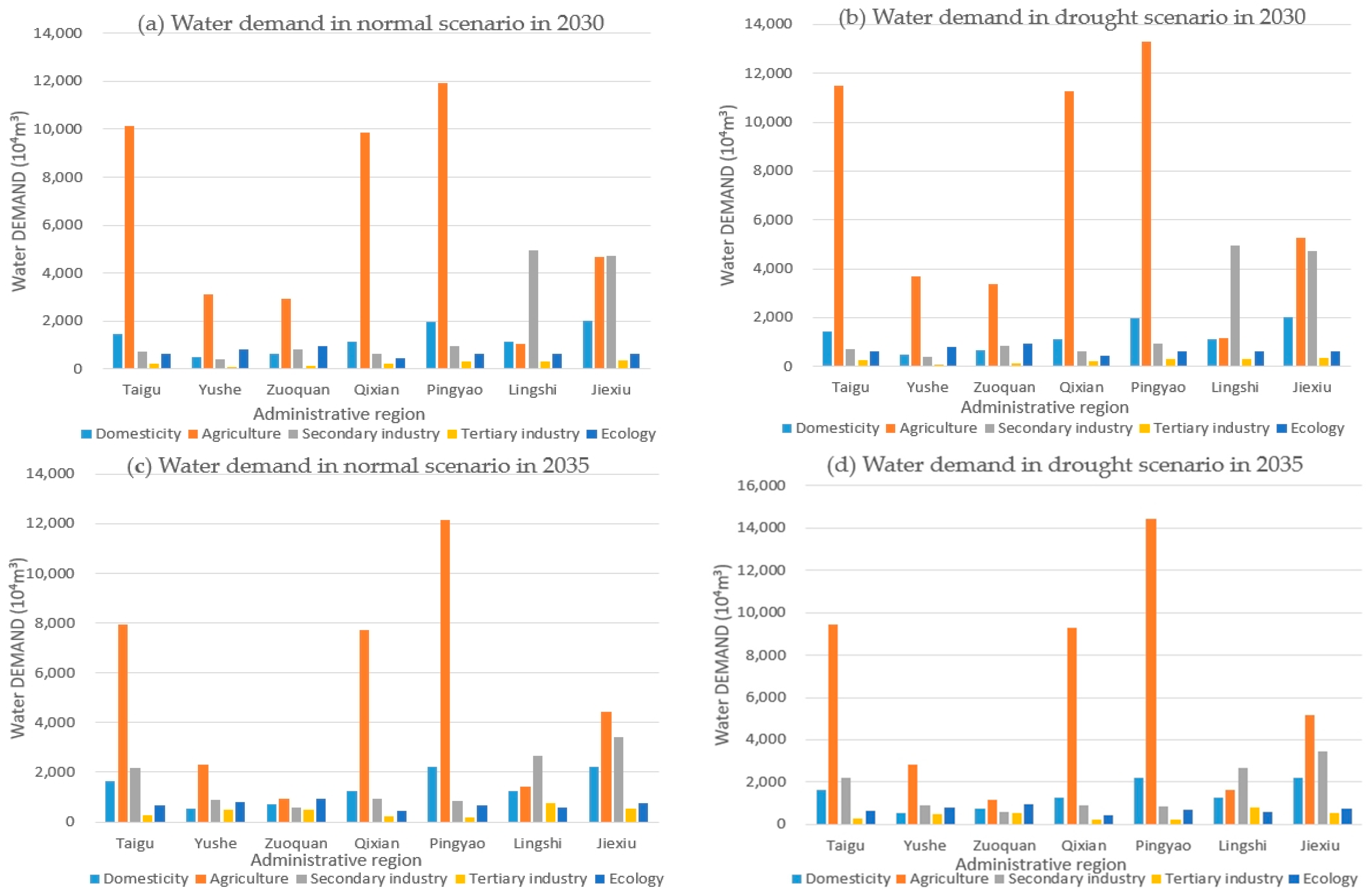
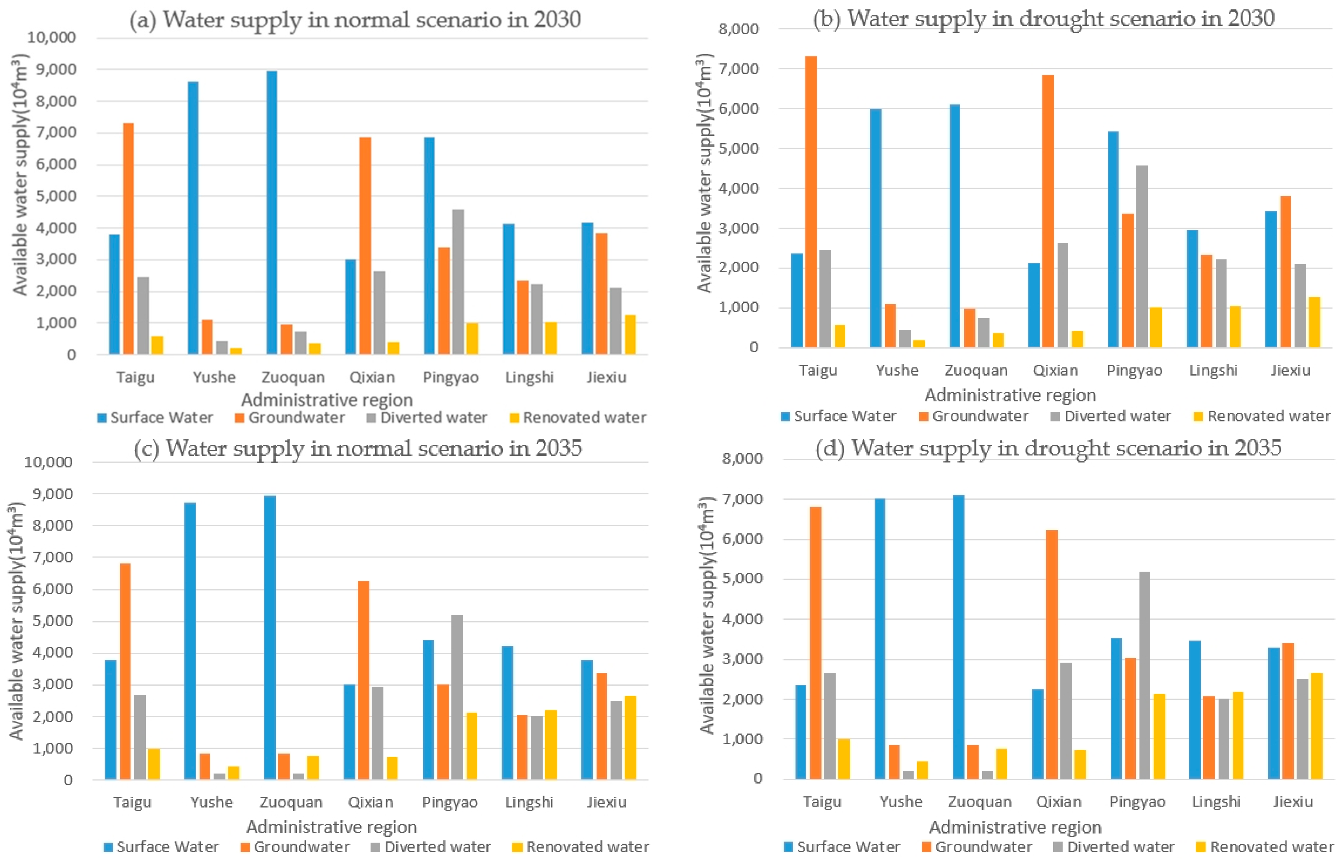
4.3. Water Supply and Demand Forecast

This study uses 2020 as the baseline year, with 2030 and 2035 as planning years, and selects normal (with a water inflow frequency of P = 50%) and drought scenarios (P = 75%) for the optimized allocation of water resources. Based on Jinzhong City’s future development plans, this study utilizes data from the Shanxi Province Water Resources Bulletin, Shanxi Province Water Use Quotas, Jinzhong City’s 2020 National Economic and Social Development Statistical Bulletin, and Jinzhong Statistical Yearbook to obtain information on current water use and economic and social development indicators. Using the quota method and trend analysis method, the water demand for each user in Jinzhong City during the planning level year is analyzed, and the Tennant method is used to calculate the ecological water demand within the river channels. The total water demand for 2030 in the normal and drought scenarios is calculated to be 71,903 × 10⁴ m³ and 77,796 × 10⁴ m³, respectively, while the total water demand for 2035 in the normal and drought scenarios is 66,196 × 10⁴ m³ and 73,282 × 10⁴ m³. The available water supply for different scenarios in the planning years for Jinzhong City is shown in Figure 3.

According to the Shanxi Water Conservation Action Plan Jinzhong Implementation Rules and the Jinzhong City Master Plan (2016–2030), by 2030 and 2035, the water supply sources in southern Jinzhong will include reclaimed water in addition to surface water, groundwater, and transferred water. Considering the uncertainty in the total available water supply and the varying water frequencies in different typical years, data from the 2006–2020 Jinzhong Statistical Yearbook and the Shanxi Province Water Resources Bulletin were used. Taking into account the current water supply capacity of existing hydraulic projects in the southern Jinzhong water supply area and the construction layout and progress of water diversion projects during the planning period, the projected available water supply for the planning years is shown in Figure 4. The amount of reclaimed water is calculated based on the water demand for residential living, tertiary industry, and industrial use in the planning years. The available water supply for the normal and drought scenarios in 2030 is 85,411 × 10⁴ m³ and 74,307 × 10⁴ m³, respectively, while in 2035, it is 87,202 × 10⁴ m³ and 77,915 × 10⁴ m³, respectively. Notably, with technological advancements, the available reclaimed water in 2035 is projected to be 9901 × 10⁴ m³, a significant increase from 4866 × 10⁴ m³ in 2030, effectively supplementing the local water resource gap.

4.4. Model Parameters

(1) Water Supply Benefit Coefficient $b_j^k$: By analyzing the relationship between the total output value of different industries in Jinzhong City and their water use quotas, and based on the DB14/T 1049.1-2020 Shanxi Province Water Use Quotas, the water supply benefit coefficients for the five categories of water users—domestic, agricultural, secondary industry, tertiary industry, and ecological—are calculated as follows: 600, 34.83, 638.30, 3413.60 CNY/m³, and 500 CNY/m³.

(2) Water Supply Cost Coefficient $c_j^k$: A detailed study of the 2020 water fee standards and supporting water price regulations in Jinzhong City determined the water supply cost coefficients for the five categories of water users—domestic, agricultural, secondary industry, tertiary industry, and ecological—as follows: 3.90, 0.25, 4.63, 5.80 CNY/m³, and 2.60 CNY/m³.

(3) Water Supply Priority Coefficient $a_i$: The water supply priority coefficient is determined by Formula (18):

$$a_i=(1+m_{max}-m_i)/\sum _{i=1}^I(1+m_{max}-m_i)$$

(18)

According to the water supply priority principle, the calculated water supply priority coefficients are as follows: surface water 0.4, groundwater 0.1, transferred water 0.3, and reclaimed water 0.2.

(4) Water Use Equity Coefficient ${\lambda }_j$: Based on the importance of various water users in Jinzhong City, the required water supply priority is in the following order: domestic water use, ecological water use, tertiary industry water use, secondary industry water use, and agricultural water use. Using Formula (18), the calculated water use equity coefficients are as follows: domestic water use 0.33, agricultural water use 0.07, secondary industry water use 0.13, tertiary industry water use 0.20, and ecological water use 0.27.

(5) Sewage Discharge Coefficient ${\alpha }_j^k$ and pollutant discharge concentration ${\beta }_j^k$: With reference to prior research [25], chemical oxygen demand (COD) was selected as the indicator for β in this study. The values of ${\alpha }_j^k$ and ${\beta }_j^k$ were determined based on China’s National Standard GB 50318-2017 Code for Urban Drainage Engineering Planning Standards [39] and, considering the actual sewage discharge situation in Jinzhong City, ecological water use is not included in the river pollution discharge calculation. Therefore, the COD concentration in the sewage discharged by domestic, agricultural, secondary industry, tertiary industry, and ecological water use for 2030 is set to 400, 200, 300, 500 mg/L, and 0 mg/L. The sewage discharge coefficient is set to 0.8, 0.2, 0.3, 0.8, 0.

(6) Minimum Water Supply Guarantee Rate ${\mathsf{\varepsilon }}_j^k$: Based on the actual water supply and demand situation in the study area and the water supply and demand forecast values for the planning year, the minimum water supply guarantee rates for domestic, agricultural, secondary industry, tertiary industry, and ecological water users in 2030 are set to 0.87, 0.7, 0.7, 0.80, and 0.80, respectively.

5. Results and Analysis

5.1. Evaluation of Scheme Effectiveness

Using MATLAB R2022b programming, the improved I-NSGA-III algorithm was employed to solve the water resource optimization allocation model for Jinzhong City. To identify the optimal parameters, data from the 2030 drought scenario were selected. Multiple crossover probabilities Pc and mutation probabilities Pm were configured to solve the developed water resources optimization allocation model. Each parameter combination was executed 20 times, and the Hypervolume (HV) indicator was used to evaluate the resulting Pareto front. Based on previous studies [30,40], commonly used crossover probabilities include Pc = 0.7, 0.8, and 0.9, while mutation probabilities are typically set as Pm = 0.05 or Pm = 1/D, where D denotes the number of decision variables in the model. The computational results are summarized in

Table 7. Computational Results of Hypervolume for Different Crossover and Mutation Probabilities in the 2030 Drought Scenario.

	Pm = 0.05		Pm = 1/D
	HV (Median)	HV (Std.)	HV (Median)	HV (Std.)
Pc = 0.7	0.42	2.56 × 10−5	0.48	3.15 × 10−5
Pc = 0.8	0.46	4.32 × 10−5	0.54	1.76 × 10−5
Pc = 0.9	0.37	6.32 × 10−5	0.45	1.58 × 10−5

. Ultimately, the crossover probability was set to Pc = 0.8, and the mutation probability was set to Pm = 1/D.

Relevant data were input, and the algorithm parameters were set as follows: population size N = 200, maximum number of iterations t_max = 200, crossover probability P_c = 0.8, mutation probability P_m = 1/D (where D is the number of decision variables in the model). The algorithm solves the model to obtain a Pareto set containing multiple solutions, which must be filtered to obtain a suitable configuration scheme. Here, TOPSIS is used to select the relatively optimal solution from the set of options. For the model’s three objective functions, no special adjustments are made, and their weights are considered equal, each being 1/3. In practical applications, decision-makers can set different objective weights based on personal preferences or use other evaluation methods to obtain a suitable water resource allocation scheme according to specific needs. The results of the water resource allocation for the planning year obtained using TOPSIS are shown in Figure 5.

The scheme with the highest comprehensive benefits was evaluated using a multi-system coupling coordination degree evaluation model (Section 3.2). The weights of the secondary indicators were calculated using the AHP method and the entropy weight method, with the weights of each indicator presented in Table 1. The coupling coordination degree of water resource allocation was obtained using Formulas (12)–(17), and the results are shown in

Table 8. Coupling coordination degree of different configuration schemes.

	Scheme	Economic Score	Social Score	Environmental Score	Comprehensive Score	Coupling Degree	Coordination Degree
2030	P = 50%	0.8512	0.4017	0.9967	0.7499	0.9315	0.8358
	P = 75%	0.6855	0.4416	0.7710	0.6327	0.9731	0.7847
2035	P = 50%	0.7097	0.6295	0.8783	0.7392	0.9904	0.8556
	P = 75%	0.7317	0.6207	0.9556	0.7693	0.9841	0.8701

.

According to the calculation results, after applying the I-NSGA-III algorithm, the coordination degree for Jinzhong City in 2030 under the normal scenario (P = 50%) is 0.8358, which indicates a good level of coordination. Under the drought scenario (P = 75%), the coordination degree is 0.7847, falling into the medium coordination level. In comparison, by 2035, the coordination degree under the normal scenario improves from 0.8358 to 0.8556 (an increase of 0.0199) and, under the drought scenario, it rises from 0.7847 to 0.8701 (an increase of 0.0855), both reaching a good coordination level. Combined with the water supply forecast results, it is evident that the extensive use of reclaimed water can improve regional coordination. However, the four optimized water resource allocation schemes still do not reach the optimal coordination threshold, indicating that solely relying on water resource allocation is insufficient to achieve system optimization; other regulatory measures are needed. Further analysis of system scores reveals that the economic system scores lower than the social and ecological systems, and the coordination degree is constrained by the balanced development of all systems. It is recommended to take measures to promote local economic development and improve the economic system’s score to further enhance coordination.

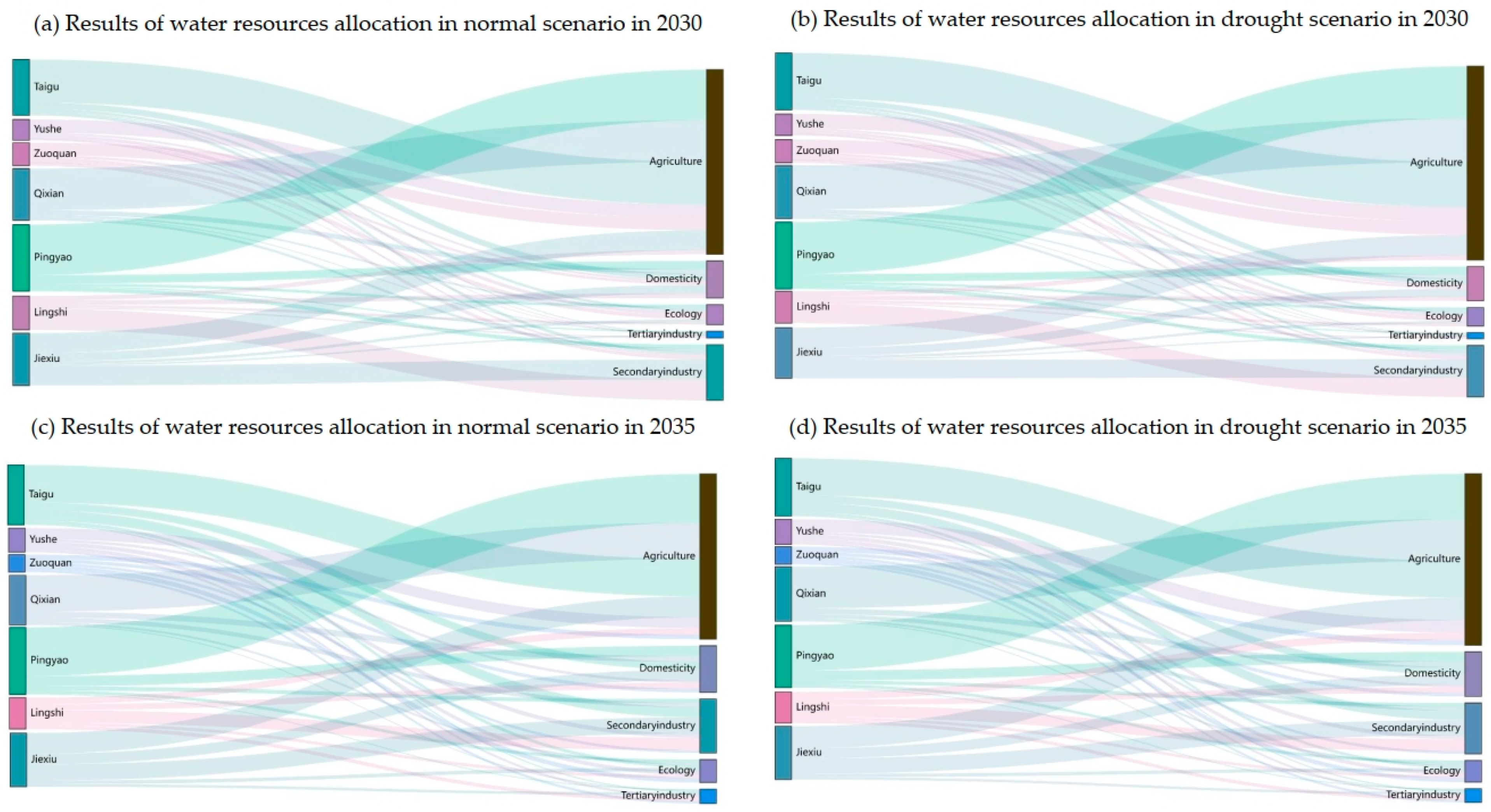
5.2. Water Resource Allocation Results

The specific values for each allocation scheme selected through the TOPSIS method are presented in

Table 9. Water resources allocation results of two schemes in 2030.

Scheme	Administrative Region	Domesticity	Agriculture	Secondary Industry	Tertiary Industry	Ecology	Total
Normal Scenario	Taigu	1454	10,139	731	237	633	13,194
	Yushe	490	3108	407	79	823	4907
	Zuoquan	644	2920	834	107	950	5455
	Qixian	1115	9857	610	207	435	12,224
	Pingyao	1965	11,939	934	289	624	15,751
	Lingshi	1115	1023	4939	325	614	8016
	Jiexiu	1998	4134	4329	329	576	10,966
	Total	8781	43,120	12,784	1573	4655	70,913
Drought Scenario	Taigu	1375	9894	660	208	596	12,733
	Yushe	490	3666	407	79	823	5465
	Zuoquan	644	3384	834	107	950	5919
	Qixian	1015	9878	560	175	405	12,033
	Pingyao	1837	10,883	874	236	573	14,403
	Lingshi	1115	1172	4939	325	614	8165
	Jiexiu	1758	3903	4115	294	563	10,632
	Total	8232	42,780	12,388	1424	4525	69,349

(Unit: 10⁴ m³).

and

Table 10. Water resources allocation results of two schemes in 2035.

Scheme	Administrative Region	Domesticity	Agriculture	Secondary Industry	Tertiary Industry	Ecology	Total
Baseline Scenario	Taigu	1644	7927	2177	287	662	12,697
	Yushe	551	2322	890	503	818	5084
	Zuoquan	720	944	580	514	955	3713
	Qixian	1244	7716	925	230	452	10,567
	Pingyao	2205	10,327	804	192	631	14,159
	Lingshi	1242	1404	2648	773	602	6669
	Jiexiu	2223	4425	3425	554	751	11,377
	Total	9828	35,064	11,450	3054	4871	64,268
Water—Saving Scenario	Taigu	1644	8203	2089	287	630	12,853
	Yushe	551	2832	890	503	818	5594
	Zuoquan	720	1141	580	514	955	3911
	Qixian	1244	9278	925	230	452	12,129
	Pingyao	2205	10,089	780	199	617	13,890
	Lingshi	1242	1652	2648	773	602	6917
	Jiexiu	2223	4926	3403	541	739	11,832
	Total	9828	38,121	11,316	3048	4813	67,127

(Unit: 10⁴ m³).

. The allocation results comply with the Comprehensive Wastewater Discharge Standard of Shanxi Province (DB14/1928–2019) [41].

(1) Analysis of Water Allocation by Sector. The distribution ratios of water allocation for various users under different scenarios in the planning year are shown in Figure 6. As depicted, agricultural water use in Jinzhong City is the highest, accounting for 54% to 62%. With the promotion of water-saving technologies and adjustments in planting structures, the demand for agricultural water in 2035 is 5% to 7% lower than in 2030. Industrial water use ranks second, comprising 17% to 18% of the total. This is followed by residential and ecological water use. Notably, the proportion of water use by tertiary industry increases from 2% to 4% or 5% by 2035. Due to population growth and the advancement of urbanization, people’s needs have shifted, leading to significant development in the service industry and related sectors, thereby increasing water demand accordingly.

(2) Analysis of Configuration Objectives. An analysis of the objective values for the optimized water resource allocation scheme in Jinzhong City is presented, with the benefit values of the three objective functions for different allocation schemes shown in

Table 11. The target values of different planning schemes.

	Scheme	Water Shortage (104 m3)	Economic Benefit (108 CNY)	COD Emission (104 t)
2030	P = 50%	1390	175.6215	6.3144
	P = 75%	8447	161.9397	6.0303
2035	P = 50%	1319	218.1919	6.7996
	P = 75%	6155	212.7355	6.9074

. The results indicate that, in the planning year 2030, as the water frequency increases, the social benefit objective function also increases, with the water shortage rising to 84.47 million m³, indicating a severe water scarcity situation. With the increase in water frequency, the economic benefit objective decreases from 17.56215 billion CNY to 16.19397 billion CNY, and the total COD emissions in wastewater also decrease from 63,144 tons to 60,303 tons. This phenomenon reveals the characteristics of multi-objective optimization problems, where different objective functions influence each other and often have conflicting relationships; an improvement in one objective’s benefit often leads to a decline in others. Comparing the planning years 2035 and 2030, the water shortage decreases and economic benefits increase, but pollutant emissions also rise. This is because the available reclaimed water supply in 2035 further increases compared to 2030, optimizing the water supply structure. With technological upgrades and industrial structure optimization, the demand for water use in the high-benefit tertiary industry increases, generating more economic benefits but also more pollutants.

6. Discussion

(1) Jinzhong City is a typical resource-scarce city with diverse industries and developed agriculture. The insufficiency of surface water resources has led to the over-extraction of groundwater, forming a funnel area that severely impacts local ecological health and sustainable development. To alleviate the conflict between water supply and demand, a multi-objective water resource optimization model is established, comprehensively considering social, economic, and ecological benefits. Previous studies on Jinzhong City have only considered two objectives in water resource allocation models [42], which are relatively simple. In contrast, this study uses three objective functions: minimizing water shortages, maximizing economic benefits, and minimizing emissions of major pollutants. The model is constrained by water supply balance, supply capacity, total water usage, and non-negativity of variables, providing a more comprehensive approach to optimizing water resource allocation. Since the data used in this model is specific and can be adjusted for different regions, it can be applied to other similar water-scarce cities.

(2) A comparative analysis of the water demand data for the current and planning years in Jinzhong City reveals an increase in water supply for the planning years, with the available water supply in 2035 exceeding that of 2030. This is due to the further increase in reclaimed water supply in 2035, which improves the regional water supply structure and effectively alleviates the tension of insufficient water resources. This aligns with existing policy documents such as the 14th Five-Year Plan of Shanxi Province and the Jinzhong City Central Urban Area Water Supply Special Plan (2024ZXG-036). In the current year, the production of reclaimed water is relatively low, and its price is similar to that of regular water, leading to low acceptance and utilization by enterprises. Most reclaimed water is directly used to supplement river flows, with the excess beyond ecological needs resulting in waste. Therefore, managers need to provide specific guidance measures, such as reducing the price of reclaimed water and constructing comprehensive reclaimed water supply pipelines to lower the barriers to its use, thereby encouraging enterprises to recognize and use reclaimed water.

(3) In multi-objective optimization problems with constraints, the Pareto front is unknown and can vary due to the influence of these constraints. The reference points in the traditional NSGA-III algorithm are predefined, which may not accurately reflect the development trend of the Pareto front. To address this issue, this study improves the NSGA-III algorithm by incorporating a reference point adjustment strategy, a dynamic solution retention mechanism, and a selection strategy, resulting in the I-NSGA-III algorithm. Comparative experiments using test functions show that the IGD metric of I-NSGA-III is reduced by 5.17% to 50.22%, and the HV metric is increased by 2.47% to 7.63%, demonstrating that this algorithm offers better optimization accuracy and overall performance.

(4) A comparison of the allocation schemes across different planning years shows that, under the drought scenario, water shortages increase and economic benefits decline compared to the normal scenario. However, COD emissions decrease due to reduced water consumption, highlighting a significant trade-off between economic objectives and ecological and social goals. This result aligns with the “economic–ecological” conflict observed by Wu Yun et al. [7] in their study on water resource optimization in Shanxi Province. However, this study further quantifies the trade-off relationships between different objectives through the design of water-saving scenario. Additionally, the high proportion of agricultural water shortages is closely related to the high demand for agricultural water in Jinzhong City and its low supply priority. This phenomenon echoes the findings of Li Muhan et al. [36] in Yangquan City, underscoring the importance of optimizing the agricultural water use structure. It is recommended to adopt more scientific irrigation methods and promote water-saving renovations to improve irrigation water use efficiency and reduce agricultural water losses.

(5) Despite the contributions of this study, certain limitations remain. This research establishes a water resource optimization model and improves the algorithm specifically for water-scarce regions, with the primary goal of alleviating the regional water supply and demand conflict. In contrast, in regions with more abundant water resources, the aim of water resource optimization is typically to achieve high-quality development. Therefore, different water conditions and objectives pose challenges to the improved algorithm presented in this study. In the future, we will collect data from corresponding regions to conduct water resource optimization studies to validate the algorithm’s performance. Additionally, the water demand forecasting in this study relies on current water usage data. In future research, we will employ other forecasting methods: 1. Introducing socio-economic scenario analysis: Designing multiple scenarios based on Shared Socio-economic Pathways (SSPs), such as high growth-high water consumption and low carbon-water-saving societies, to quantify water demand under different development paths. 2. Using uncertainty modeling methods, such as Stochastic Programming: Treating climate change and socio-economic variables as random parameters to construct a two-stage optimization model.

(6) Our current research focuses on improving the effectiveness of the algorithm and the quality of the solutions, without analyzing the potential increase in computational overhead introduced by the improved algorithm. In future research, we can evaluate computational overhead by comparing the average runtime per generation for DTLZ series problems. Additionally, we can explore adaptive triggering mechanisms—activating reference point updates only when population diversity falls below a certain threshold—to balance solution quality with computational efficiency.

7. Conclusions

This study addresses the water supply–demand conflict in Jinzhong City by establishing a multi-objective optimization model encompassing economic, social, and ecological objectives. An improved I-NSGA-III algorithm is proposed, integrating adaptive reference point generation, dynamic solution retention mechanisms, and optimized selection strategies to enhance algorithmic performance and achieve scientifically sound regional water resource allocation. The main conclusions are as follows:

(1) The I-NSGA-III algorithm overcomes the limitations of NSGA-III’s predefined fixed reference points by dynamically adjusting reference point distributions. Combined with an early-stage high-quality solution retention strategy, it significantly improves solution set convergence and diversity. Experimental results demonstrate reductions of 5.17–50.22% in the IGD metric and increases of 2.71–25.51% in the HV metric across the DTLZ test functions, validating its effectiveness for complex constrained multi-objective optimization problems.

(2) The coupled coordination degree evaluation model innovatively incorporates system synergy theory into water resource allocation assessment, quantifying interactions among economic, social, and ecological objectives. Results show coordination degrees of 0.8556–0.8701 for 2035 scenarios (compared to 0.7847–0.8358 in 2030), confirming that the optimized schemes effectively mitigate multi-system conflicts in Jinzhong City.

(3) Through increased reclaimed water utilization (reaching 9901 × 10⁴ m³ in 2035, a 103.6% increase from 2030) and optimized water supply structures, economic benefits under the 2035 P = 50% scenario rise by 42.57 × 10⁸ CNY compared to baseline levels. Meanwhile, COD emissions remain controlled at 6.03 × 10⁴–6.91 × 10⁴ tons, demonstrating the model’s practical value in balancing multi-objective conflicts.

References

1. Abdulbaki, D.; Al-Hindi, M.; Yassine, A.; Yassine, A.; Abou Najm, M. An optimization model for the allocation water resources. J. Clean. Prod. 2017, 164, 994–1006. [Google Scholar] [CrossRef]
2. Zhang, F.; Wu, Z.; Di, D.; Wang, H. Water resources allocation based on water resources supply-demand forecast and comprehensive values of water resources. J. Hydrol. Reg. Stud. 2023, 47, 101421. [Google Scholar] [CrossRef]
3. Wei, F.; Zhang, X.; Xu, J.; Bing, J.; Pan, J.G. Simulation of water resource allocation for sustainable urban development: An integrated optimization approach. J. Clean. Prod. 2020, 273, 122537. [Google Scholar] [CrossRef]
4. Genova, P.; Wei, Y. A socio-hydrological model for assessing water resource allocation and water environmental regulations in the Maipo River basin. J. Hydrol. 2023, 617, 129159. [Google Scholar] [CrossRef]
5. Liu, W. Analysis of urban water resources pollution control and environmental protection. Heilongjiang Environ. J. 2025, 38, 118–120. [Google Scholar]
6. Jia, Z.; Liu, P.; Ma, Y.; Zheng, F. An Analysis of the Dynamic Evolution and Utilization of Water Resources in China. Water Resour. Power 2023, 41, 27–30. [Google Scholar] [CrossRef]
7. Wu, Y.; Zeng, C.; Yang, K.; Yu, Y.; He, Q.; Zhong, X. Multi-objective optimal allocation of water resources based on improved NSGA-II algorithm. Yellow River 2020, 42, 71–75. [Google Scholar]
8. Yuan, Z.; Yang, K.; Chen, J.; Qian, L.; Li, Z.; Wu, J. Multi-objective optimal allocation scheme decision of regional water resources based on NSGA-III. Yellow River 2024, 46, 79–84+153. [Google Scholar]
9. Haimes, Y.Y.; Lasdon, L.S.; Wismer, D.A. On a Bicriterion Formulation of the Problems of Integrated System Identification and System Optimization. In IEEE Transactions on Systems, Man, and Cybernetics; IEEE Advancing Technology for Humanity: Piscataway, NJ, USA, 1971; Volume SMC-1, pp. 296–297. [Google Scholar] [CrossRef]
10. Haimes, Y.Y.; Hall, W.A. Multiobjectives in water resource systems analysis: The Surrogate Worth Trade Off Method. Water Resour. Res. 1974, 10, 615–624. [Google Scholar] [CrossRef]
11. Loucks, D.P.; van Beek, E. (Eds.) Modeling Uncertainty. In Water Resource Systems Planning and Management: An Introduction to Methods, Models, and Applications; Springer International Publishing: Cham, Switzerland, 2017; pp. 301–330. [Google Scholar]
12. Roozbahani, R.; Schreider, S.; Abbasi, B. Economic sharing of basin water resources between competing stakeholders. Water Resour. Manag. 2013, 27, 2965–2988. [Google Scholar] [CrossRef]
13. Choi, B.; Lee, G.; Lee, M. Modeling and stochastic dynamic optimization for optimal energy resource allocation. Comput. Aided Chem. Eng. 2012, 31, 765–31769. [Google Scholar]
14. Holland, J.H. Genetic algorithms. Sci. Am. 1992, 267, 66–73. Available online: https://www.jstor.org/stable/24939139 (accessed on 15 November 2024). [CrossRef]
15. Arabi, M.; Govindaraju, R.S.; Hantush, M.M. Cost-effective allocation of watershed management practices using a genetic algorithm. Water Resour. Res. 2006, 42, 2405–2411. [Google Scholar] [CrossRef]
16. Kennedy, J.; Eberhart, R.C. Particle swarm optimization. In Proceedings of the ICNN’95-International Conference on Neural Networks, Perth, WA, Australia, 27 November–1 December 1995. [Google Scholar]
17. Jahandideh-Tehrani, M.; Bozorg-Haddad, O.; Loáiciga, H.A. Application of particle swarm optimization to water management: An introduction and overview. Environ. Monit. Assess. 2020, 192, 281. [Google Scholar] [CrossRef] [PubMed]
18. Kirkpatrick, S.; Gelatt, J.C.D.; Vecchi, M.P. Optimization by simulated annealing. Science 1983, 220, 671–680. [Google Scholar] [CrossRef]
19. Aerts, J.C.J.H.; Heuvelink, G.B.M. Using simulated annealing for resource allocation. Int. J. Geogr. Inf. Sci. 2002, 16, 571–587. [Google Scholar] [CrossRef]
20. Zhang, J.; Dong, Z.; Chen, T. Multi-Objective Optimal Allocation of Water Resources Based on the NSGA-2 Algorithm While Considering Intergenerational Equity: A Case Study of the Middle and Upper Reaches of Huaihe River Basin, China. Int. J. Environ. Res. Public Health 2020, 17, 9289. [Google Scholar] [CrossRef]
21. Baltar, A.M.; Fontane, D.G. Use of multiobjective particle swarm optimization in water resources management. J. Water Resour. Plan. Manag. 2008, 134, 257–265. [Google Scholar] [CrossRef]
22. Zhang, Q.; Li, H. MOEA/D: A Multiobjective Evolutionary Algorithm Based on Decomposition. In IEEE Transactions on Evolutionary Computation; IEEE Computational Intelligence Society: Park Avenue, NY, USA, 2007; Volume 11, pp. 712–731. [Google Scholar] [CrossRef]
23. Liu, X.; Zhao, X.; Wu, W.; Yao, L.; Guo, Q. Optimal allocation of water resources in Taiyuan City based on NSGA-II + ARSBX algorithm. Adv. Sci. Technol. Water Resour. 2025, 45, 79–86+103. [Google Scholar]
24. Li, Z.; Zhao, X.; Li, J.; Li, Y. Research on the optimal allocation of water resources in Yangquan City based on improved particle swarm optimization algorithm. J. N. China Univ. Water Resour. Electr. Power 2024, 45, 15–21. [Google Scholar]
25. Li, C.; Jiang, H.; He, Y.; Mu, Z. Study on water resources allocation and scheme optimization based on WRMM model. J. Water Resour. Water Eng. 2016, 27, 32–38. [Google Scholar]
26. Bezdan, A.; Bezdan, J.; Marković, M.; Mirčetić, D.; Baumgertel, A.; Salvai, A.; Blagojević, B. An objective methodology for waterlogging risk assessment based on the entropy weighting method and machine learning. CATENA 2025, 249, 108618. [Google Scholar] [CrossRef]
27. Guo, J.; Jiang, Z.; Ying, J.; Feng, X.; Zheng, F. Optimal allocation model of port emergency resources based on the improved multi-objective particle swarm algorithm and TOPSIS method. Mar. Pollut. Bull. 2024, 209, 117214. [Google Scholar] [CrossRef]
28. Yuan, L.; Liu, H.; Lu, Y.; Zhou, C.; Zhou, C.; Lu, Y. Multi-objective integrated decision method of cascade hydropower stations based on optimization algorithm and evaluation model. J. Hydrol. 2024, 638, 131533. [Google Scholar] [CrossRef]
29. Zhao, Q.; Bai, Q.; Nie, K.; Wang, H.; Zeng, X. Multi-objective optimal allocation of regional water resources based on NSGA-III algorithm and TOPSIS decision. J. Drain. Irrig. Mach. Eng. 2022, 40, 1233–1240. [Google Scholar]
30. Deb, K.; Jain, H. An evolutionary many-objective optimization algorithm using reference-point-based nondominated sorting approach, part I: Solving problems with box constraints. IEEE Trans. Evol. Comput. 2014, 18, 577–601. [Google Scholar] [CrossRef]
31. Jain, H.; Deb, K. An evolutionary many-objective optimization algorithm using reference-point based nondominated sorting approach, part II: Handling constraints and extending to an adaptive approach. IEEE Trans. Evol. Comput. 2014, 18, 602–622. [Google Scholar] [CrossRef]
32. Das, I.; Dennis, J.E. Normal-boundary intersection: A new method for generating the Pareto surface in nonlinear multicriteria optimization problems. SIAM J. Optim. 1998, 8, 631–657. [Google Scholar] [CrossRef]
33. Bi, X.; Wang, C. An improved NSGA-III algorithm based on objective space decomposition for many-objective optimization. Soft Comput. 2017, 21, 4269–4296. [Google Scholar] [CrossRef]
34. Yuan, T.; Yin, Y.; Huang, F.; Chen, Y. Adaptive weight adjustment MOEA/D with global replacement. Control. Theory Appl. Control. Theory Appl. 2023, 40, 653–662. [Google Scholar]
35. Changming, J.; Haoyu, M.; Yang, P. Research on evolutionary algorithm for multi-objective optimal operation of cascade reservoirs. J. Hydraul. Eng. 2020, 51, 1441–1452. [Google Scholar]
36. Jia, Z.; Zhao, X.; Cui, C. Research on decision-making method of water resources allocation based on coordinated equilibrium. Henan Water Resour. South–North Water Divers. 2020, 49, 35–37. [Google Scholar]
37. Fu, L.; Yang, K.; Liu, J.; Zhong, J.; Qiu, G.; Gu, G.; Jiang, M.; Wang, X.; Liang, Y. Evaluation model of reclaimed water based on multi-level superiority evaluation method. Water Resour. Power 2018, 36, 34–37. [Google Scholar] [CrossRef]
38. Wang, Q.; Zhao, S. Research on the spatial-temporal coupling coordination of carbon emission-technological innovation-green development in the Yangtze River Economic Belt. Resour. Environ. Yangtze Basin 2025, 34, 494–506. [Google Scholar]
39. GB 50318-2017; Code for Planning of Urban Drainage Engineering. Ministry of Housing and Urban-Rural Development of the People’s Republic of China: Beijing, China, 2017.
40. Li, M.; Zhao, X.; Zhang, Z.; Zuo, Q. An optimal allocation model of water resources in water-deficient areas for high-quality development and its application. Yellow River 2024, 46, 73–79. [Google Scholar]
41. DB14/1928-2019; Integrated Wastewater Discharge Standards. Shanxi Provincial Department of Ecology and Environment: Taiyuan, China, 2019.
42. Zhu, S.; Li, Z. Optimal allocation of water resources in Jinzhong City based on improved NSGA-II algorithm. China Rural. Water Hydropower 2023, 91–97+105. Available online: https://link.cnki.net/urlid/42.1419.TV.20220711.1416.079 (accessed on 23 May 2025).
Figure 1. Comparison of Pareto Fronts for DTLZ1-4.
Applsci 15 05963 g001
Figure 2. Network diagram of water supply system.
Applsci 15 05963 g002
Figure 3. Water demand for each administrative region in planning year.
Applsci 15 05963 g003
Figure 4. Water supply of each administrative region in the planning year.
Applsci 15 05963 g004
Figure 5. Water resources allocation results for each administrative region in planning year.
Applsci 15 05963 g005
Figure 6. The proportion of water consumption in different scenarios of each water user in the planning year.
Applsci 15 05963 g006aApplsci 15 05963 g006b