Artificial Intelligence-Based Models for Estimating and Extrapolating Soiling Effects on Photovoltaic Systems in Spain

Abstract

Environmental and temporal conditions, particularly dust accumulation, can significantly impact the performance of photovoltaic solar panels, potentially reducing their efficiency by up to 20%, and thereby affecting profitability. Accurately estimating these losses is crucial for optimising maintenance and avoiding unforeseen losses. Various models have been proposed in the literature for this purpose. In this context, four machine learning models were developed using meteorological and air quality data from the Solar Energy Research Center (CIESOL). A Gradient-Boosting model (LightGBM) and a neural network achieved RMSE values of 0.68% and 0.88% of soiling loss, and $R^2$ values of 0.86 and 0.76 between measured and estimated values, respectively, on their test sets. The generalisation capability of these models was tested by extrapolating them to other regions in Spain. To enhance robustness across locations, a global artificial neural network (ANN) model was trained using combined data from two sites, achieving an RMSE of 1.02% when estimating soiling losses. This result highlights a significant improvement over models trained on a single location and tested elsewhere, demonstrating the global model’s stronger ability to generalise across different geographic settings.

1. Introduction

Photovoltaic solar energy systems represent a reliable and efficient source of electricity generation. Globally, photovoltaic solar energy accounts for 13% of the total installed capacity for electricity production, generating 4% of the world’s electricity. By 2050, photovoltaic solar energy is expected to constitute 49% of the installed power if current policies continue. In this way, photovoltaic solar energy would increase from 31% of the installed renewable capacity to 66%, making it the renewable energy source with the most significant growth among the main sources [1]. Alongside this expansion, wind power continues to play a complementary role, with the global installed capacity surpassing 1170 GW in 2024, led by strong deployment in China [2]. Meanwhile, green hydrogen is emerging as a key solution for storing excess renewable energy and decarbonizing hard-to-electrify sectors. Although hydrogen is currently the most expensive form of hydrogen, compared to gray and blue hydrogen, recent techno-economic studies suggest that green hydrogen can benefit from declining renewable electricity costs, improvements in electrolyser efficiency, and government incentives. These factors are expected to reduce costs over time, supporting the broader integration of photovoltaic solar energy and other renewable sources into the energy system [3].

However, multiple environmental and physical factors significantly affect the performance of photovoltaic solar panels [4]. Elevated operating temperatures, for instance, can reduce panel efficiency by approximately 0.52% per degree Celsius increase in operating temperature, with a total efficiency drop of 27.4% when the temperature rises from 25 °C to 75 °C [5]. In addition, working with suboptimal tilt angles can reduce the efficiency of photovoltaic panels. According to a numerical and experimental investigation by Mamun et al. [6], for every 5° increments in the angle of surface tilt, efficiency falls by 0.35% and 0.33% for experimental and numerical cases, respectively. Ageing is also an important factor. A study conducted in Baghdad, Iraq, observed that monocrystalline photovoltaic modules exhibited a degradation rate of approximately 0.593% per year over an eight-year period, leading to a total performance loss of approximately 4.74% [7].

One of the most important factors in the production of solar photovoltaic plants is the presence of dust. The presence of suspended particles in the atmosphere precipitates on the earth’s surface, taking into account environmental factors such as wind or relative humidity, among other physical factors. These particles, once settled on the solar panel, cause a reduction in the effective solar irradiance of the solar cells, thus decreasing the performance of the panel due to natural causes. This effect can decrease the performance of a PV plant by almost 20%, thus reducing the profitability of the installation [8]. In a 50 MWp plant, these losses can account for a monthly reduction in production of up to 500 MWh with annual losses of more than EUR $\mathrm{220,000}$ [9]. Mitigating these effects can also lead to a reduction in benefits, as it increases operational costs and the capital invested. This is especially notable in regions with arid and semi-arid climates, such as desert areas, where solar radiation levels are particularly high and airborne dust is highly intrusive [10].

The role of meteorological variables in the influence of soil loss is crucial. For example, humidity has a negative impact on the power output of photovoltaic panels, turning dust into mud as it increases [11]. It can also alter the irradiance non-linearly and irradiance itself causes large variations in short-circuit current linearity, affecting efficiency [12]. Meanwhile, the wind speed can influence both the dust deposition and the cooling of the panels, leading to positive or negative effects depending on the speed and direction of the wind [13].

The maintenance of the performance of solar panels has been closely linked to strategies for managing soils, with preventive and cleaning methods playing a significant role. Various approaches for anti-dust coatings have been studied and tested as preventive measures [14,15,16]. Khan et al. (2024) experimented with various configurations of anti-dust coatings and tracking systems in the desert region of Saudi Arabia, achieving a reduction in soiling losses of up to 85 % by combining anti-soil coatings with tracking that includes vertical night stowage [17].

There are different models in the literature that are used to estimate soiling losses, including both physical–statistical models and artificial intelligence models. Examples include an exponential model correlating dust deposition density with power losses [18] and an optical model that calculates dust deposition based on particulate mass concentration, precipitation, and other variables [19], and thereby determines the loss of light transmittance [20]. In the field of machine learning, the most widely used models are artificial neural networks. Among the main disadvantages of current models are their high dependence on the location where the data for the model were obtained and their inflexibility when changing the design region [21].

In this context, given the importance of modelling soiling losses in photovoltaic panels, in this work, we have developed various machine learning models tailored for this purpose. The focus has been on easily accessible meteorological variables, such as atmospheric temperature, wind speed, relative humidity, particulate matter (PM_2.5, PM₁₀), and others, which are continuously monitored worldwide and available from satellites. These models aim to create reliable estimations and can be extrapolated to different locations. Specifically, models were initially developed and tested for the location of Almería, Spain, and then evaluated for their ability to extrapolate to another location: Madrid, Spain. In particular, a global model was trained using combined data from both locations and demonstrated strong generalizability, achieving a root mean square error (RMSE) of 1.02% in predicting soil erosion losses. This result underscores the effectiveness and applicability of the approach in varying geographic and climatic conditions.

This article is organised into several sections. The Materials and Methods Section details the data acquisition process, including the sources and types of meteorological data used, as well as the data processing techniques applied to prepare the data for analysis. It also describes the development of four different machine learning approaches used to predict soiling losses in photovoltaic panels. The results present the outcomes of these models, evaluating their performance in the initial location (Almería), their extrapolation to a different location (Madrid), and the development and results of a global model trained on data from both locations. The Conclusions Section summarises the key findings of the study, emphasising the effectiveness and limitations of the developed models.

2. Materials and Methods

2.1. Photovoltaic System CIESOL

The experimental setup is located on the roof of the Solar Energy Research Centre (CIESOL) at the University of Almería (Spain) (${36.83}^{\circ }$ N, ${2.40}^{\circ }$ W, at sea level). It consists of two south-oriented silicon polycrystalline photovoltaic panels, ATERSA A222-P, whose electrical characteristics are displayed in

Table 1. Electrical characteristics of the Atersa A222P photovoltaic panel.

Parameter	Value
Maximum Power ($P_{\max }$)	222 W
Efficiency ($\eta$)	$13.63\%$
Short-circuit Current ($I_{\mathrm{SC}}$)	8.17 A
Open-circuit Voltage ($V_{\mathrm{OC}}$)	36.42 V

, with the same angle of inclination (${22}^{\circ }$) as a nearby photovoltaic plant with a power of $9.32\mathrm{kWp}$. For data collection, it was necessary to maintain the western one regularly, while the eastern one was kept maintenance-free (see Figure 1) to measure the difference in the short-circuit current between them both based on the shunt resistance. This difference is attributed to the accumulation of dust on the western panel, which reduces its short-circuit current output.

There is also a weather station on the roof of CIESOL where several environmental variables are monitored, such as particulate matter, irradiance, relative humidity, temperature, and precipitation, among others.

2.2. Data Processing

In

Table 2. Variables monitored by sensors in the CIESOL station.

Measure	Sensor	Unit	$\Delta$ Measure
Short Circuit Current	KAINOS Shunt KL.0.5 15 A/150 mV	A	$\pm 1\times {10}^{-2}$ A
Ambient Temperature	Biral SWS-250	°C	$\pm 5\%$
PM2.5	Aeroqual AQS1	μg/m3	±1 × 10−1 μg/m3
PM10	Aeroqual AQS1	μg/m3	±1 × 10−1 μg/m3
Relative Humidity	Vaisala HMP60	%	$\pm 3\%$
Wind speed	WMO-Station ID 08487	km/h	$\pm 0.1$ km/h
Precipitation	Biral SWS-250	mm	$\pm 3\times {10}^{-4}$ mm

the different variables that have been monitored in both the experimental setup and the weather station are displayed. Since there were data gaps during most of the time series for wind speed, the data for this variable were obtained from a weather station at the Airport of Almería (${36.85}^{\circ }$ N, ${2.38}^{\circ }$ W), whose identification number at the World Meteorological Organisation (WMO) is 08487.

These sensors provided a value for each measure every minute from 2 February 2024 to 31 May 2024 with two periods during which some data were missing. The first period extended from 31 July 2023 to 21 September 2023, and the second from 11 February 2024 to 23 March 2024. The night data were eliminated using the zenith angle that drops below ${90}^{\circ }$ during the day. Since soiling data are best measured at central times of the day and to remove some erroneous data caused by shadowing, all data points corresponding to a zenith angle over ${75}^{\circ }$ in the morning and over ${65}^{\circ }$ in the afternoon were excluded. This filtering process resulted in a dataset of 176,518 one-minute data instances. To calculate Soiling Loss (SL) as a percentage, Equation (1) was used [22]. Calibration was performed to ensure that any difference between the measurements of the two panels was attributable solely to soiling.

$$SL[\%]=100·{\displaystyle \frac{\frac{I_{sc,\mathrm{maintained}\mathrm{panel}}}{I_{sc,\mathrm{maintained}\mathrm{panel},\mathrm{ref}}}-\frac{I_{sc,\text{maintenance-free}\mathrm{panel}}}{I_{sc,\text{maintenance-free}\mathrm{panel},\mathrm{ref}}}}{\frac{I_{sc,\mathrm{maintained}\mathrm{panel}}}{I_{sc,\mathrm{maintained}\mathrm{panel},\mathrm{ref}}}}}$$

(1)

In addition, a computed variable called days without rain or days since last rain (DSLR) was calculated. This variable measures how many days have passed since it rained enough to clean solar panels and reduce soiling losses. The chosen threshold for rain accumulation to trigger cleaning is crucial: too low a threshold may result in incomplete cleaning, while too high a threshold might delay resetting the variable. Coello and Boyle [19] used a 1 mm threshold in their simple model and observed that when the threshold is lower than that, e.g., 0.5 mm, the model experiences more frequent cleaning events. In an experiment in Jaén, Spain, [23] different cleaning thresholds (CTs) were tested in some existing models, and the best results were obtained for a CT of 0.3 mm/day.

The CT that adjusted best to the soiling loss measured in Almería, Spain, in this experiment was 0.1 mm/day, as seen in Figure 2, which shows how three different CTs affect the computed variable DSLR and how these different DSLR computations fit the soiling losses calculated earlier.

As can be seen in Figure 2, the measured soiling values vary throughout the year. The absence of rainfall is indicative of a constant increase over time, although the periods with the highest dust presence in the photovoltaic panels usually correspond to the spring months, when losses of around 15% are reached. Therefore, the number of days without rain, together with the amount of rainfall, is a very decisive factor in interpreting the cleanliness factor achieved. The testing facility is located at sea level, so, no influence of industry or contaminant processes can be considered to contribute to the presence of dust on the PV panels.

Another variable was calculated: PM_10–2.5, consisting of the concentration of particulate matter for particles whose diameter is greater than 2.5 μm and smaller than 10 μm. Equation (2) was used to calculate this. This calculation was performed to avoid overlap, since $P{M}_{10}$ considers all forms of particulate matter whose diameter is less than 10 μm, which includes $P{M}_{2.5}$ (a diameter of less than 2.5 μm).

$$P{M}_{10-2.5}=P{M}_{10}-P{M}_{2.5}$$

(2)

The data were transformed from minute-long intervals to daily intervals, resulting in a total of 322 days for the variables shown in

Table 3. Variables used to develop the models.

Variable	Unit
Soiling Loss (SL)	%
Ambient temperature	°C
PM2.5	μg/m3
PM10–2.5	μg/m3
Relative Humidity (RH)	%
Wind Speed (Wspeed)	km/h
Precipitation	mm/days
Days since last rainfall (DSLR)	days

which are the ones used to train the models.

2.3. Data from CIEMAT

For generalisation purposes, data from a similar experiment carried out at CIEMAT, a research centre in Madrid, were used. The experimental facility consisted of three multi-crystalline silicon PV modules (Figure 3), with 263.7 Wp. One of them, which was considered the reference module, was cleaned weekly, while the others were exposed to environmental conditions without any cleaning at all, apart from natural cleaning by rain. Additional information on the CIEMAT facility and modelling efforts for soiling loss determination can be found in the literature [24,25,26]. The procedure used to determine soiling loss was the same as that used in the CIESOL facility (Equation (1)).

The estimation models trained solely with data from CIESOL were also tested on data obtained at CIEMAT. These data consist of daily values for soiling losses in panels with a tilt angle of ${22}^{\circ }$ and the same meteorological variables and particulate matter that were monitored at CIESOL.

Table 4. Variables monitored by sensors in the CIEMAT station.

Measure	Sensor	Unit	$\Delta$ Measure
Short-Circuit Current	PVPM2540C	A	$\pm 1\times {10}^{-2}$
Ambient Temperature	Vaisala	°C	±0.1 °C
PM2.5	TEOM 1405	μg/m3	±2 μg/m3
PM10	TEOM 1405	μg/m3	±2 μg/m3
Relative Humidity	Vaisala	%	$\pm 3\%$
Wind speed	Sensor Young 03002	km/h	±0.5 m/s
Precipitation	Vaisala	mm	$\pm 2\%$

shows the sensors which monitored the variables at the CIEMAT station. These data analogous to the CIESOL station dataset, the computed variable accumulated days without rain, were calculated in this case with a threshold of 1 mm of daily precipitation.

2.4. Correlation Analysis Between All Variables

To determine the correlation between all variables, and specifically between different characteristics and the target variable (soiling losses), Pearson’s correlation coefficient was calculated, as illustrated in Figure 4. This statistical measure helps to assess the linear relationship between pairs of variables. In particular, the correlation between soiling losses (SLs) and DSLR stands out with a coefficient of 0.78, indicating a strong positive relationship. Furthermore, the correlation between relative humidity and PM_2.5 is 0.30, suggesting a moderate association. The remaining features did not show a strong relationship with soiling losses, which highlights the benefit of using machine learning methods. Unlike simple correlation measures, machine learning can identify complex, non-linear relationships between variables. This ability helps uncover patterns and connections that are not immediately obvious, improving the accuracy and effectiveness of the analysis for predicting soiling loss.

2.5. Dataset Splitting for Training and Testing

In developing the estimation models for assessing the soiling losses in photovoltaic systems, the CIESOL dataset was split into 80% for training and 20% for testing to evaluate the performance accurately (see

Table 5. Train-test split.

	CIESOL	CIEMAT
Train set [%]	80	0
Test set [%]	20	100
Train set [days]	266	0
Test set [days]	66	251
Total days	332	251

). The training set was used to fit the model, while the test set assessed its ability to generalise to unseen data. For some models, the training set was further divided into a validation set to fine-tune hyperparameters and improve model performance. This validation split was either a fixed portion of the training set or created using cross-validation, where different subsets of the training data are used iteratively for validation. Since the CIEMAT dataset was used for extrapolation purposes, all data from CIEMAT were considered test data to evaluate the performance of models trained solely on data from the CIESOL station (see Table 5). Since the dataset from the CIESOL station is composed of 332 days, 266 of them were used for training and 66 for testing. By contrast, all 251 data points from the CIEMAT station were used for testing purposes.

2.6. Machine Learning Models for Estimation of Soiling Losses

For the purpose of estimating soiling losses of PV soiling losses, four different machine learning approaches were used. The first one was k-Nearest Neighbours (kNN), followed by two machine learning algorithms that fall within the category of gradient boosting, LightGBM and CatBoost; the fourth one was an artificial neural network (ANN).

2.6.1. k-Nearest Neighbours Model

The k-nearest neighbours algorithm is a supervised learning method that is used for both classification and regression tasks. This algorithm does not generate an internal model; rather, its training involves measuring distances within the stored training dataset. For regression tasks, the prediction consists in the average of k values (or neighbours) closer to the new instance regarding its features. This algorithm has already been tested in regression tasks such as pollution prediction [27]. The selection of the parameter k is crucial in the development of the model. The higher the number of neighbours (or k), the more instances are taken into account when calculating the prediction, and thus the variance of the model is reduced. However, this will increase the bias error. On the contrary, a low value of k will make the model too sensitive to small changes, increasing the variance, yet reducing bias error.

In kNN for regression, features with larger ranges can dominate distance calculations, leading to biased predictions. Standardising the data ensures that all features contribute fairly. Standardisation involves transforming each feature to fit a standard distribution with a mean of 0 and a standard deviation of 1. Equation (3) shows how standardisation has been conducted. Z represents the standardised data by removing the mean ($\mu$) and scaling to unit variance dividing it by the standard deviation ($\sigma$) of that feature.

$$Z={\displaystyle \frac{X-\mu }{\sigma }}$$

(3)

With the aim of determining the parameter k, K-fold cross-validation and grid search have been performed. Five-fold cross-validation involves dividing the training dataset into five subsets, using four for training and one for testing in rotation to assess model performance, as shown in Figure 5. For grid search, GridSearchCV algorithm was used. This algorithm systematically searches through a specified parameter grid to find the optimal hyperparameters for a model by using cross-validation. By utilizing this algorithm to vary the number of neighbours (parameter k in kNN) from 2 to 12, a cross-validation RMSE error ranging between $0.92\%$ and $0.99\%$ was obtained. The lowest RMSE was achieved when k was set to 3, as illustrated in Figure 6. Therefore, 3 was selected as the optimal value for this parameter. The selected metric for assessing distance calculations is Euclidean. Predictions for kNN with k set to 3 are depicted in Figure 7. Each axis represents an indeterminate feature. To estimate SL, the algorithm identifies the three nearest neighbours by measuring the Euclidean distance between instances based on these features. The instances closest to the star shape are the nearest neighbours (shown as yellow circles). The estimated SL value is determined by averaging the SL values of these three neighbours.

2.6.2. Gradient Boosting Models

Gradient boosting is a machine learning technique that builds an ensemble of weak learners, typically decision trees, in a sequential manner in which each new tree corrects errors made by the previous ones. A simple gradient boosting model with trees of depth one is depicted in Figure 8. For each iteration, it calculates the residuals (errors) between the actual values and the current predictions. Then, a tree is fitted to these residuals. The predictions from this tree are then scaled by a learning rate and added to the existing model predictions. This process is repeated for a predefined number of iterations, gradually improving the model by reducing the residuals step by step. Two models that fall into the category of gradient boosting have been developed for soiling losses estimation using LightGBM and CatBoost algorithms.

Gradient Boosting LightGBM Model

LightGBM is a gradient boosting algorithm developed by Microsoft [28]. To improve the scalability and efficiency of a base gradient boosting algorithm, LightGBM implements techniques such as Gradient-based One-Side Sampling (GOSS) and Exclusive Feature Bundling (EFB). These techniques, along with leaf-wise tree growth and the use of efficient data storage formats, allow LightGBM to achieve similar performances to other gradient boosting algorithms with higher speeds. This algorithm has been found to be robust for making predictions whilst working with meteorological data such as predicting PM_2.5 [29].

Grid search and five-fold cross-validation were used to determine the parameters for lightgbm implementation in python. These parameters are presented in

Table 6. Parameters for LightGBM model.

Parameter	Description	Value
n_estimators	Number of trees	80
num_leaves	Number of leaves that tree will grow	16
max_depth	Maximum depth per tree	6
learning_rate	Step size at each iteration	$0.1$
feature_fraction	Random subset of features on each tree	$0.725$
lambda_l1	L1 regularisation	$0.4$
lambda_l2	L2 regularisation	$0.2$

. The number of trees that the algorithm grows (n_estimators) is arbitrarily set to 80, reduced from the default value of 100 to prevent overfitting.

Gradient Boosting CatBoost Model

CatBoost is a gradient boosting algorithm developed by Yandex [30]. Its main objective is to handle categorical variables during the training phase using a developed algorithm, rather than addressing them in the data preprocessing phase, as is common. Although the database used in this article for the regression task of predicting soiling losses does not contain any categorical variables, CatBoost has been employed for its ability to deliver good results with default parameters and its built-in early stopping system to prevent overfitting. The parameters for this model are listed in

Table 7. Parameters for CatBoost model.

Parameter	Description	Value
iterations	Maximum number of iterations	100
depth	Depth of the trees	6
learning_rate	Step size at each iteration	$0.1$
od_pval	Threshold for overfitting detector	$0.05$
l2_leaf_reg	L2 regularisation term	$0.4$

. Using the built-in overfitting detector based on early stopping, the model was trained by growing trees until an iteration failed to produce an improvement greater than the od_pval threshold. As shown in Figure 9, no additional trees were grown after iteration 90.

2.6.3. Artificial Neural Network Model

An Artificial Neural Network (ANN) is a computational model composed of interconnected nodes called neurons which are organised into layers: an input layer, one or more hidden layers, and an output layer. These neurons receive inputs, process them and produce outputs passed to other neurons through weighted connections and apply activation functions to introduce non-linearities for learning complex patterns. The training consists in backpropagation, an algorithm that minimises the error between estimations and observations by iteratively updating weights and biases. Bias is an additional parameter in each neuron that adjusts the output alongside the weighted sum of inputs, enhancing the network’s flexibility.

In this work, an ANN was selected over more complex deep learning architectures because of the moderate dataset size (266 samples), where simpler models are less prone to overfitting. Prior studies applying ANNs to predict PV soiling losses have typically used a single hidden layer [22,31]. However, to increase flexibility in capturing non-linear interactions between environmental variables, we used two hidden layers. The number of neurons in each hidden layer, along with the batch size, was optimised through grid search with five-fold cross-validation, systematically testing different configurations to minimise the validation error, using the mean absolute error as a loss metric. The final architecture consisted of 20 neurons in the first hidden layer and 4 in the second, offering a strong balance between model capacity and generalisation. The ANN takes seven standardised input features, has a single output neuron estimating soiling loss, and uses sigmoid activation throughout (Figure 10). Input data were standardised using Equation (3) to ensure consistent scaling.

For training, early stopping with a validation split of $20\%$ of the training set was used with mean square error as a loss metric. This means that 212 out of 266 samples were used for training, and the rest were used to calculate the loss metric for early stopping. The batch size was set to eight, which means that each batch (i.e., gradient update) was made with a subset of eight samples, thus completing an epoch (i.e., iteration) every 27 gradient updates. Setting the batch size relatively small compared to the training set helps prevent over-fitting, since each update is based on diverse samples, leading to better generalisation. Training was stopped after 143 epochs due to early stopping.

3. Results

This section presents the results obtained during the evaluation phase of the models whose development has already been detailed. First, the evaluation metrics are outlined, followed by a detailed discussion of each model’s performance, as summarised in

Table 8. Performance metrics of machine learning soiling models for daily soiling losses estimation.

Group	Model	MBE [%]	nMBE [%]	RMSE [%]	nRMSE [%]	${\mathit{R}}^2$
Local	kNN CIESOL	$0.19$	$6.28$	$0.84$	$27.65$	$0.78$
Models	LightGBM CIESOL	$0.05$	$1.66$	$\mathbf{0}.\mathbf{68}$	$\mathbf{22}.\mathbf{46}$	$\mathbf{0}.\mathbf{86}$
	CatBoost CIESOL	$0.06$	$1.88$	$0.73$	$24.04$	$0.83$
	ANN CIESOL	$\mathbf{0}.\mathbf{01}$	$\mathbf{0}.\mathbf{44}$	$0.88$	$29.04$	$0.76$
Extrapolated	kNN CIEMAT	$0.39$	$19.60$	$1.53$	$76.32$	$-0.12$
Models	LightGBM CIEMAT	$\mathbf{0}.\mathbf{02}$	$\mathbf{0}.\mathbf{79}$	$1.38$	$68.74$	$0.09$
	CatBoost CIEMAT	$0.19$	$9.64$	$1.41$	$70.34$	$0.05$
	ANN CIEMAT	$-0.15$	$-7.26$	$\mathbf{1}.\mathbf{34}$	$\mathbf{66}.\mathbf{73}$	$\mathbf{0}.\mathbf{14}$
Global Model	ANN	$\mathbf{0}.\mathbf{09}$	$\mathbf{3}.\mathbf{41}$	$\mathbf{1}.\mathbf{02}$	$\mathbf{40}.\mathbf{50}$	$\mathbf{0}.\mathbf{63}$

. The models are categorised into three groups. The first group, referred to as Local Models, consists of models trained and evaluated using data from the CIESOL station, with both training and testing data originating from this station. The second group, Extrapolated Models, includes the same models trained on CIESOL data but tested on data from the CIEMAT station, assessing how well the models trained on CIESOL data generalise to CIEMAT data. Lastly, the Global Model was trained and evaluated using data from both locations. The development and analysis of this Global Model are discussed in the final subsection of this Results Section. Overall, the results evaluate how well these models estimate daily photovoltaic soiling losses in different contexts.

3.1. Evaluation Metrics

Several metrics were utilised to evaluate the performance of the proposed models. The mean bias error (Equation (4)) represents whether a model overestimates or underestimates on average. The root mean square error (Equation (5)) measures the average magnitude of prediction errors in a model. The normalized values of these were used (Equations (6) and (7)) to compare different models. Lastly, the coefficient of determination (Equation (8)) between the estimated values and the observations was calculated to determine how well a linear regression can explain the relationship between these two variables. The more positive this coefficient, the more linearly correlated these variables are. If the coefficient of determination is negative, the mean of the data would be a better fit.

$$\mathrm{MBE}={\displaystyle \frac{1}{n}}\sum _{i=1}^n({\widehat{y}}_i-y_i)$$

(4)

$$\mathrm{RMSE}=\sqrt{{\displaystyle \frac{1}{n}}\sum _{i=1}^n{(y_i-{\widehat{y}}_i)}^2}$$

(5)

$$\mathrm{nMBE}={\displaystyle \frac{\mathrm{MBE}}{\overline{y}}}\times 100(\%)$$

(6)

$$\mathrm{nRMSE}={\displaystyle \frac{\mathrm{RMSE}}{\overline{y}}}\times 100(\%)$$

(7)

$$R^2=1-{\displaystyle \frac{{\sum }_i{(y_i-{\widehat{y}}_i)}^2}{{\sum }_i{(y_i-\overline{y})}^2}}$$

(8)

where ${\widehat{y}}_i$ is the estimated value and $y_i$ the predicted value for the i instance from a dataset of n instances.

3.2. Results of kNN Model for PV Soiling Losses Estimation

This Section presents the results of the kNN model to estimate soiling losses.

3.2.1. kNN Model Evaluated on CIESOL Test Set

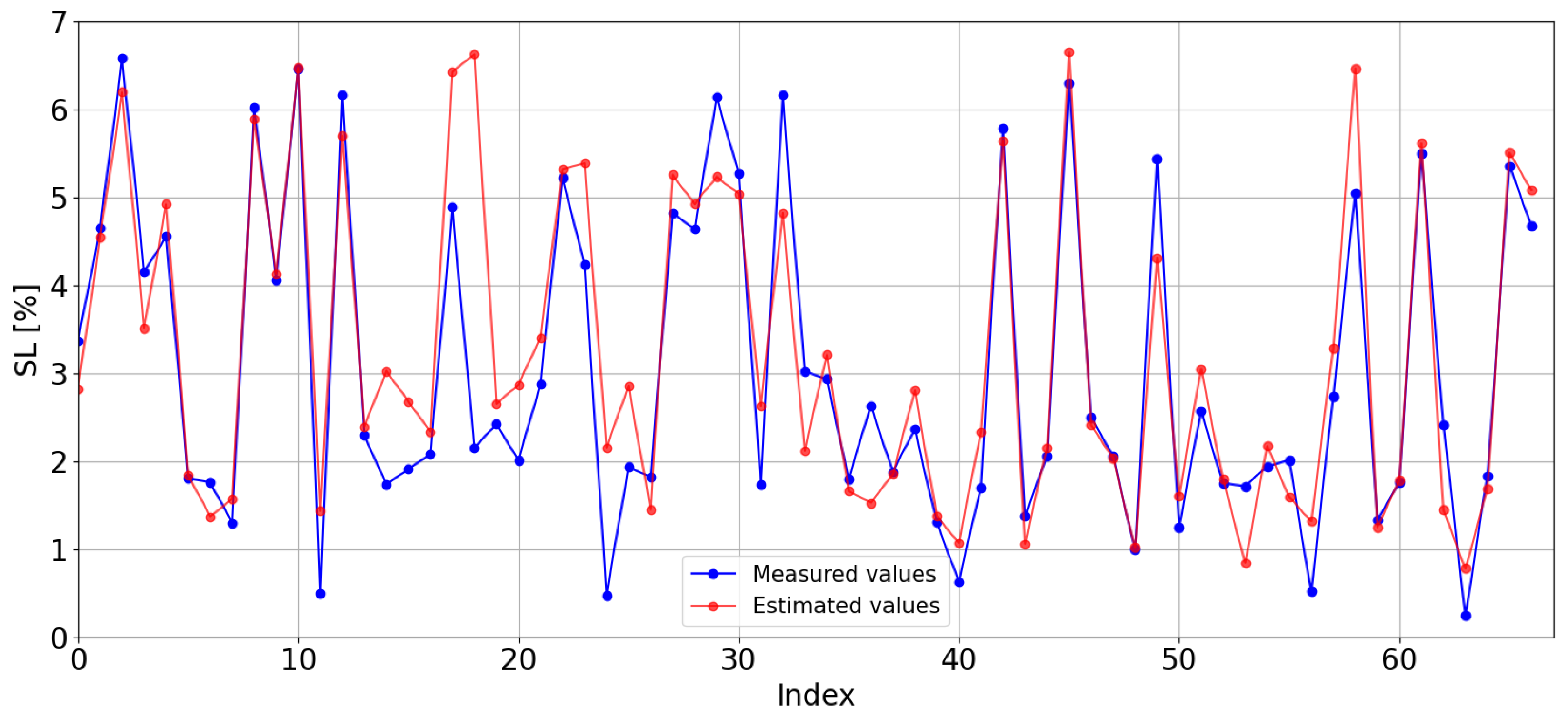
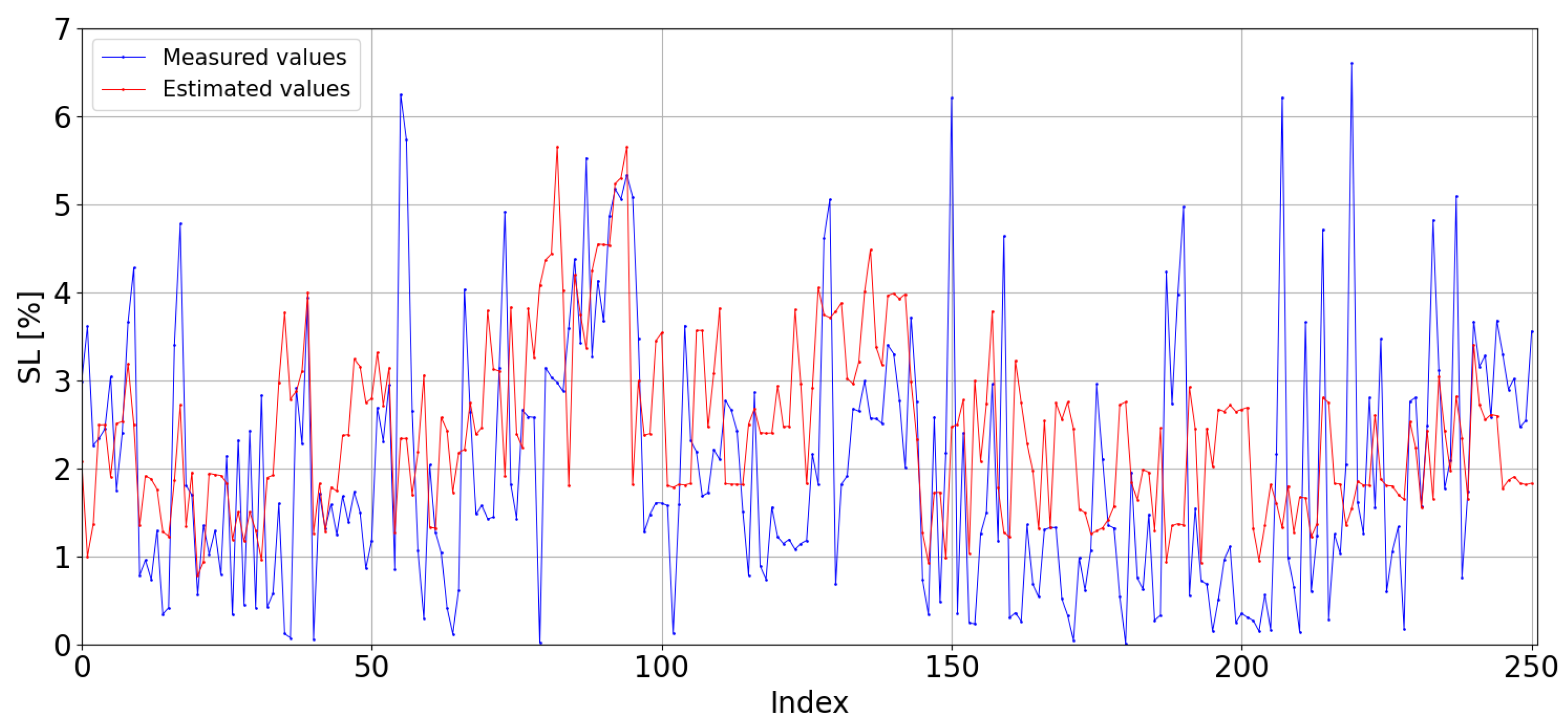
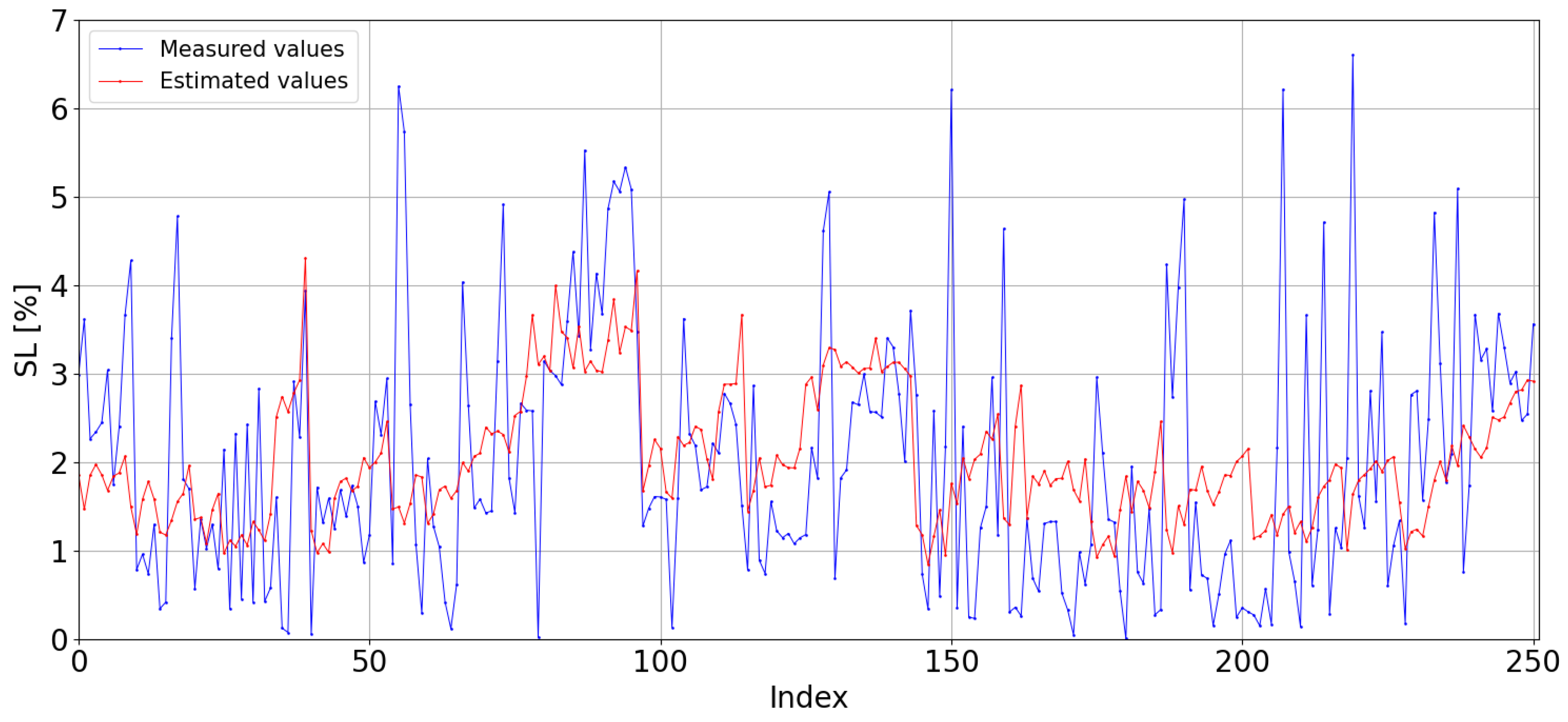
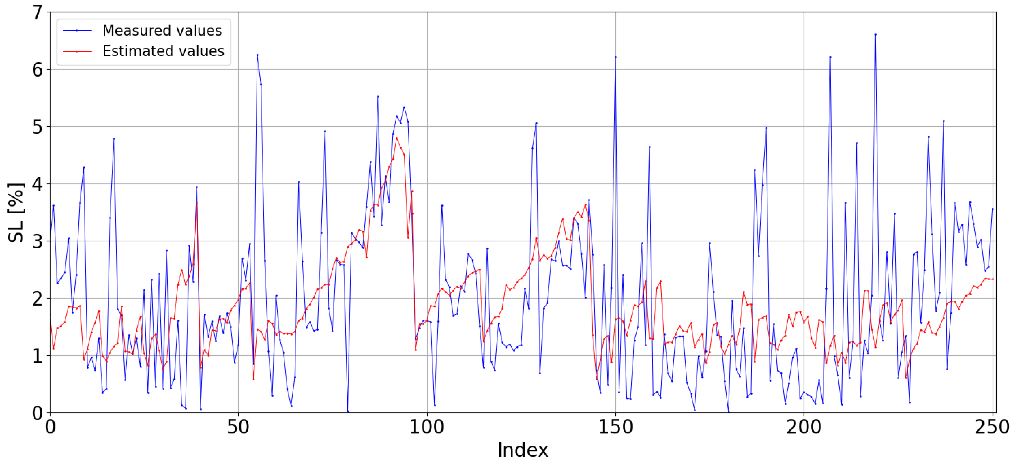
First, the estimations obtained with the kNN model trained with the data from the CIESOL station are displayed graphically along the observed (or real) values (see Figure 11) for comparison. The model tends to overestimate, with estimated values generally being higher than the observed ones, resulting in an MBE of $0.19\%$, the highest value amongst all Local Models. The RMSE is $0.84\%$ of SL.

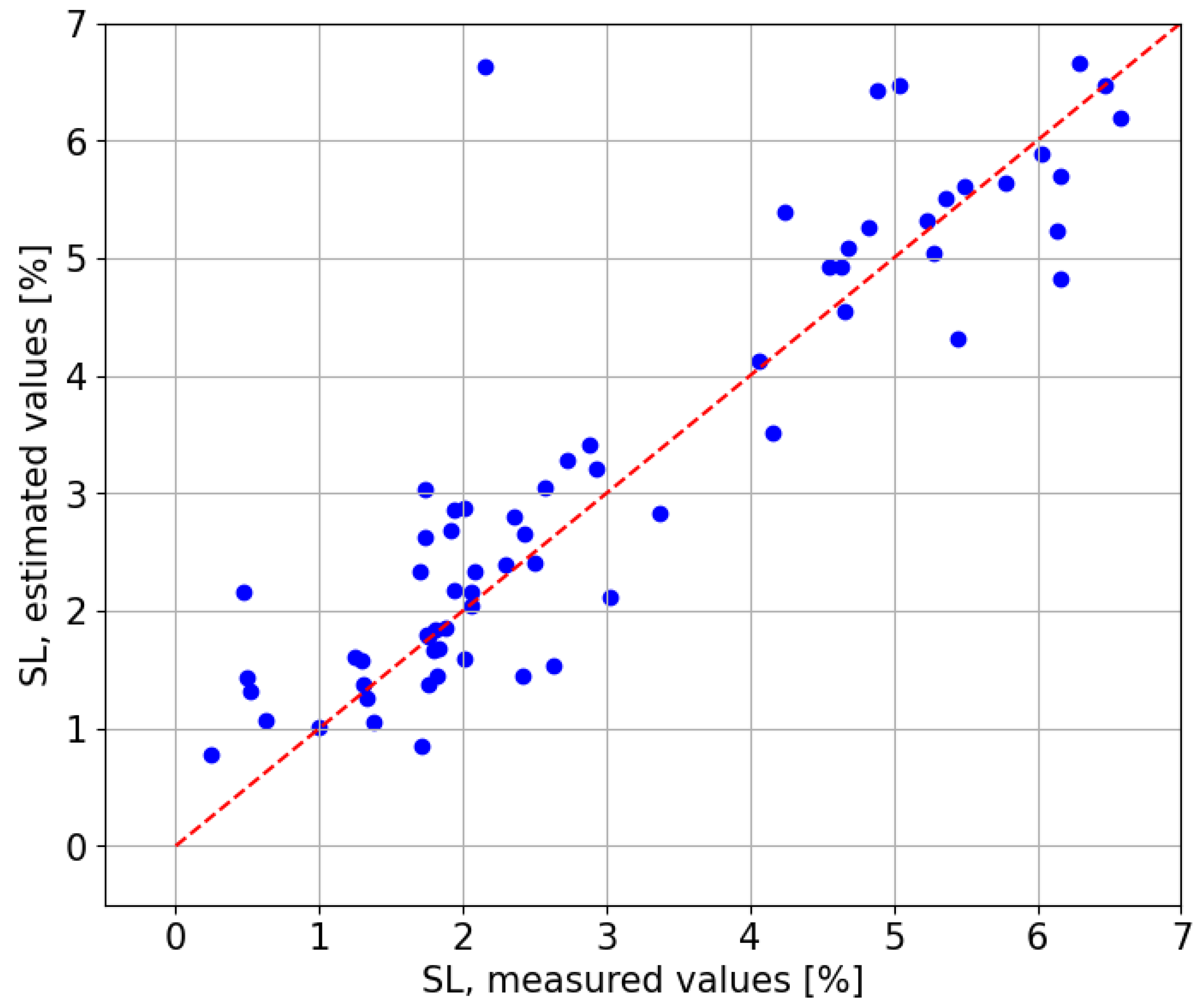
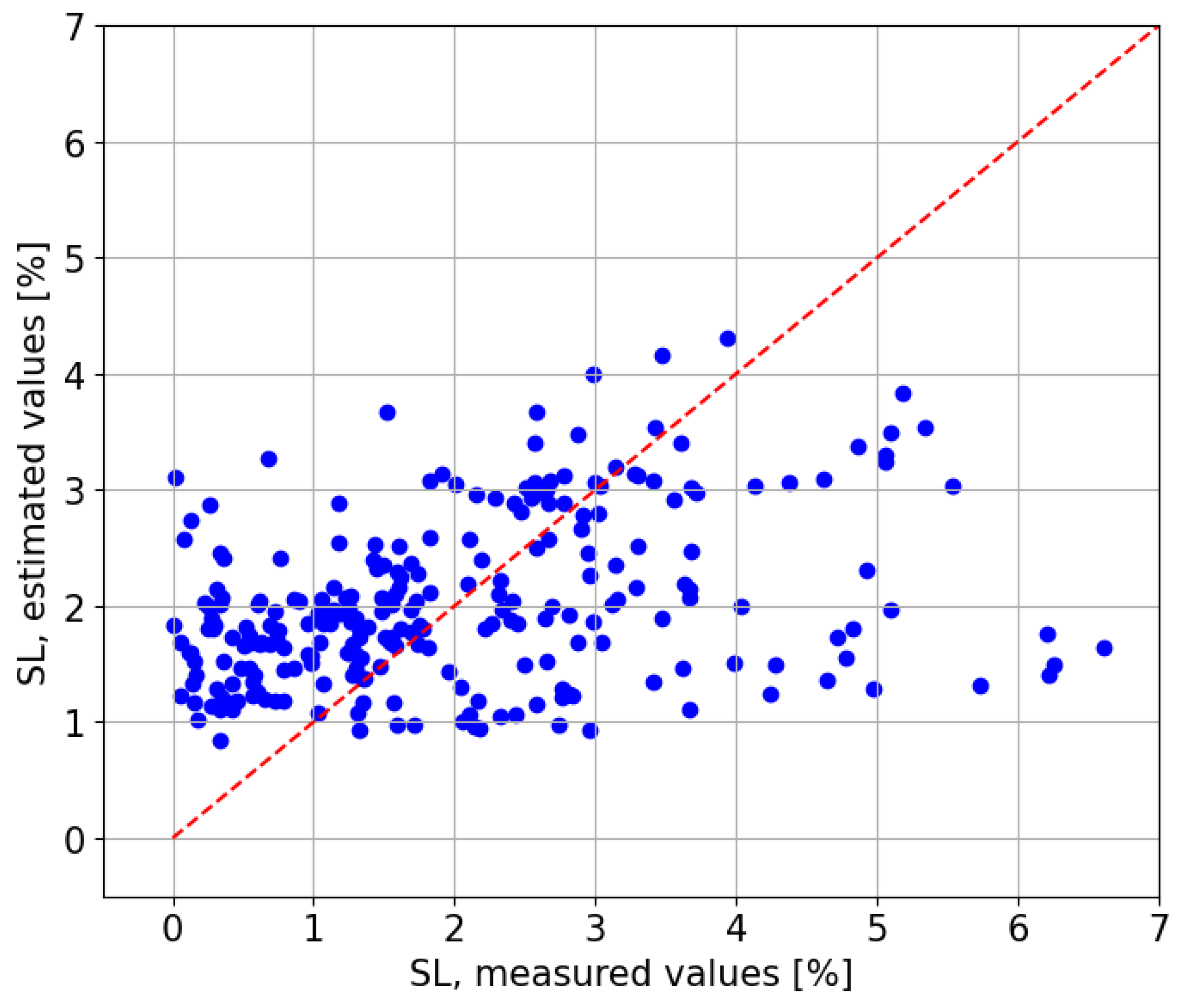
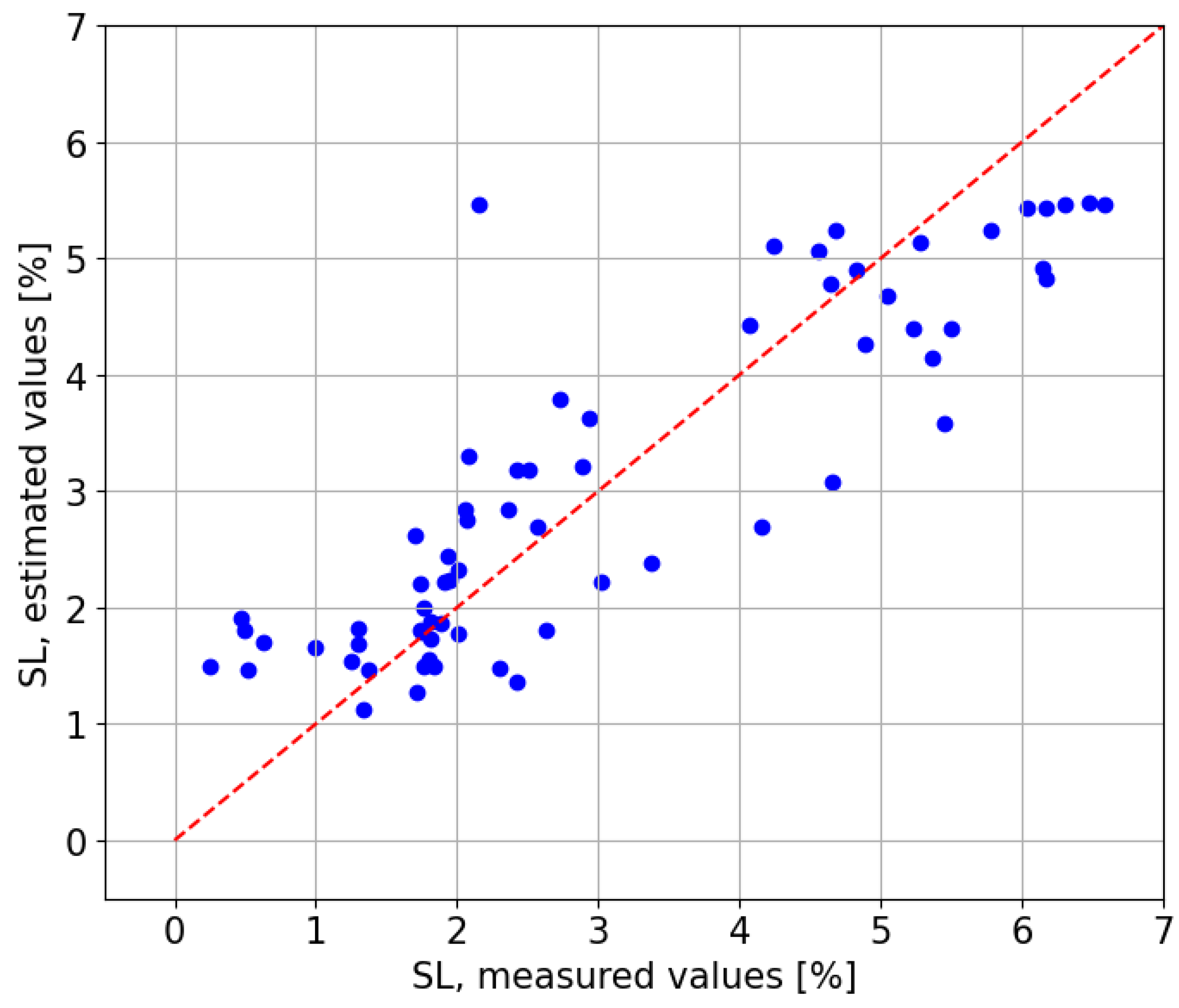
Figure 12 compares the estimated values against the observed values, revealing a clear positive relationship with a coefficient of determination of $0.78$. The red line represents the scenario in which the estimates perfectly match the observed values, which would result in an $R^2$ of 1.

3.2.2. Extrapolation of the kNN Model to the CIEMAT Test Set

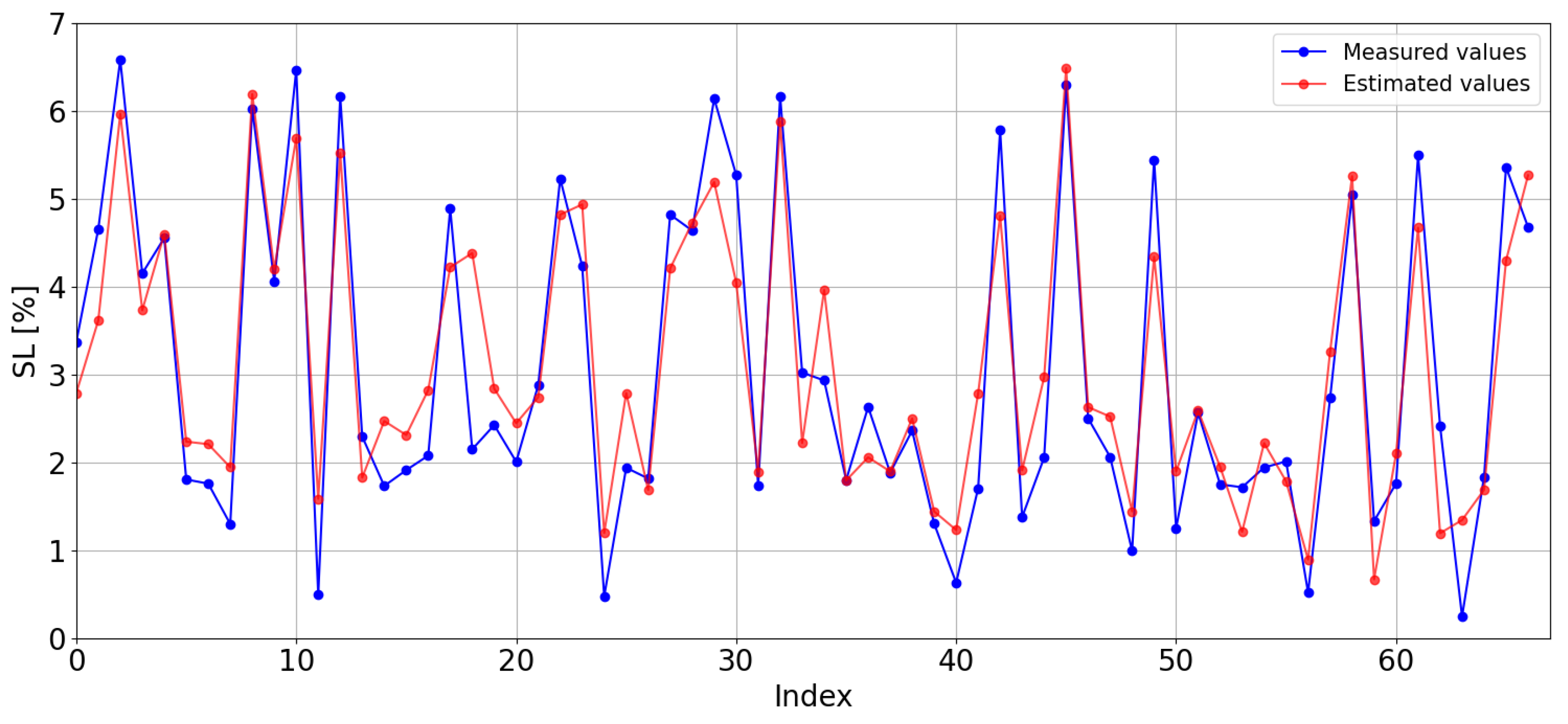
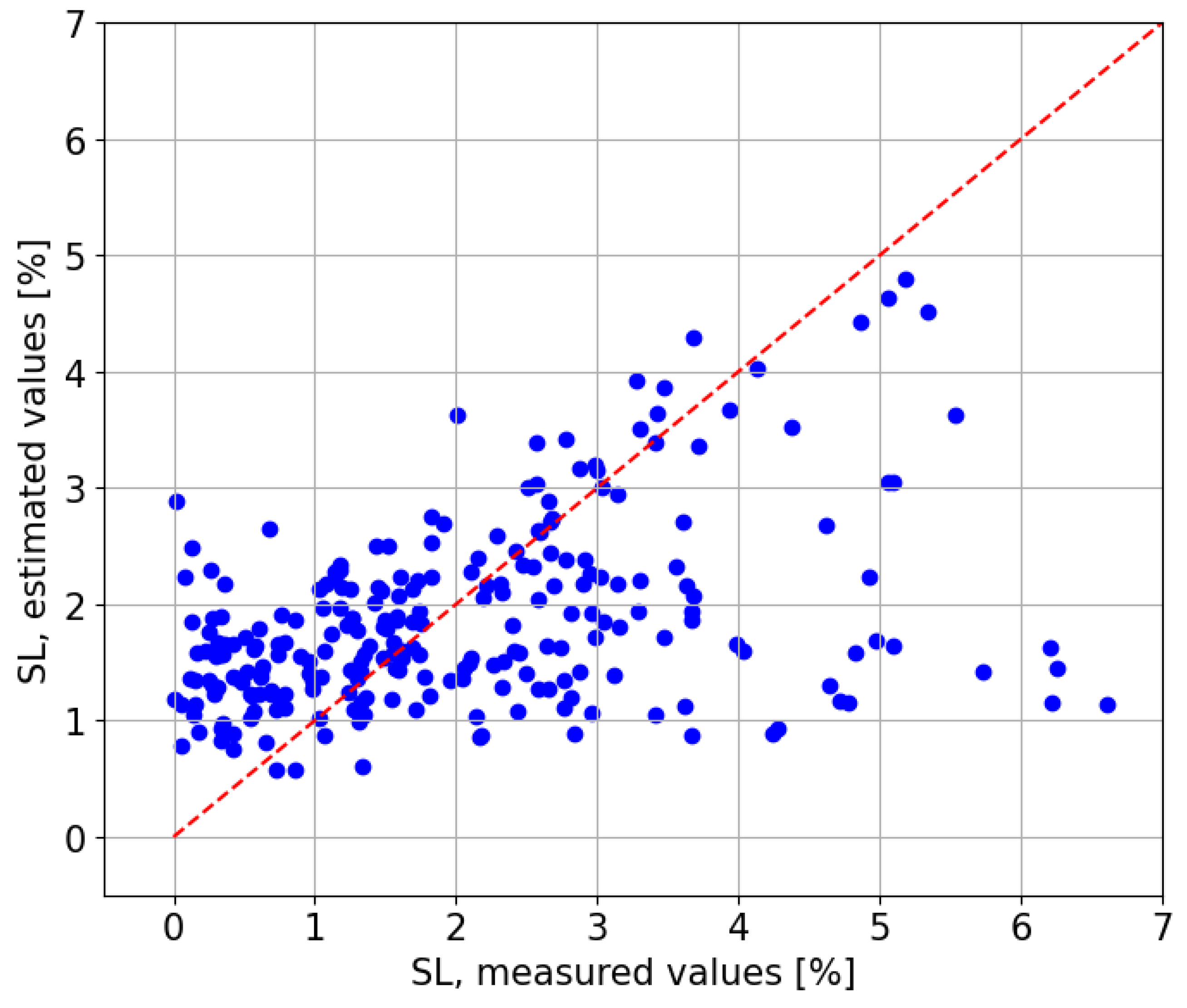
Extrapolating the kNN model to the dataset from the CIEMAT station results in an increase in both MBE ($0.39\%$) and RMSE ($1.53\%$). The model now makes greater overestimations compared to its performance on the CIESOL dataset, as seen in Figure 13.

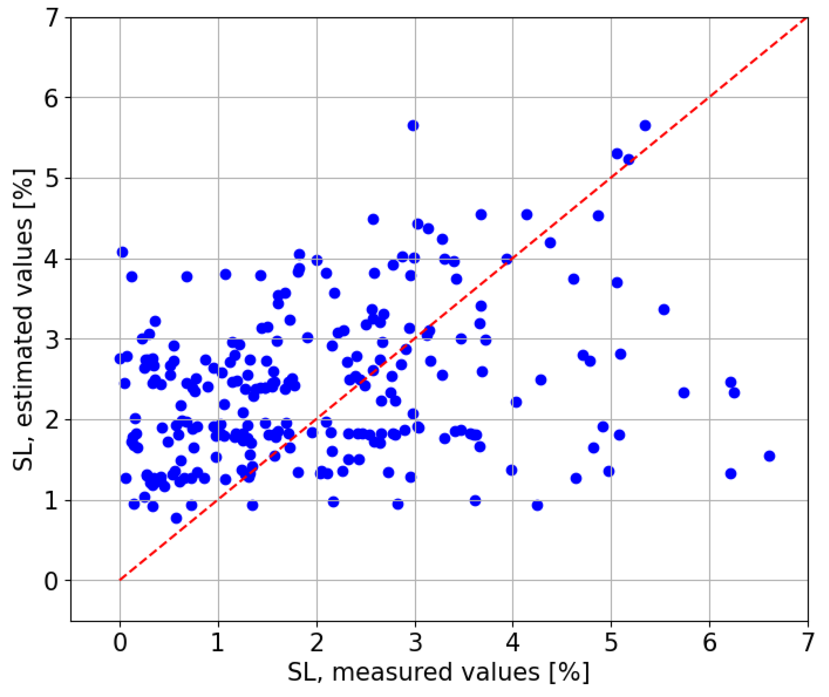
In terms of $R^2$, the model on the CIEMAT data produces a negative value of $-0.12$. This means that a predictor that always returned the mean would explain the linear regression obtained from that scatter plot (see Figure 14) better than the scatter plot itself.

3.3. Results of LightGBM Model for PV Soiling Losses Estimation

3.3.1. LightGBM Model Evaluated on CIESOL Test Set

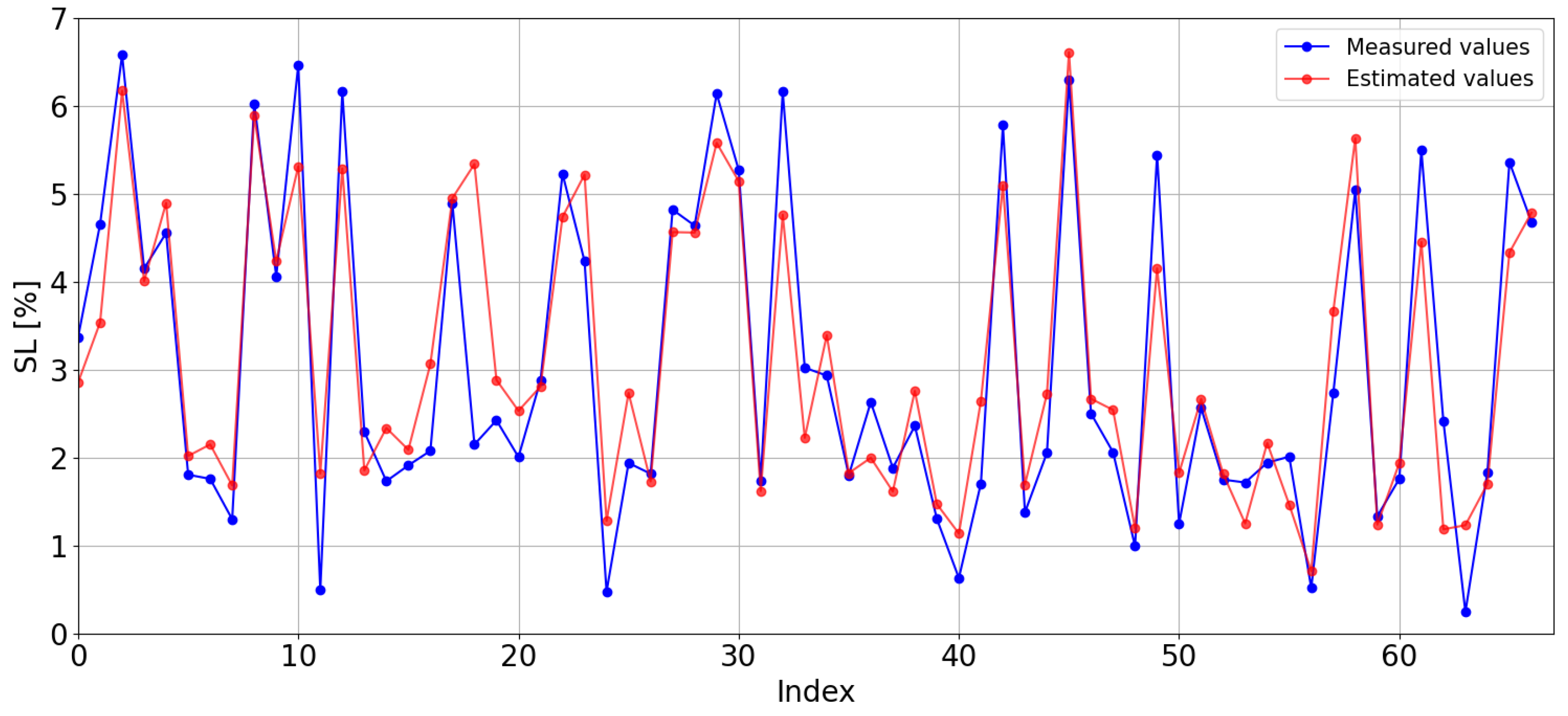
The estimations obtained with the LightGBM model trained with the CIESOL station data and the real values are shown in Figure 15. The model tends to slightly overestimate, with estimated values generally being slightly higher than the observed ones (MBE = $0.05$). The RMSE is $0.68\%$ of SL, the lowest value amongst Local Models.

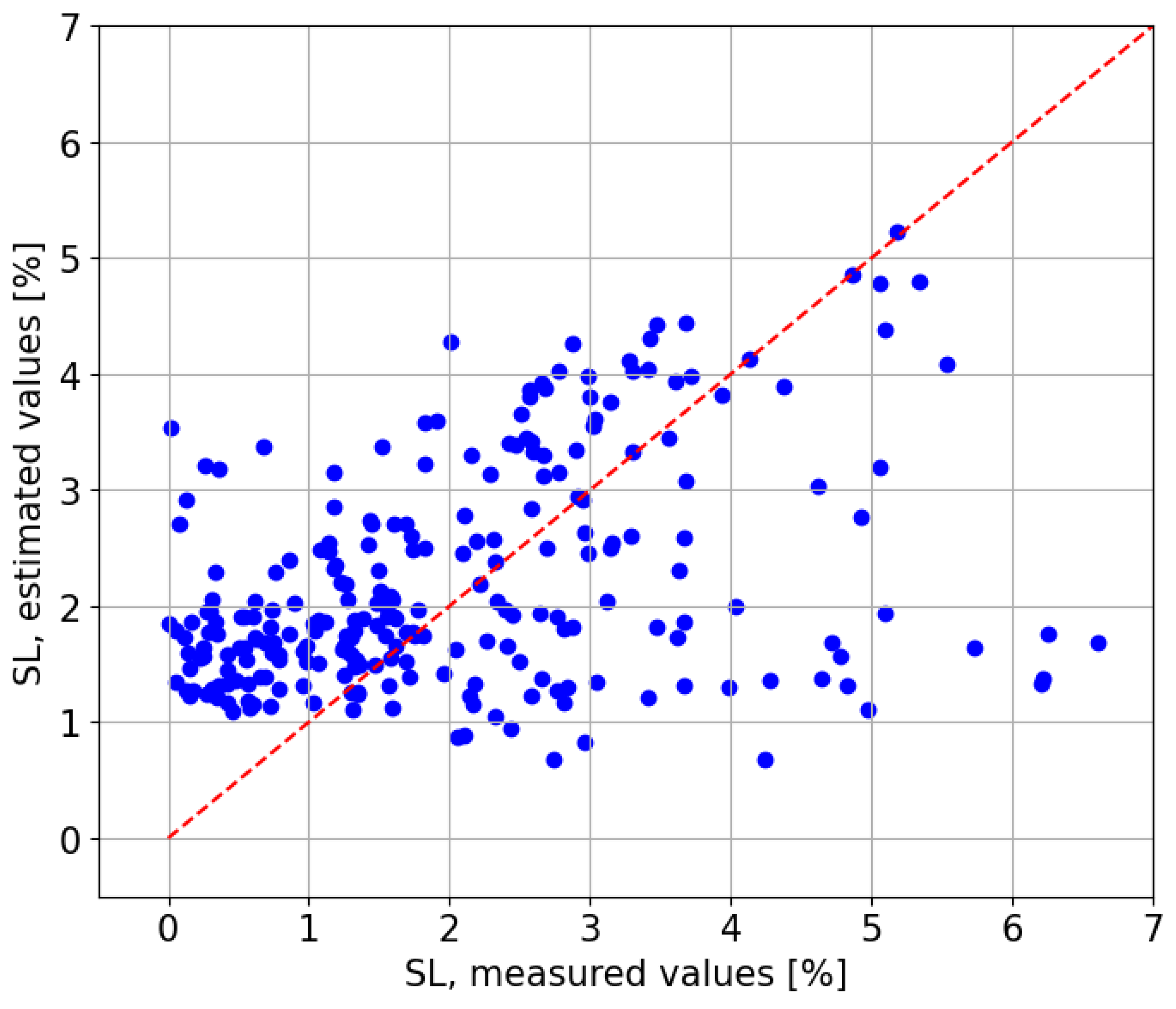
Figure 16 compares the estimated values against the observed values, revealing a clear positive relationship with a coefficient of determination of $0.86$. The red line represents the perfect fit between the real values and the estimated values.

3.3.2. Extrapolation of the LightGBM Model to the CIEMAT Test Set

The extrapolation of the LightGBM model to the CIEMAT test set results in a model that neither generally overestimates nor underestimates (see Figure 17), with a MBE of $0.02\%$, the closest value to zero amongst Extrapolated Models. The RMSE error increases significantly from $0.68\%$ obtained in the Local Model to $1.38\%$ in the Extrapolated Model (from $22.46\%$ to $68.74\%$ in normalised RMSE), the second lowest value for the ANN within the Extrapolated Model.

In terms of $R^2$, for the Extrapolated version of the LightGBM model, it shows a substantial decrease compared to the Local Model, from $0.86$ to $0.09$, resulting in a scatter plot with a weakly positive linear relationship between estimated and observed values (see Figure 18).

3.4. Results of CatBoost Model for PV Soiling Losses Estimation

Since CatBoost and LightGBM are both gradient boosting models, their structures are alike, leading to similar results.

3.4.1. CatBoost Model Evaluated on CIESOL Test Set

The estimated values obtained with the CatBoost model trained with data from the CIESOL station and the real values are displayed in Figure 19. The model tends to slightly overestimate, with the estimated values generally being slightly higher than the observed ones (MBE = $0.06$). The RMSE is $0.73\%$ of SL, the second-lowest value amongst the Local Models.

The estimated values obtained with the CatBoost model trained with data from the CIESOL station against the real values are displayed in Figure 20. The $R^2$ result is $0.83$.

3.4.2. Extrapolation of the CatBoost Model to the CIEMAT Test Set

The extrapolation of the CatBoost model to the CIEMAT test set results in a model that does not generally overestimate (see Figure 21), with a MBE of $0.19\%$, the highest value amongst Extrapolated Models. The RMSE error significantly increases from $0.73\%$ obtained in the Local Model to $1.41\%$ in the Extrapolated Model (from $24.04\%$ to $70.34\%$ in normalised RMSE), similar to the result obtained for the LightGBM model.

In terms of $R^2$ for the Extrapolated version of the CatBoost model, there is a substantial decrease compared to the Local Model, from $0.83$ to $0.05$, a weakly linear relationship between estimated and observed values (see Figure 22).

3.5. Results of the ANN Model for PV Soiling Losses Estimation

3.5.1. ANN Model Evaluated on CIESOL Test Set

The estimated values obtained with the ANN model trained with the data from the CIESOL station and the real values are displayed in Figure 23. The model neither generally overestimates nor underestimates (MBE = $0.01$), achieving the lowest value not only within the Local Models but amongst all models. The RMSE obtained is $0.88\%$ of SL, the highest value amongst Local Models, which is close to the value obtained by the kNN model ($0.84\%$).

Figure 24 compares the estimated values against the observed values, revealing a clear positive relationship with a coefficient of determination of $0.76$. The red line represents the perfect fit between real values and estimated values. This value of $R^2$ is the lowest obtained for a Local Model.

3.5.2. Extrapolation of the ANN Model to the CIEMAT Test Set

The extrapolation of the ANN model to the CIEMAT test set results in a model that largely underestimates (see Figure 25), with a MBE of $-0.15\%$, which is the lowest value amongst Extrapolated Models. The RMSE error significantly increases from $0.88\%$ in the Local Model to $1.34\%$ in the Extrapolated Model (from $29.04\%$ to $66.73\%$ in normalised RMSE), which is the lowest value amongst Extrapolated Models. Since the ANN Local Model obtained the highest errors within the Local Models and the ANN Extrapolated Model obtained the lowest errors, ANN is the model which achieves the smallest difference between models, making it the best for extrapolation.

In terms of $R^2$ for the Extrapolated version of the ANN model, it has shown a substantial decrease compared to the Local Model, from $0.76$ to $0.14$, a weak linear relationship between estimated and observed values (see Figure 26); however, it is the highest value amongst Extrapolated Models, making ANN the best model in terms of extrapolation.

3.6. Comparison with Existing Literature

This study aims to assess whether machine learning models trained on data from a specific site can reliably estimate soiling losses when applied to a different geographical location. To this end, our results are compared with previously published models, particularly those presented by Lopez-Lorente et al. in Characterizing soiling losses for photovoltaic systems in dry climates: A case study in Cyprus [26]. Their work characterizes soiling losses using both physical and machine learning models evaluated with experimental data from Nicosia, Cyprus.

In that study, physical models developed at different locations in Cyprus were tested, offering a relevant benchmark for our models trained with Madrid (CIEMAT) data. On the other hand, the machine learning models were trained and tested using a two-year dataset from Cyprus, including meteorological variables, particulate concentration, and soiling losses. The data were split 50:50 for training and testing and will be used for comparison with the models developed in this paper trained and tested with data from Almeria (CIESOL).

The physical models used in the reference study include the following:

• Kimber Model [32]: this model estimates soiling losses based on daily soiling rate, rainfall threshold for cleaning, and a post-rain grace period.
• You Model [33]: this models efficiency loss as a function of dust deposition density, based on PM concentration and number of dry days.
• Coello and Boyle Model [19]: this model incorporates PM concentration, deposition velocity, rainfall, and the tilt angle of the PV panel.

In addition, three gradient boosting algorithms were used for machine learning: XGBoost, LightGBM, and CatBoost, as described and utilised in this paper.

Table 9. Summary of normalised metrics and $R^2$ for machine learning models.

Modelo	nMBE [%]	nRMSE [%]	${\mathit{R}}^2$
Locally evaluated models
kNN CIESOL	$6.27$	$27.65$	$0.78$
LightGBM CIESOL	$\mathbf{1}.\mathbf{65}$	$\mathbf{22}.\mathbf{30}$	$\mathbf{0}.\mathbf{86}$
CatBoost CIESOL	$1.89$	$24.23$	$0.83$
ANN CIESOL	$2.07$	$31.91$	$0.71$
XGBoost (Cyprus)	$-5.86$	$64.42$	$0.37$
LightGBM (Cyprus)	$-9.24$	$68.08$	$0.39$
CatBoost (Cyprus)	$-6.68$	$59.81$	$0.47$
Extrapolated models
kNN CIEMAT	$19.56$	$76.32$	$-0.12$
LightGBM CIEMAT	$2.27$	$69.18$	$0.08$
CatBoost CIEMAT	$8.71$	$70.87$	$0.03$
ANN CIEMAT	$4.01$	$66.12$	$0.16$
Kimber (Cyprus)	$-\mathbf{0}.\mathbf{55}$	$61.01$	$\mathbf{0}.\mathbf{56}$
You (Cyprus)	$50.01$	$73.95$	$0.43$
Coello (Cyprus)	$-5.19$	$\mathbf{55}.\mathbf{57}$	$0.55$

presents the comparative results using normalized metrics: normalized mean bias error (nMBE), normalized root mean square error (nRMSE), and the coefficient of determination ($R^2$). The Kimber model achieved the best nMBE ($-0.55\%$), while the LightGBM model evaluated on the CIESOL dataset had the best performance for nRMSE ($22.3\%$) and $R^2$ ($0.86$).

Two categories of models are considered:

• Locally Evaluated Models: Models evaluated on data from the same location at which they were developed. This includes the CIESOL models and the boosting models from Cyprus. Among these, the best-performing model is LightGBM trained on CIESOL data (nMBE = 1.65%, nRMSE = 22.30%, $R^2$ = 0.86).
• Extrapolated Models: Models evaluated on data from locations different from where they were trained. This group includes machine learning models tested on CIEMAT data and the physical models (Kimber, You, and Coello) applied in Cyprus. The Kimber model stands out in this group (nMBE = $-0.55\%$, $R^2$ = 0.56), while the Coello model achieved the best nRMSE (55.57%).

Machine learning models transferred to the CIEMAT dataset experienced performance degradation, with nRMSE values ranging from 66.12% to 76.32% and nMBE from 2.27% to 19.56%. These results, however, remain comparable to the physical model metrics.

Models trained and evaluated on CIESOL data showed strong predictive performance, surpassing the machine learning models developed for Cyprus. However, when applied to new geographical contexts (CIEMAT), their accuracy decreased considerably. Nevertheless, their normalized error metrics are still comparable to those of the physical models tested in Cyprus, suggesting a promising yet limited generalization capability of machine learning approaches for soiling loss estimation.

3.7. Global Model with Data from CIESOL and CIEMAT

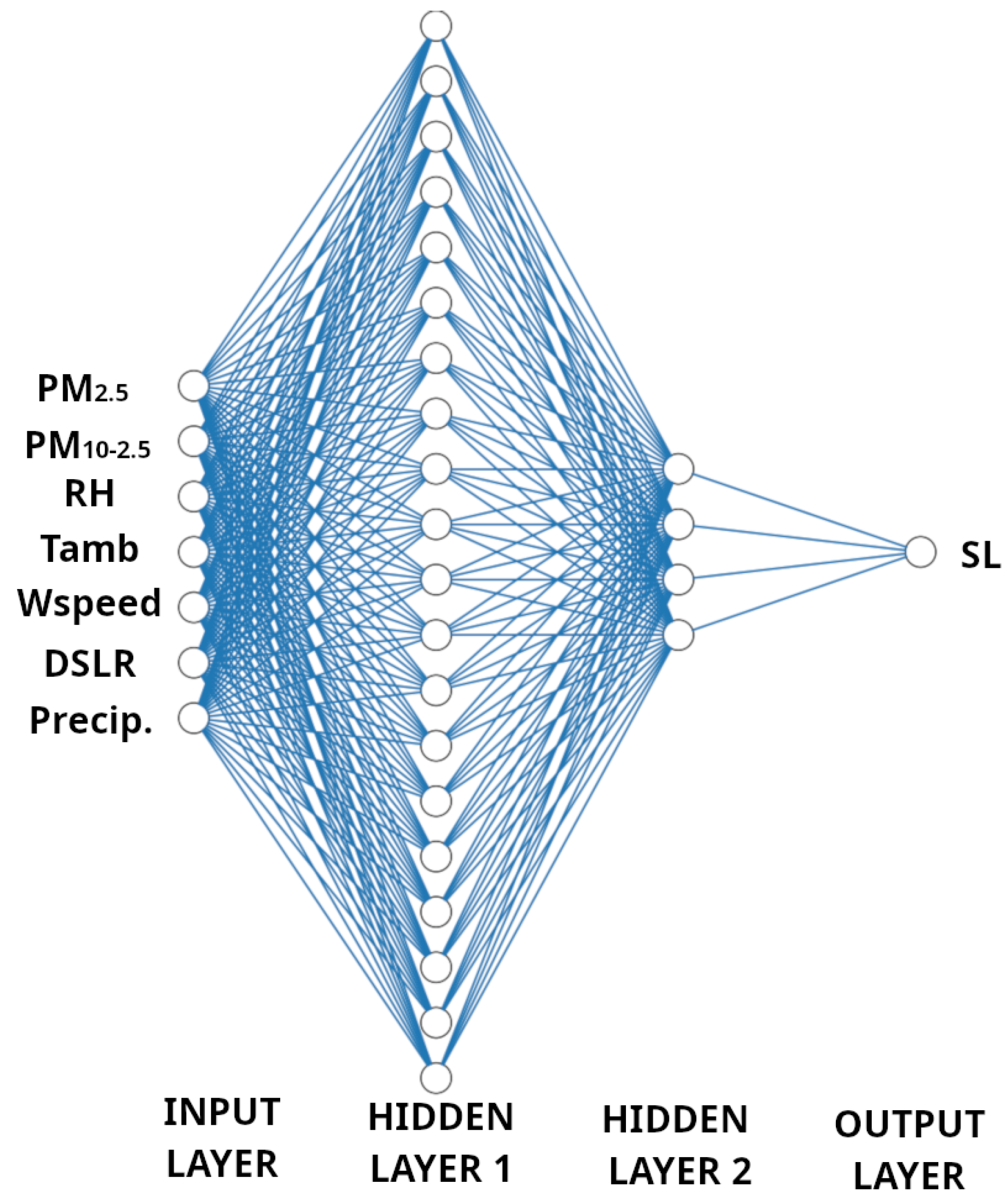
In order to develop a model capable of estimating in different locations, data from both CIESOL and CIEMAT was combined as shown in

Table 10. Train–test split for Global Model datasets CIESOL and CIEMAT.

	CIESOL	CIEMAT
Train set [days]	200	200
Test set [days]	50	50
Total days	250	250

to train an ANN following the same architecture as in Figure 27. ANN was selected for the development of the global considering that ANN achieved the best results for an Extrapolated Model.

The Extrapolated Models struggled to accurately estimate across the entire dataset range. This issue arises because the soiling patterns used for training differ significantly between locations. Specifically, in the CIESOL dataset, which was used to train the Extrapolated Models, there were very few data points where SL fell below $1\%$. In contrast, the CIEMAT test data generally exhibited lower SL values, with instances below $1\%$ being more common. As a result, the models underperformed in estimating SL values under $1\%$ (see Figure 18, Figure 22 and Figure 26), as these cases were not adequately represented in the training data. To ensure that the model learned from the entire range of soiling losses in both the training and testing datasets, stratification using binning was performed. This technique involves sorting the target variable values, dividing them into 10 bins, and then splitting the data in a way that maintains the distribution of these values in both training and test sets.

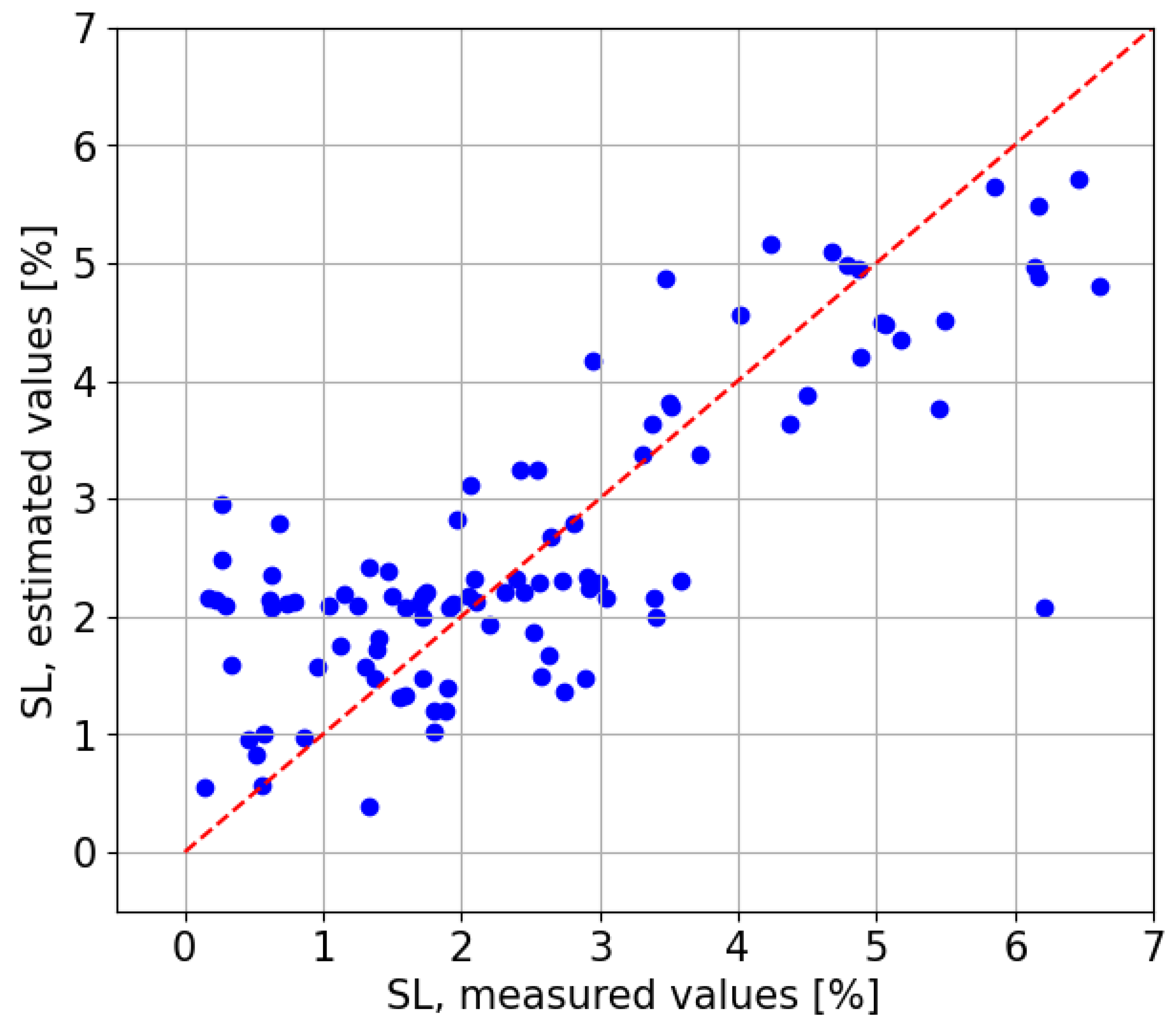
The results obtained are rather promising (see Table 8). This model achieves an MBE of $0.09\%$ ($\mathrm{nMBE}=3.41\%$) and a RMSE of $1.02\%$ (nRMSE = $40.50\%$). As for the $R^2$ between estimated and observed SLs, a coefficient of determination of $0.63$ was obtained (see Figure 28). This means that this Global Model trained with a combined dataset with data from both locations obtains a lower error than any Extrapolated Model (evaluated on CIEMAT test dataset). At the same time, $R^2$ showed similar results to the Local Models (trained on the CIESOL training dataset and tested on the CIEMAT test dataset).

4. Discussion

The primary goal of this study was to develop and evaluate machine learning models for estimating soiling losses in photovoltaic solar panels and to assess their ability to generalize across different locations. A series of machine learning models were developed and tested, including LightGBM, artificial neural networks (ANNs), and others, to determine which would provide the most accurate soiling loss estimates.

Initially, local models were trained using data from a specific site. Among these models, LightGBM demonstrated the best performance, with an RMSE of 0.68% and a normalized RMSE (nRMSE) of 22.46%. This model also showed strong predictive power with an $R^2$ value of 0.86 when comparing the observed and predicted soiling losses. These results suggest that LightGBM is effective for local estimations, especially when trained on data that reflect the particular environmental conditions of the region where the model was developed.

However, when these models were tasked with extrapolating soiling losses to a different location from the one they were originally trained on, their performance worsened, particularly in predicting soiling losses below 1%, a range that was under-represented in the original training datasets. Extrapolation, a common challenge in machine learning models, highlighted the need for a model that could generalise well across regions with varying environmental conditions. Among the models tested, the ANN stood out as the most flexible, yielding the lowest RMSE and highest $R^2$ values during extrapolation. This flexibility made it the model of choice for constructing a Global Model that incorporated data from two different datasets: CIESOL and CIEMAT.

The Global Model was developed by merging data from both datasets and applying stratification to ensure robust performance across the full range of soiling losses. It significantly outperformed the extrapolated models, which were trained on a single location and tested on another. The Global Model achieved an RMSE of 1.02%, nRMSE of 40.50%, and $R^2$ of 0.62, reflecting a significant improvement over the extrapolated models. In addition to outperforming the extrapolated models, the Global Model also demonstrated strong results when compared to well-established physical models evaluated in cross-location scenarios. For instance, the physical model developed by Coello and Boyle [19], tested on Cyprus by López-Lorente et al. [26] yielded a normalised MBE of $-5.19$ and a normalised RMSE of $55.57$, along with $R^2$ of 0.55, compared to the $3.41$, $40.40$ and $0.63$ of nMBE, nRMSE and $R^2$, respectively, achieved by the Global Model.

5. Conclusions

In conclusion, the study successfully developed machine learning models for estimating soiling losses in PV systems. The models, particularly LightGBM for local predictions and the ANN for generalization across locations, performed well in their respective contexts. Whilst local models exhibited high accuracy in their original locations, the Global Model was able to generalise better, leading to a significant performance boost in terms of RMSE and $R^2$ compared to the extrapolated models. The Global Model showed strong performance because it was trained on a more diverse dataset that included a broader range of soiling conditions. In contrast, local models, although highly accurate within their own datasets, struggled to estimate soiling values that were uncommon in their training data. For example, soiling losses below 1% were rarely present in the CIESOL dataset, making it difficult for CIESOL-trained models to perform well on CIEMAT data, where such values are more frequent. This demonstrates the Global Model’s improved ability to generalise across varying environmental contexts. Additionally, the LightGBM model demonstrated strong performance due to its ability to handle non-linear relationships and perform well with relatively small datasets, making it a robust option for soiling loss estimation.

Future work should focus on enhancing both the performance and general applicability of the proposed models, particularly the Global Model. One of the most immediate steps is to test the current Global Model in a wider range of geographic locations with different environmental conditions. This would help evaluate its ability to generalise and identify potential areas where performance may decrease due to factors that are not present in the original training data. At the same time, the development of a new version of the Global Model that incorporates training data from a broader variety of locations is recommended. Including regions with diverse climates and a wider spectrum of soiling levels would allow the model to better represent the variability of environmental influences on soiling losses. This expansion is expected to improve its accuracy and make it more robust for global applications.

In addition, the integration of Geographic Information System (GIS) tools and satellite data represents a promising direction for enhancing the capabilities of soiling loss prediction models. These external data sources can provide real-time, location-specific information on key environmental variables such as atmospheric temperature, wind speed, relative humidity, and particulate matter. Incorporating this information into the models would enable more dynamic and geographically adaptable predictions. Furthermore, since the current models are based on accessible meteorological variables, they are well suited for integration with satellite and remote sensing platforms, which can help scale their application across broader regions without the need for extensive on-site measurements.

Further exploration of LightGBM is also encouraged. This model demonstrated strong results with local data and is well suited to handling large datasets and complex interactions between variables. Additional tuning and testing with larger and more varied datasets could improve its performance even further.