A Survey of Machine Learning Methods for Time Series Prediction

Abstract

This study provides a comprehensive survey of the top-performing research papers in the field of time series prediction, offering insights into the most effective machine learning techniques, including tree-based, deep learning, and hybrid methods. It explores key factors influencing the model performance, such as the type of time series task, dataset size, and the time interval of historical data. Additionally, this study investigates potential biases in model development and weighs the trade-offs between the computational costs and performance. A detailed analysis of the most used error metrics and hyperparameter tuning methods in the reviewed papers is included. Furthermore, this study evaluates the results from prominent forecasting competitions, such as M5 and M6, to enrich the analysis. The findings of this paper highlight that tree-based methods like LightGBM 4.6.0 and deep learning methods like recurrent neural networks deliver the best performance in time series forecasting, with tree-based methods offering a significant advantage in terms of their computational efficiency. This paper concludes with practical recommendations for approaching time series forecasting tasks, offering valuable insights and actionable strategies that can enhance the accuracy and reliability of predictions derived from time series data.

1. Introduction

A Time Series Prediction is the process of predicting a future value based on historical sequential observations. Accurate predictions based on time series data play a crucial role in a wide range of domains where forecasting future values is essential for strategic planning, resource management, and decision making. The applications of time series prediction span numerous fields, including electricity consumption forecasting, environmental quality assessments (e.g., air and water quality), meteorological predictions (e.g., rainfall, solar radiation, and wind patterns), medical diagnostics (e.g., forecasting COVID-19 case trends and pneumonia incidences), traffic flow prediction, and financial domains like sales forecasting and stock market analysis.

In recent years, models based on Machine Learning (ML) have demonstrated the most success in time series forecasting and are able to generalize well to unseen data, unlike models based solely on probability and statistics. Specifically, Tree-Based Machine Learning (TBML) and Deep Learning (DL) have emerged as the most prominent approaches, excelling in scenarios where complex, nonlinear dependencies exist within the data. Their ability to generalize to unseen data makes them highly applicable to real-world problems with diverse and dynamic characteristics.

While numerous studies have examined these techniques within specific domains and several survey papers [1,2] have analyzed various approaches to time series prediction across domains, the existing literature reviews face a significant limitation. Current survey papers struggle to draw meaningful comparisons between models because they analyze independent studies, each utilizing different implementations and datasets. This heterogeneity in experimental setups prevents direct model comparisons and obscures true performance differences. This paper addresses this gap by exclusively reviewing studies that compare both TBML methods and DL approaches within the same experimental framework. By focusing on research where both methodologies are implemented and evaluated by the same researchers using identical datasets, this survey enables more robust conclusions about the relative strengths and weaknesses of these modeling approaches.

The remainder of this paper is organized as follows: Section 2 outlines the methodology employed in this survey. Section 3 reviews TBML architectures, while Section 4 examines DL architectures. Section 5 presents experimental results and discusses findings, and Section 6 highlights recent time series prediction competitions. Section 7 provides an overview of the most important takeaways of this paper, and Section 8 provides the direction for future research.

2. Methodology

A rigorous and systematic methodology is employed to identify the most relevant research papers for this survey. Web of Science is selected as the primary database because it is a trusted publisher and independent source of data with comprehensive coverage of the peer-reviewed scientific literature. Given the objective of comparing TBML methods with DL approaches in time series prediction, this paper establishes specific inclusion criteria for article selection:

• Focus on Time Series Applications: the research must address problems involving time series data;
• Utilization of Advanced TBML Methods: studies must implement advanced TBML architectures, particularly gradient-boosted decision trees or similar structures (e.g., XGBoost 2.1.4, LightGBM, or CatBoost 1.2.7);
• Utilization of Advanced Neural Network (NN) Architectures: papers must explore sophisticated NN architectures, including but not limited to recurrent neural networks (RNN), feedforward neural networks (FFNN), convolutional neural networks (CNN), long short-term memory networks (LSTM), gated recurrent units (GRU), or Transformers;
• Direct Comparisons Using Identical Datasets: the research must present comparative evaluations of at least one TBML and one DL architecture under identical experimental setups, ensuring consistent datasets and conditions.

To identify the relevant literature, a comprehensive search query is developed as follows:

(ALL = (XGBoost) OR ALL = (LightGBM) OR ALL = (CatBoost) OR ALL = (“gradient boost*”)) AND (ALL = (“time series”) OR ALL = (“time sequence”) OR ALL = (“temporal series”) OR ALL = (“temporal sequence”) OR ALL = (“time forecast*”)) AND (ALL = (“LSTM”) OR ALL = (“ANN”) OR ALL = (“CNN”) OR ALL = (“RNN”) OR ALL = (“transformer”) OR ALL = (“GRU”) OR ALL = (“deep neur*”) OR ALL = (“deep lear*”)).

This query yields 589 papers published between 2017 and 2024. To ensure focus on the most influential research, papers are initially selected based on the citation count. From the top 100 most-cited papers, 65 articles [3,4,5,6,7,8,9,10,11,12,13,14,15,16,17,18,19,20,21,22,23,24,25,26,27,28,29,30,31,32,33,34,35,36,37,38,39,40,41,42,43,44,45,46,47,48,49,50,51,52,53,54,55,56,57,58,59,60,61,62,63,64,65,66,67] satisfy the inclusion criteria. To maintain contemporary relevance and capture recent developments in the field, additional temporal criteria are implemented: a minimum of 10 papers per year from 2020 to 2024 must be included. Consequently, four highly cited papers from 2023 [68,69,70,71] and the ten most-cited articles from 2024 [72,73,74,75,76,77,78,79,80,81] are incorporated. In total, this survey encompasses 79 influential papers investigating the comparative performance of TBML and DL approaches in time series analysis.

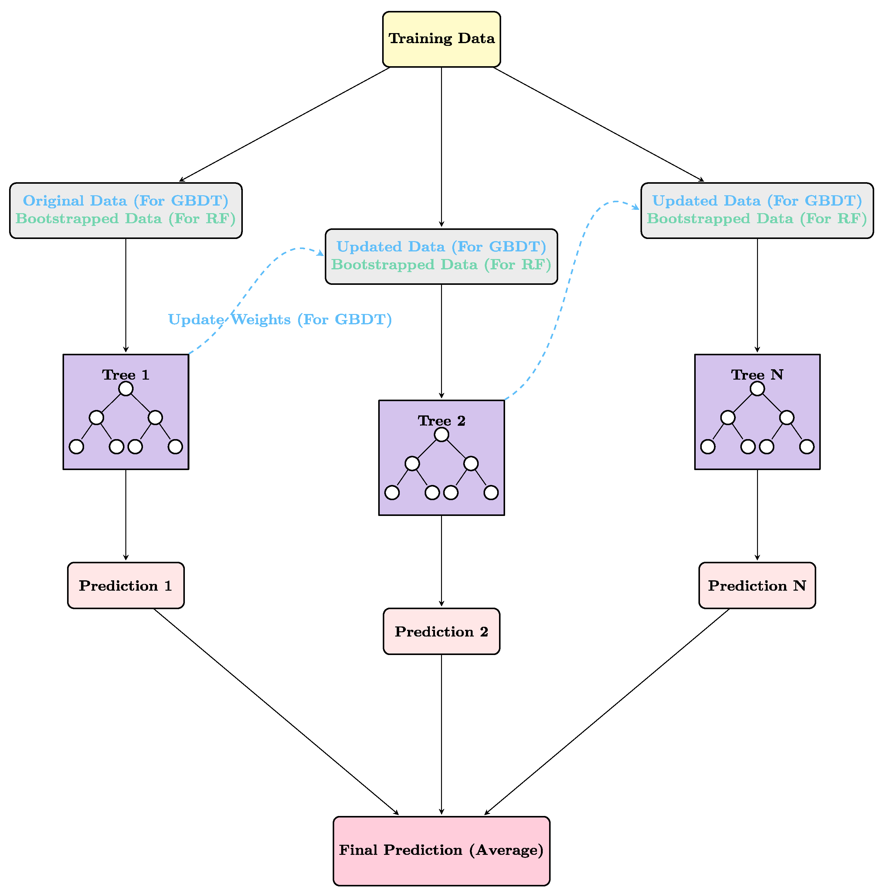
3. Tree-Based Machine Learning Architectures

This section will present an overview of the best-performing TBML Architectures, which are widely utilized for both regression and classification tasks. These include Random Forests (RF), Gradient Boosted Decision Trees (GBDT), and three prominent implementations of GBDT: XGBoost, LightGBM, and CatBoost. Figure 1 provides a comparative visualization of the structural differences between RF and GBDT. First, this study will discuss a foundational architecture in the realm of TBML: Random Forests.

3.1. Random Forests

Random Forests (RF) is an ensemble learning method that constructs multiple decision trees and combines their outputs through averaging for regression tasks or majority voting for classification tasks. RF uses bootstrapping to train individual decision trees on a random subset of the data at each split. This randomization, coupled with its ensemble nature, enhances the robustness of RF compared to single decision trees, significantly reducing the risk of overfitting.

3.2. Gradient-Boosted Decision Trees

Gradient-Boosted Decision Trees (GBDTs) are a machine learning algorithm that aggregates predictions from multiple weak learners, typically decision trees. GBDTs use “boosting” to build models iteratively, where each subsequent model focuses on correcting mistakes made by previous models. The algorithm achieves this by optimizing a differentiable loss function using gradient descent. While Scikit-learn provides a general implementation of GBDT, the three most prominent and high-performing implementations discussed in this survey are XGBoost, LightGBM, and CatBoost, each offering distinct advantages.

3.2.1. XGBoost

XGBoost, eXtreme Gradient Boosting [82], introduced by Tianqi Chen in 2014, is designed to address key limitations of traditional GBDT, particularly computational efficiency and scalability. XGBoost gained immediate popularity due to its significant speed improvements, achieved through innovative approaches in decision tree construction. Unlike the greedy splitting methods used in standard GBDT, XGBoost employs a similarity score to evaluate potential splits. This score measures the homogeneity of observations within a node relative to the target variable to asses the gain provided by a split. To further reduce overfitting, XGBoost incorporates several techniques, including pruning, where branches with a gain below a threshold (hyperparameter gamma, γ) are removed. Similarly, XGBoost has several regularization techniques that prevent overfitting by penalizing complex decision trees.

3.2.2. LightGBM

LightGBM [83], developed by Microsoft in 2017, shares many foundational principles with XGBoost with an even larger focus on the computational efficiency. LightGBM achieves a superior speed by employing histogram-based binning, which discretizes continuous features into bins, trading minor accuracy losses for dramatic speed gains. Additionally, LightGBM introduces Exclusive Feature Bundling, which is particularly effective for many real-world datasets with high-dimensional sparse features because it consolidates mutually exclusive features into a single representation. Another innovation is Gradient-Based One-Side Sampling, which prioritizes instances with large gradients while randomly sampling smaller gradients, optimizing the learning efficiency. LightGBM also utilizes a leaf-wise tree growth strategy, as opposed to the level-wise growth used in traditional GBDT and XGBoost. This approach selectively grows the leaf with the greatest potential to improve the model, enabling faster convergence and improved accuracy.

3.2.3. CatBoost

CatBoost [84], developed by Yandex in 2017, is designed with a specific emphasis on handling datasets with categorical features. One of its key innovations is a unique implementation of target encoding which takes the concept of traditional target encoding, where categorical values are replaced with the mean of the target variable for each category, and instead constructs the encoding process using only previous data to avoid data leakage. Another distinguishing feature of CatBoost is its use of symmetric decision trees, where all leaves at the same depth use identical splitting criteria. This structure not only accelerates training, but also significantly reduces the inference time, an essential advantage in some time-sensitive applications of real-world forecasting.

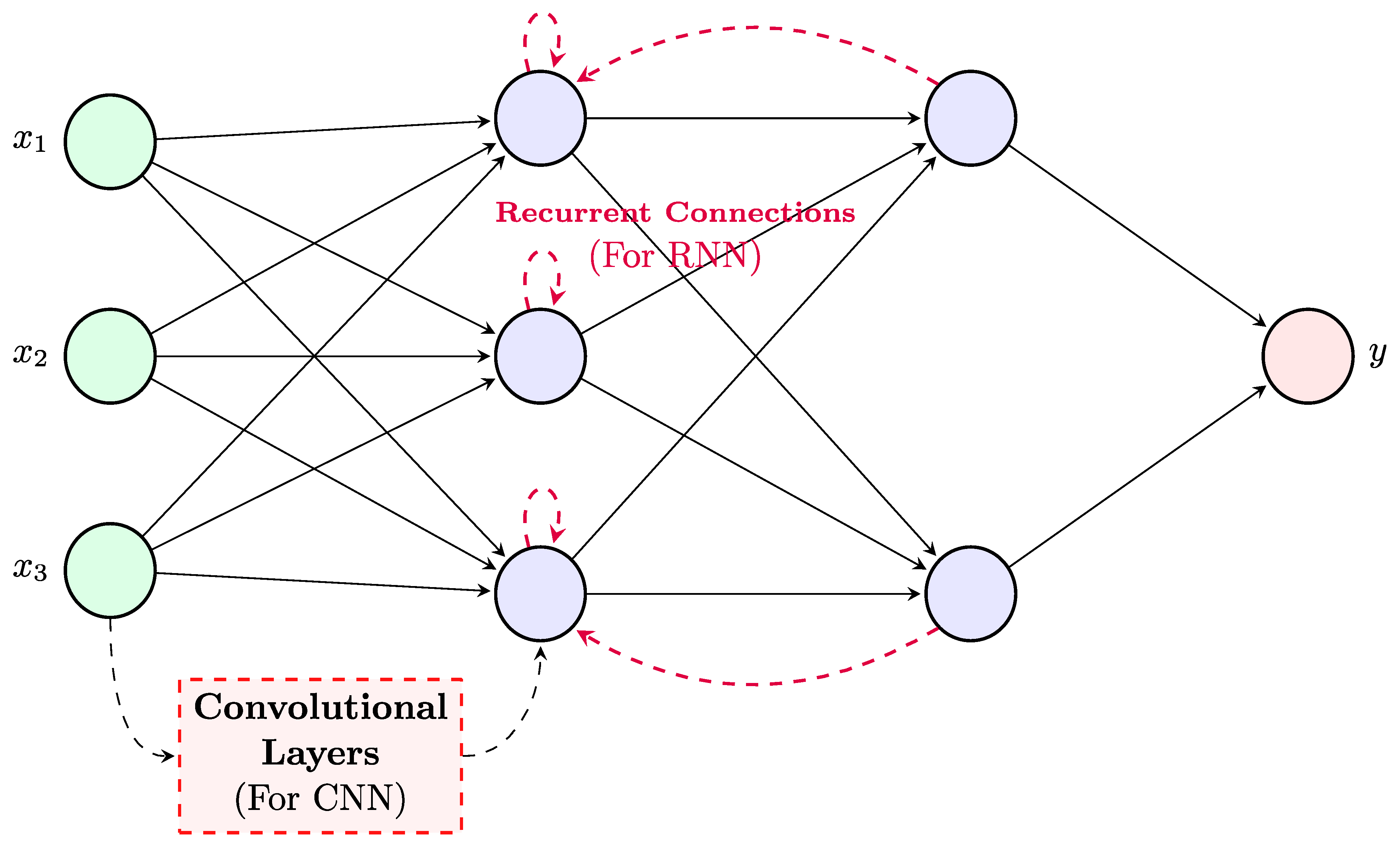
4. Deep Learning Architectures

This section presents an overview of the most prominent Deep Learning (DL) architectures encountered in the surveyed literature. DL will be used in this paper to describe a subset of machine learning that utilizes neural networks to perform classification and regression tasks. The architectures are categorized into four primary groups: Feed-Forward Neural Networks (FFNN), Recurrent Neural Networks (RNN), Convolutional Neural Networks (CNN), and Attention-based architectures. Figure 2 presents a visual representation of an FFNN, highlighting the architectural modifications required to transform it into an RNN or CNN.

4.1. Feed-Forward Neural Networks

The term Feed-Forward Neural Network (FFNN) is often used interchangeably with other terminologies in the literature, including a Artificial Neural Network (ANN), Neural Network (NN), Multilayer Perceptron (MLP), Back Propagation Neural Network (BPNN) [45,65], Deep Neural Network (DNN), and Deep Feed-Forward Neural Network (DFFNN). These networks are characterized by a unidirectional flow of information from input to output nodes, often traversing one or more hidden layers (for a comprehensive overview of the implementation details and mathematical foundation of FFNNs, see [85]).

Although the various terms for the FFNN are used interchangeably in the surveyed literature, there are small architectural differences that exist between these variants, namely in their depth. General FFNN models do not require any hidden layers, whereas MLP models typically contain one or two hidden layers. DNNs usually incorporate multiple hidden layers, allowing them to capture more complex patterns in the data. Despite their widespread use in time series analysis, these architectures require careful feature engineering to incorporate temporal information effectively and struggle to learn long-term patterns within the data. These limitations create the need for more specialized architectures including Convolutional Neural Networks (CNNs) and Recurrent Neural Networks (RNNs).

Convolutional Neural Networks

Convolutional Neural Networks (CNN) are a type of FFNN that distinguish themselves in their architectural design through convolutional layers. The biggest benefit of these convolutional layers is to systematically scan input data to extract various features, making them well-suited candidates for handling image data as they can detect local features, combine them into complex patterns, and still maintain spatial relationships between features (for a comprehensive examination of CNN architectures, including detailed mathematical formulations and implementation considerations, see [86]). Although this can be useful in certain datasets which contain a time series of images, CNN models lack the ability to remember information over longer periods of time, such as Recurrent Neural Network (RNN) models and Transformer models.

4.2. Recurrent Neural Networks

Recurrent Neural Networks (RNN) distinguish themselves through their unique feedback loop architecture, where outputs from previous timesteps are fed back into the network, creating an internal memory state that enables learning from past inputs. This recursive processing allows RNN models to incorporate historical information into current computations, making them particularly well-suited for time series analysis, where current predictions often depend heavily on historical patterns.

Among RNN variants, Long Short-Term Memory (LSTM) networks have emerged as the most popular in the literature studied for this paper, largely due to their sophisticated gating mechanisms that help mitigate the vanishing gradient problem prevalent in general RNNs. LSTM models incorporate an input, forget, and output gate to regulate the information flow and enable the network to capture both long-term dependencies and short-term patterns effectively [87]. Variants such as Bidirectional LSTMs (Bi-LSTMs), which process sequences in both forward and backward directions, enhance the model’s ability to leverage contextual information from both past and future timesteps. Another notable RNN variant is the Gated Recurrent Unit (GRU), which simplifies the LSTM architecture by combining the input and forget gates into a single update gate and introducing a reset gate. GRUs are computationally more efficient than LSTMs, while retaining a comparable performance in capturing sequence dependencies.

4.3. Attention-Based Architectures

Attention-Based Architectures, particularly Transformer Models [88], are the least explored deep learning approach among the surveyed literature in time series applications. Unlike RNNs, which use recurrent layers to process data sequentially, Transformers use a self-attention mechanism to identify ways that distant data features in a series are related to each other. They operate by processing entire sequences in parallel, making them much faster to train than RNNs. The application of Transformers has mainly been used for Natural Language Processing (NLP) models and less so for time series applications. Among the surveyed literature, only five papers [28,33,70,74,77] explore attention-based models in this domain. Early results suggest that Transformers can outperform traditional RNN-based models in tasks requiring long-term dependency modeling, though their suitability for specific time series tasks warrants further investigation.

5. Experimental Results and Discussion

With the foundational TBML and DL architectures established, the following section outlines the methodology used to conduct the analysis presented in this survey. The process begins with a detailed discussion of data preprocessing in Section 5.1, where the inclusion and exclusion criteria for models are established. Section 5.2 describes the evaluation metrics employed to systematically compare the performance of different models. The results of the analysis are presented in Section 5.3, followed by an in-depth discussion of these findings in Section 5.4.

5.1. Data Preprocessing

The primary objective of this survey is to evaluate and compare the performance of DL models against TBML methods for time series prediction. To maintain the integrity and relevance of the analysis, certain models were excluded based on their consistent underperformance or lack of applicability. Linear regression (LR) models, for example, are omitted due to their poor performance across most surveyed studies, apart from a single instance of Ridge Regression that showed promising results [27]. While this exception highlights potential avenues for future research, it should be noted that other Ridge Regression examples in the surveyed literature perform poorly [61]. Decision Tree (DT) models and Support Vector Machine (SVM) models are also excluded, as they consistently underperformed relative to other methods.

Autoregressive Integrated Moving Average (ARIMA) models, including variants like Seasonal ARIMA (SARIMA), have historically been popular for time series forecasting. However, in all surveyed instances, these models are outperformed by either DL or TBML methods. Consequently, ARIMA-based models are excluded from this comparative analysis [6,19,33,36,48,51,55,59,60,62,65]. Adaboost, a tree-based ensemble algorithm developed in 1995, is similarly excluded due to its inferior performance when compared to similar modern TBML methods such as XGBoost, LightGBM, and CatBoost. In all reviewed cases, Adaboost either underperformed or matched the performance of these more advanced methods [30,64,66,73].

For this analysis, models are grouped into broader algorithmic categories to facilitate meaningful comparisons. Radial Basis Function Neural Network (RBFN) [6], Neural Network Autoregression (NNAR) [37], and Broad Learning System (BLS) [30] models are grouped with Feed-Forward Neural Networks (FFNNs), which also encompass MLP, ANN, and DNN architectures. While Convolutional Neural Networks (CNNs) are technically FFNNs, their unique operational characteristics justify separate analysis. Recurrent Neural Network (RNN) architectures, including GRU, LSTM, and Bi-LSTM, are grouped alongside DeepAR, an autoregressive recurrent neural network [78]. The TBML category encompasses XGBoost, LightGBM, CatBoost, Bagging, GBDT, and RF models.

5.2. Evaluation Metrics

To systematically compare the performance of various models surveyed in the reviewed papers, two evaluation metrics are employed. These metrics were designed to capture different aspects of the model performance. The first metric, First Place Aggregation (FPA), measures the frequency with which a model is identified as the highest-performing or tied for the highest-performing model in the surveyed studies. FPA is calculated as:

$$\mathrm{F}\mathrm{P}\mathrm{A}={\displaystyle \frac{N_{\mathrm{first}}}{N_{\mathrm{total}}}}\times 100$$

Here, $N_{\mathrm{first}}$ represents the number of times the model achieves the top rank, while $N_{\mathrm{total}}$ is the total number of evaluations in which the model is included. FPA provides a straightforward measure of a model’s dominance in performance comparisons. A key advantage of this metric is that it mitigates the influence of any poor performing models present within comparisons.

The second metric utilizes a weighted rank aggregation (WRA) approach to account for the relative performance of a model across all comparisons, not just first-place rankings. The WRA score is calculated as:

$$\mathrm{W}\mathrm{R}\mathrm{A}=1-{\displaystyle \frac{\left(N_{\mathrm{rank}}-1\right)}{\left(N_{\mathrm{total}}-1\right)}}$$

Here, $N_{\mathrm{rank}}$ denotes the model’s rank in each comparison, with one representing the top rank. $N_{\mathrm{total}}$ is the total number of models in the comparison. This metric assigns a score of one to the top-performing model and zero to the lowest-performing model, offering a nuanced perspective that accounts for varying numbers of models across comparisons. WRA is particularly valuable in scenarios where the relative performance of models varies significantly, enabling a more comprehensive evaluation of their effectiveness.

5.3. Results

5.3.1. Overall Model Performance

The first objective of this paper is to identify the models that exhibit the best overall performance across a variety of time series prediction tasks analyzed in the 79 surveyed studies. The models can broadly be categorized into two classes: Tree-Based Machine Learning (TBML) models and Deep Learning (DL) models. Figure 3 illustrates the comparative performance of these classes based on the First Place Aggregation (FPA) and Weighted Rank Aggregation (WRA) metrics.

TBML models marginally outperform DL models as a class, achieving the best performance (FPA) in 54.55% of tasks studied, with a WRA score of 0.6910. In comparison, DL models perform best (FPA) in 52.70% of tasks and achieve a WRA score of 0.6486. It is important to note that ties for the highest-performing model contribute to a combined percentage exceeding 100%. On average, TBML models outperform DL models by approximately 2.5%. However, this comparison at the class level provides only a surface-level understanding of the performance landscape. A more granular analysis is needed to assess the performance of subclasses within each category.

Figure 4 breaks down the performance of model subclasses within the TBML and DL categories for the FPA and WRA metrics. Notably, the “Attention” subclass, which exclusively comprises Transformer models, emerges as the best-performing model in three tasks, but is only evaluated in five studies. While this result is intriguing and suggests a promising avenue for further research, the limited sample size warrants caution when interpreting these findings. Consequently, this paper does not place a primary focus on attention-based models.

From the detailed subclass analysis, it is evident that the most effective algorithms for time series prediction are Recurrent Neural Network (RNN) models, primarily comprised of LSTM, GRU, and general RNN architectures, and the Specialized Tree-Based Models (SPTB) category, which includes XGBoost, LightGBM, and CatBoost. RNNs demonstrate a superior performance, ranking as the best-performing models in 61.36% of studies and achieving a WRA score of 0.7330. They are closely followed by SPTB models, which perform best in 50% of studies and achieve a WRA score of 0.6328.

To further refine this understanding, the subclasses are broken down into individual models. Figure 5 and Figure 6 present the performance of each model based on the FPA and WRA metrics, respectively. Among individual models, CatBoost emerges as the best performer across both metrics, followed by Transformers, LSTMs, and LightGBM.

However, it is important to note that like Attention-Based Transformer models, the robustness of CatBoost’s results may be limited, as it was the best-performing model in only two out of the three studies where it was evaluated. The LSTM model, on the other hand, demonstrates a strong and consistent performance, achieving FPA of 58.97% and a WRA score of 0.7222. With 39 instances of evaluation, its results are more statistically robust. LightGBM also performs well, with FPA of 58.82% and a WRA score of 0.6608, based on 17 studies. In contrast, the two weakest-performing models were MLPs and general FFNNs. Neither model achieved the highest rank in any study, and their WRA scores, 0.2265 for MLP and 0.1667 for FFNN, were the lowest among all evaluated models. Additionally, it is notable that the most frequently compared models in the surveyed papers were XGBoost, RF, and LSTM, with 47, 43, and 39 instances, respectively.

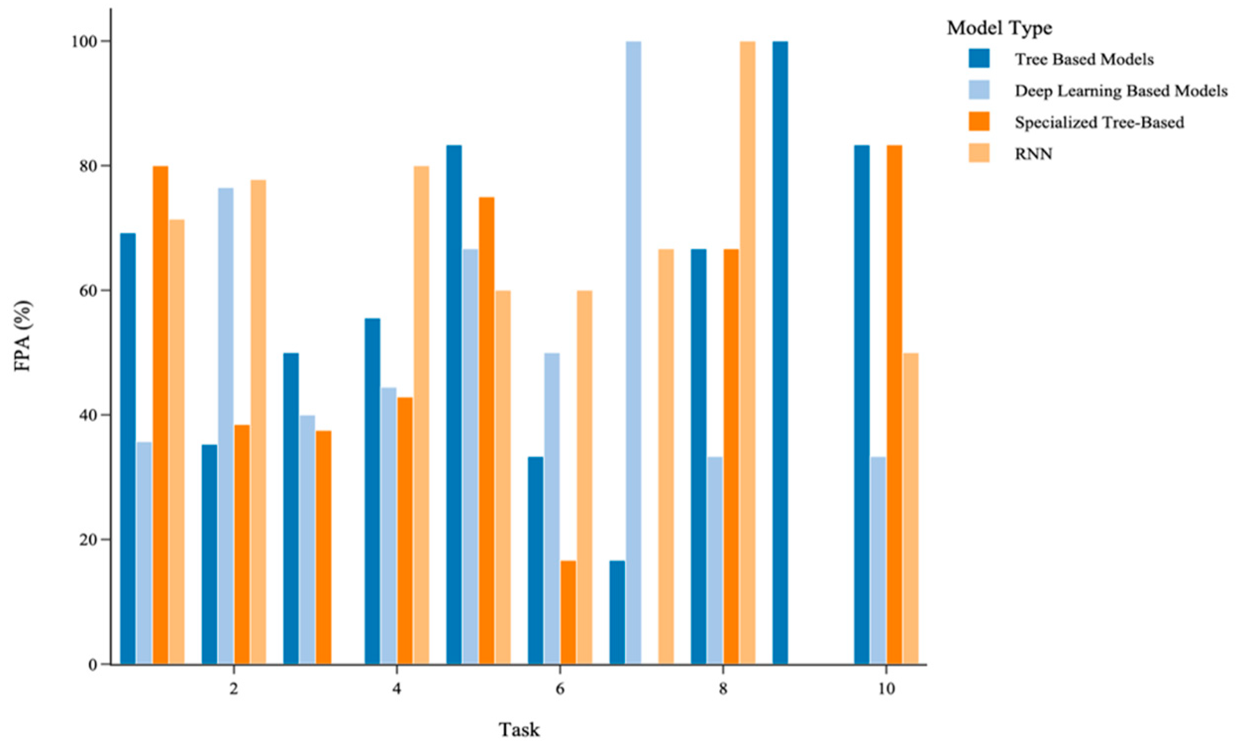
5.3.2. Task-Specific Model Performance Analysis

While overall performance metrics provide a high-level comparison of the models, they do not fully capture how each architecture performs on specific tasks. Accordingly, the next section explores the task-specific analysis of the model performance.

Table 1. Illustrates the 46 time series prediction tasks present in the surveyed papers. The frequency column shows the number of occurrences of the tasks, and the group column shows the assigned category number of each task.

No.	Time Series Prediction Task	Frequency	Group
1	Total Electricity Consumption (Demand)	8	1
2	Load Forecasting	2	1
3	Electricity Theft Prediction	1	1
4	Heating Load Prediction	1	1
5	Return Temperature of District Heating System	1	1
6	Electricity Consumption of an Electric Bus	1	1
7	Solar Power Forecasting	3	2
8	Wind Power Forecasting	2	2
9	Rainfall Prediction (Including Rainfall Runoff)	2	2
10	Drought Prediction	2	2
11	River Inflow Prediction (Including Reclaimed Water Volumes)	2	2
12	Subsurface Temperature (Including Sea Surface Temperature)	2	2
13	Reservoir Water Level Prediction	1	2
14	Flood Frequency	1	2
15	Groundwater Availability	1	2
16	Indoor Daylight Illuminances Prediction	1	2
17	Crop Yield (Including Corn Biomass, Crop Height)	5	3
18	Crop Classification	3	3
19	Water Quality Prediction (Including Chlorophyll-a and Wastewater Treatment)	8	4
20	Air Quality	1	4
21	Passenger Demand (Includes Bike Sharing, Urban Rail Passenger Flow)	3	5
22	Travel Time Prediction	1	5
23	Future Traffic of Mobile Base Stations in Urban Areas	1	5
24	Traffic Queue Length	1	5
25	Tunnel Deformation Prediction	1	6
26	Dam Structural Health Prediction	1	6
27	Highway Tunnel Pavement Performance	1	6
28	Predict Temperature Trend of Wind Turbine Gearbox	1	6
29	Discharge Capacity Estimation for Li-Ion Batteries	1	6
30	Sintering Process Prediction	1	6
31	Stock Price (Including Crypto/Stock Trend)	3	7
32	Hedge Fund Return Prediction	1	7
33	Store Item Demand	1	7
34	Vegetables Demand	1	7
35	Post-Stroke Pneumonia Prediction	1	8
36	Predict Peak Demand Days of Cardiovascular Admissions	1	8
37	COVID-19 New Cases Prediction	1	8
38	Anomaly Detection for Web Services	1	9
39	Leak Detection	1	9
40	Fall Detection	1	9
41	Global Models for Various Tasks (Simulated and Real World)	1	10
42	Predicting Emerging Research Topics	1	10
43	Lane Changing Risk	1	10
44	Predictive Process Monitoring	1	10
45	Oil Well Production	1	10
46	Crime Prediction	1	10

provides a detailed list of the 46 unique tasks covered in the surveyed papers. To facilitate meaningful comparisons, these tasks are grouped into 10 broader categories based on shared characteristics and application domains (Figure 7).

For each task category, the performance of TBML models and DL models is compared, with additional focus on the best-performing subclasses within these categories: RNNs and SPTB models. Figure 8 and Figure 9 illustrate the comparative performance of these model classes using the FPA and WRA metrics, respectively. The results highlight that TBML models consistently outperform DL models in Task Groups 1, 5, 9, and 10.

In these categories, TBML models demonstrate performance advantages ranging from 37.5% to 68.85% in WRA scores and 25% to 150% in FPA scores. Conversely, DL models show significant superiority in Task Groups 2, 6, and 7, with performance improvements of 28.57% to 97.26% in WRA and 50% to 500% in FPA compared to TBML models. A more nuanced comparison between RNN and SPTB models reveals that SPTB models perform notably better than RNNs in Task Groups 5 and 10, with WRA improvements of 45.83% and 22.22% and FPA improvements of 25% and 66.67%, respectively, compared to RNNs. In contrast, RNN models excel over SPTB models in Task Groups 2, 4, 6, 7, and 8, with performance gains compared to SPTB models ranging from 31.25% to 84.32% in WRA and 50% to 260% in FPA.

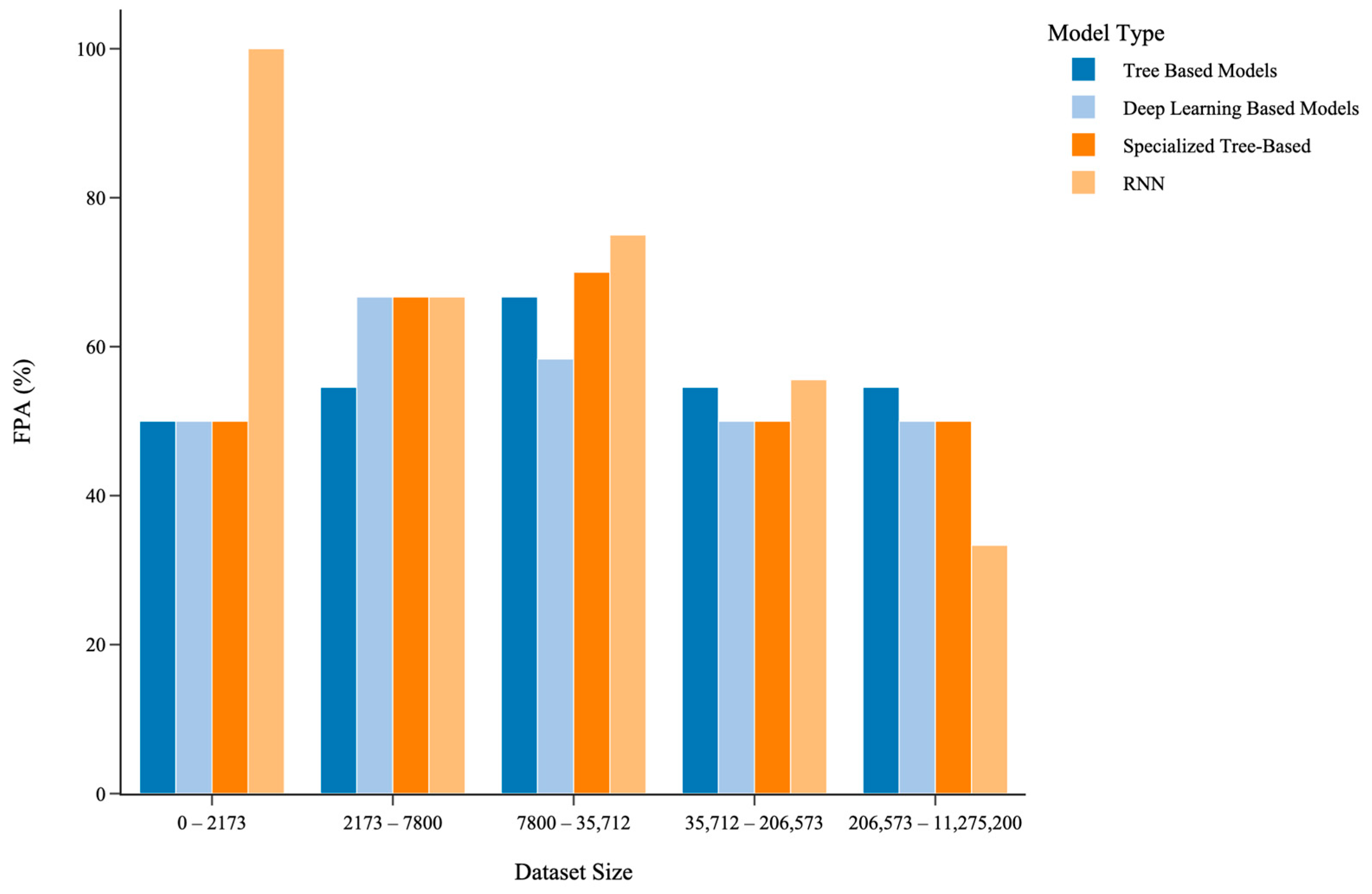
5.3.3. Impact of Dataset Size on Model Performance

Beyond examining how the model performance varies across different tasks, it is equally important to consider how external variables, such as the dataset size, contribute to these performance differences. This study also examines how the dataset size influences the relative performance of different machine learning models for time series prediction. To ensure a balanced analysis, dataset ranges were selected to contain an equal number of model comparisons within each range. The analysis considers TBML models and DL models, as well as their top-performing subclasses: SPTB models and RNNs. Figure 10 and Figure 11 present the performance of these model classes across the dataset ranges using FPA and WRA metrics, respectively.

In the smallest dataset range (0–2173 samples), TBML models perform comparably to DL models overall, but RNNs significantly outperform SPTB models, achieving an FPA advantage of 50% and a WRA advantage of 0.425. In the second range (2173–7800 samples), DL models demonstrate a slight edge over TBML models, with FPA and WRA gains of 12.12% and 0.0972, respectively. Within this range, RNNs outperform SPTB models with a WRA gain of 0.1296, while the FPA scores for both subclasses are equal.

For mid-sized datasets (7800–35,712 samples), TBML models begin to show a slight advantage over DL models, outperforming them by 8.33% in FPA and 0.0417 in WRA. However, RNN models continue to outperform SPTB models, achieving an FPA gain of 5% and a WRA gain of 0.0542. In the second-largest dataset range (35,712–206,573 samples), TBML models maintain a modest advantage over DL models, with FPA and WRA improvements of 4.55% and 0.0462, respectively. Similarly, RNNs outperform SPTB models by 0.0556 in FPA, while both achieve equivalent WRA scores. The largest dataset range (206,573–11,275,200 samples) reveals a more definitive trend. In this range, TBML models outperform DL models by 4.55% in FPA and 15.15 in WRA. Moreover, SPTB models achieve significant gains over RNN models, with an FPA advantage of 16.67% and a WRA advantage of 0.3833.

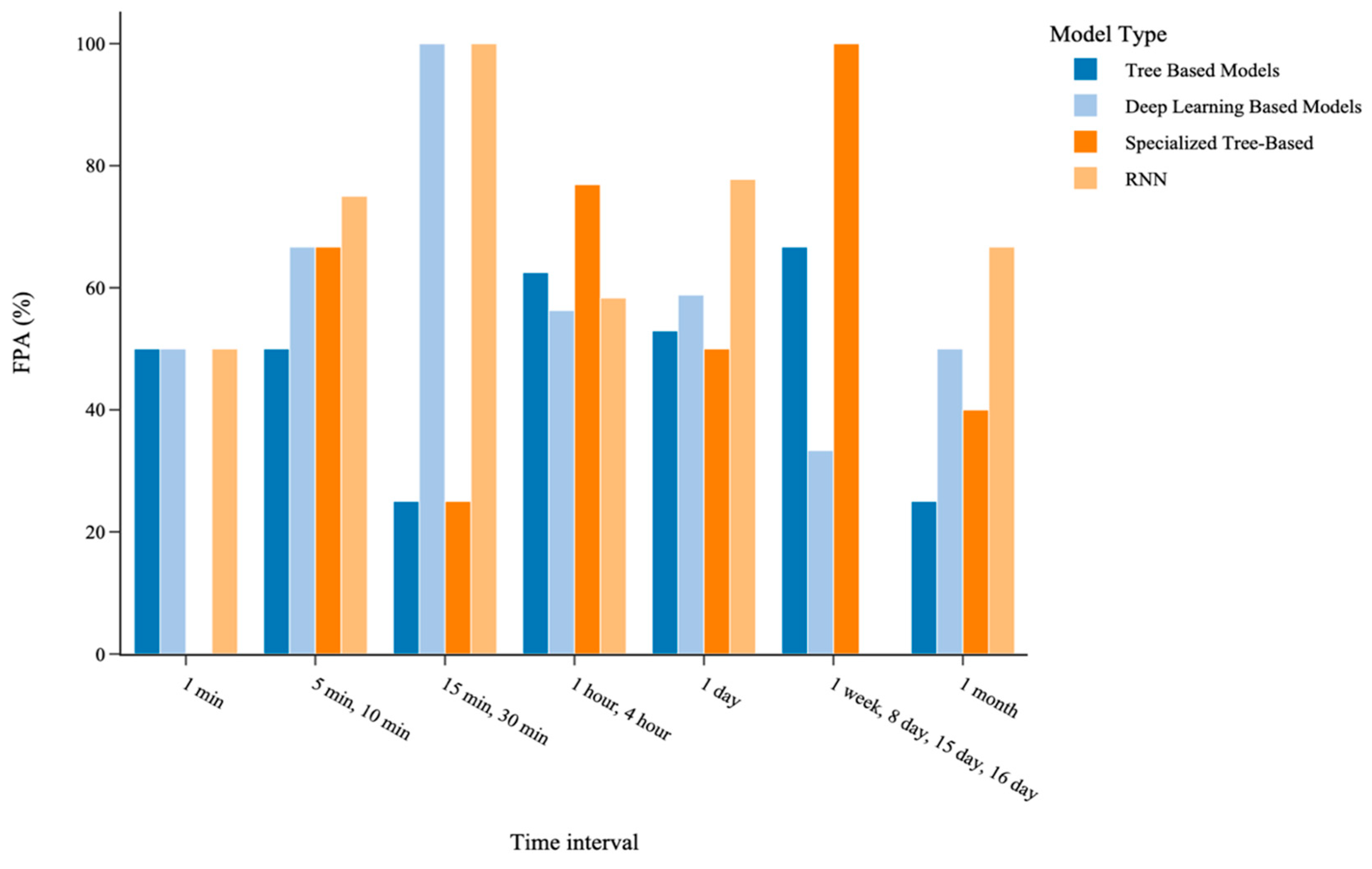
5.3.4. Impact of Data Time Interval on Model Performance

Beyond the quantity of data, this study also investigates the temporal granularity at which data are collected to explore the implications on the model performance. As in previous analyses, the comparison includes TBML models and DL models, along with their top-performing subsets: SPTB models and RNNs. Figure 12 and Figure 13 illustrate the FPA and WRA scores across different time intervals of the datasets.

DL models outperform TBML models in the 5/10 min, 15/30 min, and 1-month intervals. Notably, these intervals have a modest representation in the dataset, occurring six, four, and eight times, respectively. Conversely, TBML models show a slightly better performance in the 1/4 h interval (16 occurrences) and the 7/8/15/16-day interval (3 occurrences), with FPA and WRA advantages of 6.25% and 0.0469, and 33.33% and 0.0556, respectively. The time intervals of 8 days and 16 days are tested using the same model, see [9].

A deeper comparison of subclasses reveals that RNN models outperform SPTB models in the 1 min, 5/10 min, 15/30 min, 1-day, and 1-month time intervals. Among these, the 1-day interval (9 RNN occurrences vs. 12 SPTB occurrences) is particularly significant, where RNN models achieve a notable FPA advantage of 27.78% and a WRA advantage of 0.2509. On the other hand, SPTB models surpass RNN models in the 1/4 h and 7/8/15/16-day intervals. The 1/4 h interval (16 occurrences) is particularly noteworthy, with SPTB models outperforming RNNs by 18.59% in FPA and 0.0785 in WRA.

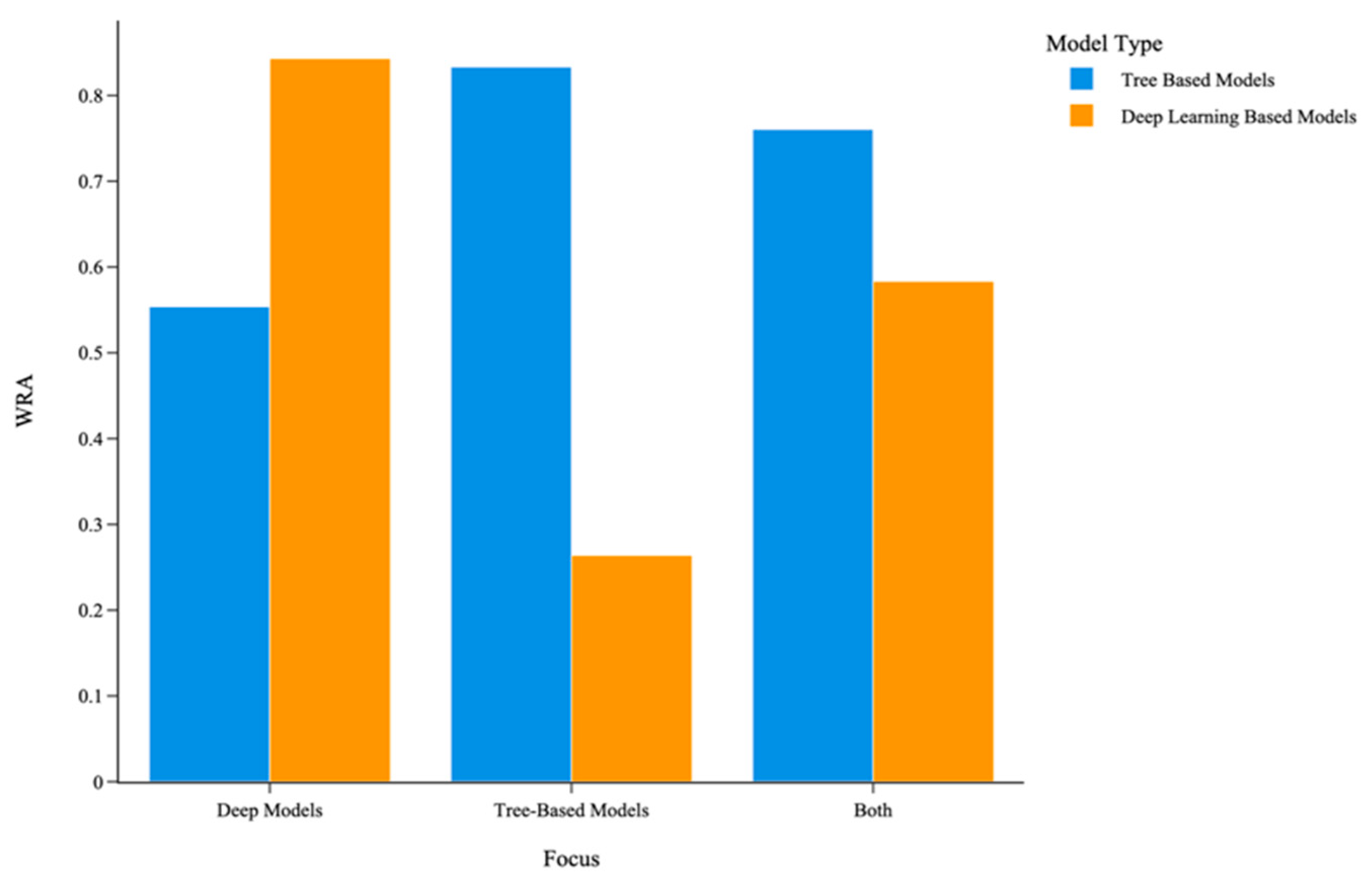
5.3.5. Impact of Research Focus on Observed Model Performance

While intrinsic data characteristics undoubtedly influence the model performance, it is also important to study how research priorities and biases shape the model performance. The papers surveyed in this study exhibit diverse objectives and emphases, ranging from developing hybrid deep neural networks to benchmarking specific advanced TBML models against DL models, or conducting balanced evaluations across a variety of ML and DL approaches. This subsection examines whether the primary focus of the research—categorized as TBML models, DL models, or a balanced approach—affects the observed performance outcomes of the evaluated models. Figure 14 and Figure 15 present the FPA and WRA scores, respectively, for TBML and DL models under each research focus category. The results reveal a noticeable bias in performance outcomes depending on the primary focus of the papers:

• Deep Learning-Focused Papers:
    When the primary focus of the paper is on deep learning models, DL models outperform TBML models significantly. The FPA score for DL models is 33.79% higher, and the WRA score is 0.2891 points higher than TBML models. This finding suggests that papers with a DL emphasis may introduce methodological, architectural, or experimental advantages tailored to highlight the DL performance.
• Tree-Based Model-Focused Papers:
    Conversely, when papers focus on TBML models, the observed performance skews in favor of TBML models. In this category, TBML models achieve a 66.67% higher FPA score and a 0.5694 higher WRA score compared to DL models. These results indicate that TBML-focused research often optimizes conditions or design choices that favor these methods.
• Balanced Focus Papers:
    In papers with no specific emphasis on either model class, TBML models slightly outperform DL models. The FPA score for TBML models is 15.23% higher, and the WRA score is 0.1771 points higher than DL models. This finding suggests that when research is conducted without bias toward a specific model class, TBML models may have a slight advantage, potentially due to their relative simplicity and robustness in a range of scenarios.

Besides exploring inherent data characteristics or potential biases that may affect a model’s performance, it is important to investigate the computational cost required to train a model.

5.3.6. Model Training Time Analysis

An essential factor to consider when evaluating the performance of ML models is their training time, particularly given the significant computational costs associated with some models. The training time directly impacts the feasibility of deploying these models in real-world applications where computational efficiency is often critical. Of the surveyed papers, ten studies [4,20,29,43,45,51,55,66,67,74] provide training time comparisons for the models evaluated. In these papers, the training time of the best-performing TBML model and DL model is analyzed.

The results demonstrate that TBML models significantly outperform DL models in terms of their training efficiency (

Table 2. TBML training advantage for each surveyed study that conducts training time analyses.

Metric	TBML Training Advantage (%)
Study [4]	4010.33
Study [20]	181.81
Study [29]	−22.55
Study [67]	1251.81
Study [43]	142.66
Study [45]	7196.53
Study [74]	905,140
Study [51]	235,559.39
Study [55]	10,145.98
Study [66]	100,140
Median	5603.43
Mean	126,934.94

). Notably, there is only one instance [29] where a DL model, an MLP, trained faster than its TBML counterpart (XGBoost). In this specific case, the MLP achieved a 22.55% reduction in its training time compared to XGBoost. However, across all ten studies, TBML models demonstrated a marked advantage. On average, TBML models were 126,934.94% faster than DL models, with the median training time advantage being 5603.43% faster. This stark difference underscores the efficiency of TBML models in scenarios where computational resources and time constraints are limiting factors.

In order to assess the impact of data characteristics and computational efficiency differences between models, it is important to analyze how these model performances are quantified in the first place.

5.3.7. Analysis of Error Metrics in Model Evaluation

Evaluating the model performance requires the use of appropriate error metrics, which vary depending on whether the task involves classification or regression. This subsection provides a comprehensive analysis of the error metrics employed across the surveyed papers.

Error Metrics for Classification Models

The classification models reviewed in this study were evaluated using the following set of metrics:

• False Positive Rate (FPR);
• Kappa Coefficient (KC);
• Positive Predictive Value (PPV);
• Negative Predictive Value (NPV);
• Receiver-Operating Characteristic (ROC) Curve;
• Matthews Correlation Coefficient (MCC);
• Area Under the ROC Curve (AUC);
• Sensitivity;
• Specificity;
• Recall;
• Precision;
• F1 Score;
• Accuracy.

The frequency of these metrics’ usage is illustrated in Figure 16. The metric names are reported exactly as listed in the surveyed papers, even if some represent equivalent measures (e.g., recall and sensitivity).

Among the most employed metrics, Recall was used in 35.29% of the studies, Precision in 41.18%, the F1 Score in 47.06%, and Accuracy in 76.47% of the papers.

Error Metrics for Regression Models

The regression models reviewed in this study were evaluated using the following set of metrics:

• Index of Agreement (IA);
• Normalized Mean Absolute Percentage Error (NMAPE);
• Prediction of Change in Direction (POCID);
• Mean Normalized Bias (MNB);
• Normalized Mean Bias Error (NMBE);
• Root Mean Squared Percentage Error (RMSPE);
• Root Squared Logarithmic Error (RMSLE);
• Mean;
• Percent Bias (PBIAS);
• R;
• Mean Absolute Scaled Error (MASE);
• Symmetric Mean Absolute Error (SMAPE);
• Coefficient of Variation of the Root Mean Square Error (CVRMSE);
• Nash–Sutcliffe Efficiency (NSE);
• Domain-Specific Error Metrics;
• Mean Squared Error (MSE);
• Mean Absolute Percentage Error (MAPE);
• R²;
• Mean Absolute Error (MAE);
• Root Mean Squared Error (RMSE).

The prevalence of these metrics is depicted in Figure 17. Among the traditional metrics, MSE was used in 22.03% of the papers, MAPE in 37.29%, R² in 45.76%, MAE in 55.93%, and RMSE in 67.80%.

5.3.8. Hyperparameter Optimization Techniques

Hyperparameter tuning is another critical aspect of ML model development, as the choice of hyperparameters can significantly influence the performance. Several of the surveyed articles specify the hyperparameter optimization techniques employed in their studies. Figure 18 illustrates the relative prevalence of these techniques across the surveyed papers. The most used hyperparameter optimization technique was a Grid Search, followed by Bayesian Optimization (BO), Random Search, Manual Optimization, and OPTUNA Automatic Hyperparameter Tuning Software. Less frequently used methods included algorithms such as the Firefly Algorithm (FA) [21], Neural Network Intelligence (NNI) [33], Enhanced Reptile Search Algorithm (ERSA) [73], and Hidden Dipper Throated Optimization (HDTO) [78], each of which was mentioned in only one paper. While many studies focused on a single optimization approach, one paper [45] provided a comparative evaluation of multiple hyperparameter optimization methods. This study found that Bayesian Optimization outperformed techniques such as a Grid Search and Particle Swarm Optimization (PSO) in terms of its search effectiveness. By leveraging probabilistic models to guide the search process, Bayesian Optimization was able to reduce computational costs while identifying optimal hyperparameter configurations more efficiently.

Having examined the performance of conventional model architectures, this study now shifts focus to hybrid models, which integrate multiple ML and DL architectures, and are a common approach to improving the predictive performance in time series tasks.

5.3.9. Comparative Analysis of Hybrid Models

Across the surveyed literature, hybrid models often outperform individual stand-alone models, although there are notable exceptions. This section examines these exceptions as well as provides insights into the relative performance of different hybrid configurations.

Performance of Hybrid Models vs. Individual Models

While hybrid models generally exhibit a superior performance, a few studies highlight cases where individual models outperform hybrids:

• Study [44]: a 2D CNN, 3D CNN, and XGBoost model each outperformed a hybrid RNN-CNN model;
• Study [80]: RF and XGBoost models surpassed multiple hybrid models, including CNN-LSTM, CNN-GRU, RNN-GRU, and RNN-LSTM configurations;
• Study [81]: a CatBoost model outperformed a spatio-temporal attention-based CNN and Bi-LSTM hybrid model.

Hybrid Models Compared to Other Hybrids

Several papers explored the relative performance of different hybrid configurations, providing valuable insights into the design considerations:

• Study [45]: a hybrid CNN-LSTM-Attention model outperformed a CNN-LSTM model, which in turn outperformed an LSTM-Attention model;
• Study [48]: CEEMDAN decomposition was applied to both an XGBoost and DL model. The hybrid XGBoost-CEEMDAN model performed better than its DL-based counterpart;
• Study [72]: a Bi-LSTM-LightGBM hybrid outperformed a Bi-LSTM-FFNN hybrid;
• Study [73]: LSTM models with decomposition techniques, Variational Mode Decomposition (VMD) and Empirical Mode Decomposition (EMD), were compared. The LSTM-VMD hybrid outperformed the LSTM-EMD hybrid;
• Study [74]: an Attention-based Bi-LSTM hybrid model performed better than an Attention-based Bi-GRU hybrid model;
• Study [80]: among four hybrid DL models, CNN-LSTM demonstrated the best performance, followed by CNN-GRU, RNN-GRU, and RNN-LSTM;
• Study [65]: four hybrid models were compared, with relative performances as follows: LSTM-XGBoost > FFNN-XGBoost > LSTM-MLR > FFNN-MLR;

5.4. Analysis

This section synthesizes the biggest takeaways from the experimental results, highlighting key insights, overarching trends, and limitations observed across the surveyed studies.

Comparative Performance of Tree-Based and Deep Learning Models: The experimental results indicate that TBML models and DL models exhibit comparable performances overall. Among their respective subcategories, SPTB models and RNNs emerge as the best performers, further underscoring why these models dominate much of the research focus in this paper. However, TBML models demonstrate a slight overall edge due to the stronger performance of their weakest algorithms. Notably, RF and GBDT outperform the weakest DL models.

At the individual algorithm level, CatBoost, LSTM, and LightGBM stand out as the best-performing models. While CatBoost has limited representation in the surveyed papers, it is highly similar to LightGBM and XGBoost—both of which had much greater representation and demonstrated a strong performance—further supporting the conclusion that CatBoost is a top-performing model. On the other hand, attention-based architectures (e.g., Transformers) also show strong potential, but unlike CatBoost, there are no directly comparable algorithms in this category with more extensive research in the surveyed papers. This lack of broader representation underscores the need for the further validation of Transformers through more illustrative studies.

Domain-Specific Performance: Performance analysis across application domains reveals distinct advantages for specific model groups:

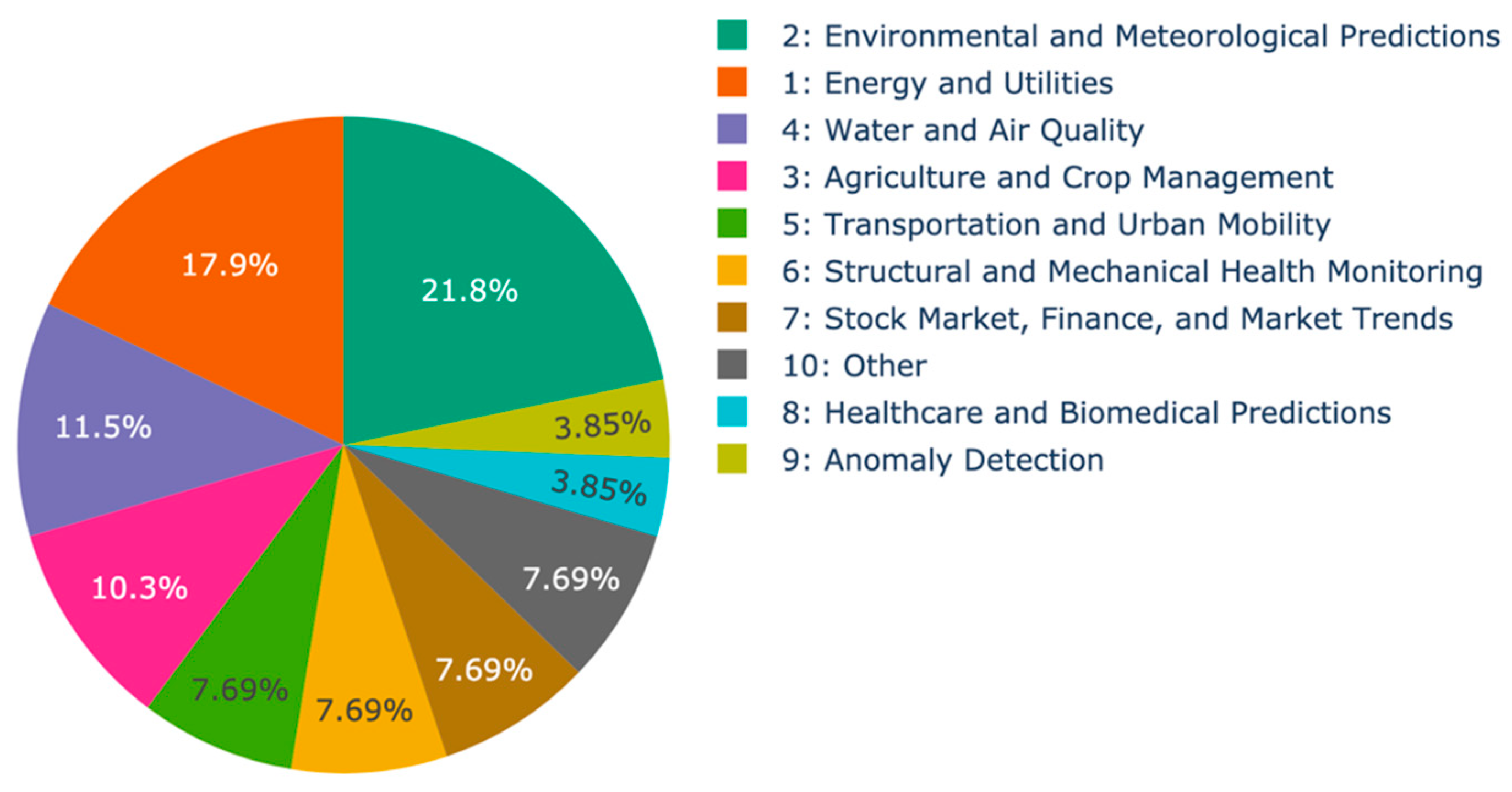
• TBML Models: these outperform in tasks related to energy and utilities, transportation and urban mobility, anomaly detection, and miscellaneous applications;
• DL Models: these outperform in tasks related to environmental and meteorological predictions, structural and mechanical health monitoring, and financial/market trend forecasting;
• SPTB Models: these outperform in tasks related to transportation and miscellaneous applications, while RNN models dominate in environmental, healthcare, and finance-related tasks;
• RNN Models: these outperform in tasks related to Environmental and Meteorological Predictions, Water and Air Quality, Structural and Mechanical Health Monitoring, Stock Market/Finance/Market Trends, and Healthcare and Biomedical Predictions.

It is important to note that the dataset includes relatively small representations for some categories (ranging from 3.85% to 21.8% of the total papers). As a result, the findings presented here do not present definitive evidence that any one type of model is dominant within a given domain. Instead, they highlight interesting patterns and trends that merit further investigation and validation with larger datasets. However, there are several explanations that can account for the performance differential between models.

TBML models excel in areas with tabular, noisy, missing, and categorical data, making them especially suitable for the domain of utilities, transportation, urban mobility, and anomaly detection, which often involve structured, tabular datasets that may have many sparse features. TBML models are especially equipped for anomaly detection as they are able to use the tree splitting criteria to capture feature interactions without needing much explicit feature engineering. Similarly, SPTB algorithms excel in transportation and miscellaneous applications as they are optimized for speed and do not require extensive feature engineering, making them compatible for a wide array of miscellaneous applications. DL models outperform in environmental/meteorological predictions and mechanical health monitoring due to their ability to effectively capture unstructured and spatial–temporal patterns in the data. Additionally, DL models perform better in financial/market trend forecasting as these models are better able to handle lagged effects and temporal dependencies, with less feature engineering than TBML models. Specifically, RNN models excel in a wide range of tasks including Water and Air Quality, Environmental and Meteorological Predictions, Structural and Mechanical Health Monitoring, Stock Market/Finance/Market Trends, and Healthcare/Biomedical Predictions due to their unique ability to remember long-term dependencies. Patterns in these domains can span over days, weeks, and even months, and RNN models like LSTM are able to remember this information through memory gates without manual feature engineering.

Dataset Size: An analysis of the influence of the dataset size on the relative performance of machine learning models for time series prediction reveals some interesting trends. In ML tasks with the least amount of data, DL models perform comparably to TBML models overall. However, RNN models demonstrate a significant advantage over SPTB models. As the dataset size increases, DL models begin to show a slight edge over TBML models in the lower mid-sized range (2173–7800 samples), although the gap narrows in the upper mid-sized range (7800–35,712 samples). Across this range, RNN models continue to outperform SPTB models, though the margin diminishes, reflecting SPTB models’ growing robustness with increasing data. For larger datasets, TBML models gain a clear advantage over DL models, with their performance gap widening at the largest dataset range (206,573–11,275,200 samples). This trend demonstrates the scalability of TBML models, particularly SPTB models, in handling vast amounts of data.

The reason that DL and specifically RNN models are able to perform better on smaller datasets than TBML models is they are better able to handle latent representations if sequential inputs are strong, even on small amounts of data. TBML models lack inducitve bias for sequence learning and thus may stuggle on small datsets if not given the appropriately engineered sequential features. Conversely, TBML models, specifically SPTB models, outperform DL models on larger datsets as these algorithms are much more computationally efficient at dealing with large amounts of data while remaining robust to noise, missing values, or irrelevant features, allowing them to quickly capture complex patterns. DL models are comparatively computationally expensive, harder to optimize, and require careful preprocessing for noisy data. When DL models are not given adequate training resources or are not carefully optimized, they consistently underperform relative to their TBML counterparts. It is worth pointing out that these generalizations do not hold true in all circumstances. Study [15] showcases that DL models such as LSTM struggle with overfitting and generalization, especially on small datasets, due to the nature of the model architecture (there are a larger number of weights and deviation terms for learning). The easiest way to overcome this limitation is to expand the dataset, as shown in study [16]. If there are no other data available, then DL models may fall short to other TBML methods. Study [67] demonstrates that in situations where no extra data are available, gradient-boosted TBML techniques show a superior generalization ability and thus lead to higher prediction accuracy.

Temporal Resolution: This study examines the impact of time interval lengths on the performance of ML models for time series prediction. However, no consistent pattern or trend emerges across the time intervals. DL models perform better in some intervals, while TBML performs better in others. As such, there is no common thread that unites these results across all temporal resolutions studied. The reason for this may indicate that other aspects of the data composition or domain-specific tasks are more important and impactful on the model performance, leaving weak-to-nonexistent trends for temporal resolution differences.

Influence of Research Focus: A notable finding is the inherent bias in performance outcomes depending on the research focus of the paper. DL models significantly outperform TBML models in papers focused on DL techniques, and vice versa for TBML-focused research. This suggests that researchers may devote disproportionate attention to optimizing models aligned with their research focus while investing less effort in models they are using for comparative efforts. Readers should exercise caution when interpreting comparative results in such studies. In studies with no specific focus, TBML models slightly edge out DL models, providing an interesting case for their superior performance in “bias-free” papers. A potential explanation for this disparity is that the accuracy of DL models is more dependent on the regularization techniques used and hyperparmeter values chosen for testing compared to TBML models. When researchers are biased towards DL methods, they may spend more time on this aspect of model development compared to TBML model development, causing DL methods to perform better. If researchers do not invest enough time or effort in this area of model developemnt, then TBML models are more likely to outperform DL methods.

Computational Efficiency: One of the most impactful findings is the disparity in training times between TBML and DL models. TBML models were found to be, on average, two-to-four orders of magnitude faster than DL models. This makes TBML models particularly appealing for real-world applications where computational cost is a critical consideration.

Error Metrics: Popular error metrics for evaluating classification and regression tasks may provide valuable benchmarks for future research. These include classification metrics such as Recall, Precision, the F1 Score, and Accuracy, as well as Regression Metrics such as RMSE, MAE, MAPE, and MSE. Future research may benefit from aligning evaluation methods with these metrics to ensure comparability across studies. Additionally, researchers may want to consider using a novel weighted quality evaluation index (WQE) proposed by [89], which combines the four most popular regression metrics (RMSE, MAE, MAPE, and R²) into a single unified evaluation standard that more holistically captures the model performance.

Hyperparameter Optimization: A grid search is the most frequently used hyperparameter optimization method, but it is also the most computationally intensive. Bayesian Optimization offers a promising alternative, providing a similar performance with much lower computational demands. Methods such as OPTUNA’s automatic hyperparameter tuning software are also emerging as viable options for hyperparameter tuning.

Hybrid Models: This study finds strong evidence that combining models generally enhances their performance, as evidenced by numerous surveyed papers that implement hybrid approaches. These hybrid models consistently outperform individual models, with their performance often improving as more models are integrated. There are notable exceptions to this trend, discussed in Section 5.3.9, where individual models show a superior performance compared to hybrids. These individual model examples exclusively involve SPTB models, further underscoring the robust performance of these algorithms. When comparing hybrid configurations, the results reveal that combinations of SPTB models with RNN models yield particularly strong outcomes. Additionally, hybrid models incorporating either SPTB or RNN architectures with attention-based or CNN models also demonstrate notable performance improvements.

Anecdotal Findings: Beyond the quantitative analysis across all surveyed papers, several anecdotal observations offer additional insights:

• Feature Sensitivity: GBDT models are less affected by redundant or removed features, whereas the ANN performance drops significantly when redundant features are added [8];
• Feature Selection: When all features are provided, XGBoost consistently delivers the best performance. However, when variables are selected using forward selection, other DL models begin to outperform it. Interestingly, the XGBoost model utilizing all features outperforms the XGBoost model that uses only the forward-selected features [15];
• Domain-Specific Findings: LightGBM produces more accurate results for top research terms in emerging topics, even though it generally has higher errors than NN [37];
• Inference Time: One study reported inference times for their models. They compared an XGBoost model (0.001 s) with an LSTM model (0.311 s) and a Bi-LSTM model (1.45 s), finding XGBoost to be 311 times faster than Bi-LSTM and 1450 times faster than LSTM. This drastically faster inference time emphasizes its practicality in time-sensitive applications [74];
• Simulated vs. Real-World Data: LightGBM matches the neural network performance on simulated data, but outperforms on real-world datasets [51];
• Time-Series Image Data: CNN models excel in prediction tasks involving time-series image data [3,23,44].

6. M5 and M6 Forecasting Competitions

Besides looking at research papers that focus on using ML models for real world applications in time series prediction, competitions that challenge teams to create models for a common dataset provide valuable insights into the comparative performance of machine learning methods. These contests enable direct comparisons under the same controlled conditions. Among such competitions, the M Forecasting Competitions stand out as the most prominent, well-structured, and well-funded. This section focuses on the two most recent iterations: the M5 and M6 Forecasting Competitions.

6.1. M5 Forecasting Competition

The M5 Forecasting Competition, held in 2020, focused on predicting retail sales using real-world data which consisted of 42,840 time series of Walmart unit sales. The competition had two components: the Accuracy Competition and the Uncertainty Competition, each with a prize pool of USD 50,000. These incentives attracted thousands of participants, creating a large dataset for analysis.

6.1.1. M5 Accuracy Competition

The M5 Accuracy Competition [90] tasked participants with providing the most accurate point forecasts, evaluated using a Weighted Root Mean Squared Scaled Error (WRMSSE) metric. A total of 5507 teams from 101 countries participated, with LightGBM emerging as the dominant model among the top 50 best performing teams. Brief insights from the top five models include the following:

• First Place: combined recursive and non-recursive LightGBM models to create 220 models, where the average of 6 models was used to forecast the series, each exploiting a different learning approach and training set;
• Second Place: created 50 LightGBM models, 5 for each of the 10 stores, utilizing a DL neural network to adjust multipliers based on historical sales data for each store;
• Third Place: employed 43 recursive neural networks (LSTMs) incorporating over 100 features;
• Fourth Place: created 40 non-recursive LightGBM models;
• Fifth Place: utilized seven recursive LightGBM models.

Nearly all of the top 50 submissions applied the last four 28-day windows of data for cross-validation to fine-tune the hyperparameters. Many top-performing teams, including 1st and 3rd place, used exogenous features like special days and zero-sales periods in their models. The researchers of this challenge concluded that the competition reinforced the value of model combination, cross-learning, and cross-validation. New findings included the superior performance of the LightGBM model compared to all others, as well as the importance of exogenous/explanatory variables used for forecasting.

6.1.2. M5 Uncertainty Competition

The Uncertainty competition [91] tasked participants with forecasting the distribution of realized values, requiring predictions of nine quantiles (0.005, 0.025, 0.165, 0.250, 0.500, 0.750, 0.835, 0.975, and 0.995). The Weighted Scaled Pinball Loss function was used to evaluate the performance. Although this competition was less popular, attracting 892 teams, the reliance on LightGBM models remained consistent, with four of the top five submissions incorporating it in their frameworks. Brief insights from the top five models include the following:

• First Place: utilized 126 LightGBM models, one for each quantile and aggregation level;
• Second Place: combined recursive LightGBM models, statistical methods, and simple time series forecasting techniques;
• Third Place: employed a hybrid approach integrating LightGBM and neural networks;
• Fourth Place: used two LSTM-based neural networks;
• Fifth Place: implemented 280 LightGBM models in a comprehensive ensemble.

A Monte Carlo simulation, used by the sixth-place team, was the only top-50 method not involving LightGBM, XGBoost, or neural networks. The findings from the Uncertainty competition mirrored those of the Accuracy competition, reaffirming the dominance of LightGBM and the importance of model combination. A notable observation was the stark contrast in participant expertise: while the Accuracy competition was won by an undergraduate student with limited knowledge in the domain of retail sales, the Uncertainty competition was dominated by Kaggle masters and grandmasters with strong statistical backgrounds.

6.2. M6 Forecasting Competition

The M6 forecasting competition from 2022 to 2023 [92] marked a significant evolution in the M series. With a prize pool of USD 300,000, it attracted 226 teams to participate. The challenge revolved around creating investment portfolios using real-time data from 50 U.S. stocks and 50 exchange-traded funds (ETFs). Unlike prior iterations, the M6 competition emphasized both forecasting and investment decision making, awarding prizes for the forecasting accuracy, investment performance, and overall performance. Participants were given flexibility in their data sources and methodologies. While organizers provided an optional dataset of adjusted closing values, teams could choose their own data, frequency, and supporting information, such as economic indicators or news. The competition spanned 12 months, with teams submitting monthly forecasts and investment strategies for the subsequent 20 trading days.

The winners in forecasting, investment, and the combined “duathlon” category all used distinct methods. The top forecasting model used a Bayesian dynamic factor model. The best-performing investment model relied on AutoTS, an open-source library for probabilistic time series forecasting. The duathlon champion employed a meta-learning model using NNs, which ranked fourth in forecasting. Notably, an XGBoost-based approach secured second place in both forecasting and the duathlon. Interestingly, the team that won the investment challenge placed 92nd in forecasting, and the second-place investment team, which used a type of exponential smoothing model (ATA), ranked 110th in forecasting. In fact, the researchers found zero correlation between forecasting and the investment performance, emphasizing that a team’s ability to accurately predict a stock’s future price was not the driving factor in creating the most profitable investment portfolio.

The researchers were not surprised that the best performing methods included both conventional econometric time series methods as well as sophisticated machine learning methods because of the unique challenges present in financial forecasting including external factors, seasonality, stochastic trends, etc. The key takeaway from the M6 competition is that the choice of data and their usage are as critical as the forecasting techniques themselves in achieving superior results.

6.3. Takeaways from M5 and M6 Forecasting Competitions

One of the most notable takeaways from the M5 competition was the dominance of LightGBM. Its ease of use allowed even relatively inexperienced participants to excel, as evidenced by the first-place finisher in the M5 Accuracy Competition, an undergraduate student. Most top-performing teams relied on ensembles of LightGBM models, leveraging its efficiency in handling large datasets. The results of the M5 competition also emphasized the importance of combining multiple models. Most top teams utilized ensembles, often containing hundreds of individual models, to enhance the accuracy of their predictions. Across both the M5 and M6 competitions, cross-validation (CV) and hyperparameter tuning emerged as indispensable components of successful forecasting methodologies. All top-performing teams employed thorough CV to optimize their models.

One critical takeaway from the M6 competition was the importance of the data quality, feature engineering, and the inclusion of exogenous variables. Unlike the M5 competition, where all participants worked with a standardized dataset, M6 participants were responsible for sourcing their own data. The complexity of this competition, including the unique challenges in the financial domain, also resulted in the number of participating teams to decrease to less than 4% of the M5 competition’s turnout (despite a substantial increase in incentives). The results of the competition showed no clear consensus on the best-performing methodology and suggest that the importance of the data quality and strong feature engineering, including the exogenous variables chosen, often outweighs the importance in the choice of the prediction model itself.

7. Conclusions

This survey of machine learning methods for time series prediction illuminates several key strategies for approaching time series forecasting tasks.

Table 3. Summary table of best-performing models for each data characteristic.

Dataset Size	Best-Performing Model Class	Best-Performing Model Subclass
Small (0–2173)	TBML/DL	RNN
Small/Medium (2173–7800)	DL	SPTB/RNN
Medium (7800–35,712)	TBML	RNN
Medium/Large (35,712)	TBML	SPTB/RNN
Large (206,573-11,275,200)	TBML	SPTB
Task Category	Best-Performing Model Class	Best-Performing Model Subclass
Energy and Utilities	TBML	SPTB
Environmental and Meteorological	DL	RNN
Agriculture and Crop Management	TBML	SPTB
Water and Air Quality	TBML	RNN
Transportation and Urban Mobility	TBML	SPTB
Structural and Mechanical Health Monitoring	DL	RNN
Stock Market, Finance, and Market Trends	DL	RNN
Healthcare and Biomedical Predictions	TBML	RNN
Anomaly Detection	TBML	SPTB/RNN
Other	TBML	SPTB
Time Interval	Best-Performing Model Class	Best-Performing Model Subclass
1 min	TBML/DL	RNN
5, 10 min	DL	RNN
15, 30 min	DL	RNN
1, 4 h	TBML	SPTB
1 day	TBML/DL	RNN
1 week, 8 day, 15 day, 16 day	TBML	SPTB
1 month	DL	RNN
Computational Efficiency	Best-Performing Model Class	Best-Performing Model Subclass
Training Time	TBML	SPTB
Inference time	TBML	SPTB

provides a visual overview of the best-performing models from the research in this study based on the data characteristics chosen. Based on these findings, the following approach is recommended for researchers and practitioners tackling time series prediction problems.

First and foremost, the domain and data play a pivotal role in determining the success of a forecasting model. Careful domain analysis to identify the most impactful data sources, coupled with meticulous feature engineering to extract and construct relevant features, should be the initial focus. The importance of high-quality data and strong exogenous features cannot be overstated, as evidenced by both the findings of this study and the results of recent forecasting competitions. Investing significant effort in this phase is likely to yield the greatest dividends in the predictive performance. Once the data are prepared, starting with a Tree-Based Machine Learning (TBML) model like LightGBM—or CatBoost for datasets with a high proportion of categorical features—is a logical choice. These gradient-boosting methods offer several advantages: they are computationally efficient, require less feature selection, and have demonstrated a competitive or superior performance compared to deep learning approaches in various settings. Such models serve as a low-cost baseline for experimentation and iterative improvement.

The model evaluation should be guided by task-specific metrics. For regression problems, metrics such as the Mean Absolute Error (MAE) or Root Mean Squared Error (RMSE) are appropriate, while classification tasks should use Recall, Precision, the F1 Score, and Accuracy. Hyperparameter tuning is another critical component of the modeling process. If prior knowledge exists about potential hyperparameter values, a grid search can be employed for systematic exploration. Otherwise, techniques like Bayesian Optimization or libraries such as OPTUNA are recommended for their ability to efficiently explore large parameter spaces and identify optimal configurations. If the initial model fails to meet the desired performance standards or further enhancements are required, Recurrent Neural Networks (RNNs), such as LSTMs or GRUs, are a logical next step. When building a deep learning model, it is crucial to carefully select and preprocess features to optimize the model’s performance and ensure it delivers the best results. As with earlier stages, hyperparameter tuning should be employed to maximize the performance. Finally, combining models—such as the initial TBML model with a deep learning model—can often yield superior results. Ensemble methods leverage the strengths of multiple methodologies, capturing diverse patterns and mitigating weaknesses inherent to any single approach, as demonstrated in this study.

In conclusion, effective time series prediction is a combination of domain knowledge, data quality, rigorous preprocessing, and the strategic application of the best machine learning methodologies. Starting with scalable and interpretable TBML models, fine-tuning their parameters, and iteratively incorporating advanced techniques like DL provides an efficient framework for tackling time series forecasting challenges. By following this approach, researchers and practitioners can maximize the predictive accuracy while optimizing computational costs in a variety of domains.

8. Future Work

There are several areas of future work that researchers could focus on to expand the insights of this paper, especially in areas of growing importance in the field of DL. One of these areas that was briefly touched upon in this paper and that warrants future research is Transformer-based architectures. The initial research indicates that transformers excel in long-range dependency modeling and thus perform well in the reviewed papers [28,33,70,74,77], showcasing a performance on par with the best-performing models in the literature. As there are only five research papers included in this study, future research should investigate the validity of this by exploring more recent papers where transformer models are being applied to time series applications. One of the biggest challenges that faces attention-based architectures is their significant computational cost. An interesting area to explore in addressing this is pre-trained transformer models [93]. These models can be pre-trained on large collections of unrelated time series data, enabling the improved performance of training on datasets across domains.

Other areas that future researchers could focus on include Diffusion Models and Neural Ordinary Differential Equation Models. Differential Equation Models have shown success in text, image, and video applications and recently have started to be applied to time series forecasting use cases (for a comprehensive review of diffusion models for time series applications, see [94]). Future research should focus on combatting the exceptionally high computational cost associated with the Diffusion Models applied to time series applications while maintaining high accuracy. Similarly, Neural Ordinary Differential Equations offer a modeling framework that provides a principled approach for forecasting continuous time series data by combining neural networks with the mathematics of differential equations (for a comprehensive review of Neural Ordinary Differential Equations for time series applications, see [95]). Neural Ordinary Differential Equations involve solving differential equations at a training and inference time which can be computationally very expensive. Future research in this field should focus on reducing these computational demands by developing more efficient solvers to increase the practicality of this DL architecture for time series forecasting applications.

References

1. Lim, B.; Zohren, S. Time-series forecasting with deep learning: A survey. Philos. Trans. R. Soc. A Math. Phys. Eng. Sci. 2021, 379, 20200209. [Google Scholar] [CrossRef]
2. Liu, Z.; Zhu, Z.; Gao, J.; Xu, C. Forecast Methods for Time Series Data: A Survey. IEEE Access 2021, 9, 91896–91912. [Google Scholar] [CrossRef]
3. Zhong, L.; Hu, L.; Zhou, H. Deep learning based multi-temporal crop classification. Remote Sens. Environ. 2019, 221, 430–443. [Google Scholar] [CrossRef]
4. Ke, J.; Zheng, H.; Yang, H.; Chen, X. Short-term forecasting of passenger demand under on-demand ride services: A spatio-temporal deep learning approach. Transp. Res. Part C Emerg. Technol. 2017, 85, 591–608. [Google Scholar] [CrossRef]
5. Ju, Y.; Sun, G.; Chen, Q.; Zhang, M.; Zhu, H.; Rehman, M.U. A Model Combining Convolutional Neural Network and LightGBM Algorithm for Ultra-Short-Term Wind Power Forecasting. IEEE Access 2019, 7, 28309–28318. [Google Scholar] [CrossRef]
6. Rafi, S.H.; Nahid Al, M.; Deeba, S.R.; Hossain, E. A Short-Term Load Forecasting Method Using Integrated CNN and LSTM Network. IEEE Access 2021, 9, 32436–32448. [Google Scholar] [CrossRef]
7. Galicia, A.; Talavera-Llames, R.; Troncoso, A.; Koprinska, I.; Martínez-Álvarez, F. Multi-step forecasting for big data time series based on ensemble learning. Knowl. -Based Syst. 2019, 163, 830–841. [Google Scholar] [CrossRef]
8. Bagherzadeh, F.; Mehrani, M.-J.; Basirifard, M.; Roostaei, J. Comparative study on total nitrogen prediction in wastewater treatment plant and effect of various feature selection methods on machine learning algorithms performance. J. Water Process Eng. 2021, 41, 102033. [Google Scholar] [CrossRef]
9. Kang, Y.; Ozdogan, M.; Zhu, X.; Ye, Z.; Hain, C.; Anderson, M. Comparative assessment of environmental variables and machine learning algorithms for maize yield prediction in the US Midwest. Environ. Res. Lett. 2020, 15, 064005. [Google Scholar] [CrossRef]
10. Chakraborty, D.; Elzarka, H. Advanced machine learning techniques for building performance simulation: A comparative analysis. J. Build. Perform. Simul. 2019, 12, 193–207. [Google Scholar] [CrossRef]
11. Zheng, J.; Zhang, H.; Dai, Y.; Wang, B.; Zheng, T.; Liao, Q.; Liang, Y.; Zhang, F.; Song, X. Time series prediction for output of multi-region solar power plants. Appl. Energy 2020, 257, 114001. [Google Scholar] [CrossRef]
12. Zhang, Y.; Li, C.; Jiang, Y.; Sun, L.; Zhao, R.; Yan, K.; Wang, W. Accurate prediction of water quality in urban drainage network with integrated EMD-LSTM model. J. Clean. Prod. 2022, 354, 131724. [Google Scholar] [CrossRef]
13. Mazzia, V.; Khaliq, A.; Chiaberge, M. Improvement in Land Cover and Crop Classification based on Temporal Features Learning from Sentinel-2 Data Using Recurrent-Convolutional Neural Network (R-CNN). Appl. Sci. 2020, 10, 238. [Google Scholar] [CrossRef]
14. Barrera-Animas, A.Y.; Oyedele, L.O.; Bilal, M.; Akinosho, T.D.; Delgado, J.M.D.; Akanbi, L.A. Rainfall prediction: A comparative analysis of modern machine learning algorithms for time-series forecasting. Mach. Learn. Appl. 2022, 7, 100204. [Google Scholar] [CrossRef]
15. Shin, Y.; Kim, T.; Hong, S.; Lee, S.; Lee, E.; Hong, S.; Lee, C.; Kim, T.; Park, M.S.; Park, J.; et al. Prediction of Chlorophyll-a Concentrations in the Nakdong River Using Machine Learning Methods. Water 2020, 12, 1822. [Google Scholar] [CrossRef]
16. Luo, J.; Zhang, Z.; Fu, Y.; Rao, F. Time series prediction of COVID-19 transmission in America using LSTM and XGBoost algorithms. Results Phys. 2021, 27, 104462. [Google Scholar] [CrossRef]
17. Gong, M.; Bai, Y.; Qin, J.; Wang, J.; Yang, P.; Wang, S. Gradient boosting machine for predicting return temperature of district heating system: A case study for residential buildings in Tianjin. J. Build. Eng. 2020, 27, 100950. [Google Scholar] [CrossRef]
18. Wang, Z.; Hong, T.; Li, H.; Ann Piette, M. Predicting city-scale daily electricity consumption using data-driven models. Adv. Appl. Energy 2021, 2, 100025. [Google Scholar] [CrossRef]
19. Yang, Y.; Heppenstall, A.; Turner, A.; Comber, A. Using graph structural information about flows to enhance short-term demand prediction in bike-sharing systems. Comput. Environ. Urban Syst. 2020, 83, 101521. [Google Scholar] [CrossRef]
20. Wei, Z.; Zhang, T.; Yue, B.; Ding, Y.; Xiao, R.; Wang, R.; Zhai, X. Prediction of residential district heating load based on machine learning: A case study. Energy 2021, 231, 120950. [Google Scholar] [CrossRef]
21. Zahoor Ali, K.; Muhammad, A.; Javaid, N.; Malik, N.S.; Shafiq, M.; Choi, J.-G. Electricity Theft Detection Using Supervised Learning Techniques on Smart Meter Data. Sustainability 2020, 12, 8023. [Google Scholar] [CrossRef]
22. Hussein, E.A.; Thron, C.; Ghaziasgar, M.; Bagula, A.; Vaccari, M. Groundwater Prediction Using Machine-Learning Tools. Algorithms 2020, 13, 300. [Google Scholar] [CrossRef]
23. Su, H.; Wang, A.; Zhang, T.; Qin, T.; Du, X.; Yan, X.-H. Super-resolution of subsurface temperature field from remote sensing observations based on machine learning. Int. J. Appl. Earth Obs. Geoinf. 2021, 102, 102440. [Google Scholar] [CrossRef]
24. Kumar, V.; Kedam, N.; Sharma, K.V.; Mehta, D.J.; Caloiero, T. Advanced Machine Learning Techniques to Improve Hydrological Prediction: A Comparative Analysis of Streamflow Prediction Models. Water 2023, 15, 2527. [Google Scholar] [CrossRef]
25. Jing, Y.; Hu, H.; Guo, S.; Wang, X.; Chen, F. Short-Term Prediction of Urban Rail Transit Passenger Flow in External Passenger Transport Hub Based on LSTM-LGB-DRS. IEEE Trans. Intell. Transp. Syst. 2021, 22, 4611–4621. [Google Scholar] [CrossRef]
26. Li, Y.; Bao, T.; Gao, Z.; Shu, X.; Zhang, K.; Xie, L.; Zhang, Z. A new dam structural response estimation paradigm powered by deep learning and transfer learning techniques. Struct. Health Monit. 2022, 21, 770–787. [Google Scholar] [CrossRef]
27. Yu, G.; Zhang, S.; Hu, M.; Wang, Y.K. Prediction of Highway Tunnel Pavement Performance Based on Digital Twin and Multiple Time Series Stacking. Adv. Civ. Eng. 2020, 2020, 8824135. [Google Scholar] [CrossRef]
28. Torres, J.F.; Martínez-Álvarez, F.; Troncoso, A. A deep LSTM network for the Spanish electricity consumption forecasting. Neural Comput. Appl. 2022, 34, 10533–10545. [Google Scholar] [CrossRef]
29. Ge, Y.; Wang, Q.; Wang, L.; Wu, H.; Peng, C.; Wang, J.; Xu, Y.; Xiong, G.; Zhang, Y.; Yi, Y. Predicting post-stroke pneumonia using deep neural network approaches. Int. J. Med. Inform. 2019, 132, 103986. [Google Scholar] [CrossRef]
30. Li, G.; Zhang, A.; Zhang, Q.; Wu, D.; Zhan, C. Pearson Correlation Coefficient-Based Performance Enhancement of Broad Learning System for Stock Price Prediction. IEEE Trans. Circuits Syst. II Express Briefs 2022, 69, 2413–2417. [Google Scholar] [CrossRef]
31. Sundararajan, K.; Garg, L.; Srinivasan, K.; Ali Kashif, B.; Jayakumar, K.; Ganapathy, G.P.; Senthil Kumaran, S.; Meena, T. A Contemporary Review on Drought Modeling Using Machine Learning Approaches. Comput. Model. Eng. Sci. 2021, 128, 447–487. [Google Scholar] [CrossRef]
32. Wu, W.; Chen, J.; Yang, Z.; Tindall, M.L. A Cross-Sectional Machine Learning Approach for Hedge Fund Return Prediction and Selection. Manag. Sci. 2021, 67, 4577–4601. [Google Scholar] [CrossRef]
33. López Santos, M.; García-Santiago, X.; Echevarría Camarero, F.; Blázquez Gil, G.; Carrasco Ortega, P. Application of Temporal Fusion Transformer for Day-Ahead PV Power Forecasting. Energies 2022, 15, 5232. [Google Scholar] [CrossRef]
34. Shangguan, Q.; Fu, T.; Wang, J.; Fang, S.e.; Fu, L. A proactive lane-changing risk prediction framework considering driving intention recognition and different lane-changing patterns. Accid. Anal. Prev. 2022, 164, 106500. [Google Scholar] [CrossRef] [PubMed]
35. Prodhan, F.A.; Zhang, J.; Yao, F.; Shi, L.; Pangali Sharma, T.P.; Zhang, D.; Cao, D.; Zheng, M.; Ahmed, N.; Mohana, H.P. Deep Learning for Monitoring Agricultural Drought in South Asia Using Remote Sensing Data. Remote Sens. 2021, 13, 1715. [Google Scholar] [CrossRef]
36. Khan, P.W.; Byun, Y.C.; Park, N.; Waqas Khan, P.; Byun, Y.-C.; Lee, S.-J.; Park, N. Machine Learning Based Hybrid System for Imputation and Efficient Energy Demand Forecasting. Energies 2020, 13, 2681. [Google Scholar] [CrossRef]
37. Liang, Z.; Mao, J.; Lu, K.; Ba, Z.; Li, G. Combining deep neural network and bibliometric indicator for emerging research topic prediction. Inf. Process. Manag. 2021, 58, 102611. [Google Scholar] [CrossRef]
38. Cui, Z.; Qing, X.; Chai, H.; Yang, S.; Zhu, Y.; Wang, F. Real-time rainfall-runoff prediction using light gradient boosting machine coupled with singular spectrum analysis. J. Hydrol. 2021, 603, 127124. [Google Scholar] [CrossRef]
39. Shen, M.; Luo, J.; Cao, Z.; Xue, K.; Qi, T.; Ma, J.; Liu, D.; Song, K.; Feng, L.; Duan, H. Random forest: An optimal chlorophyll-a algorithm for optically complex inland water suffering atmospheric correction uncertainties. J. Hydrol. 2022, 615, 128685. [Google Scholar] [CrossRef]
40. Teinemaa, I.; Dumas, M.; Leontjeva, A.; Maggi, F.M. Temporal stability in predictive process monitoring. Data Min. Knowl. Discov. 2018, 32, 1306–1338. [Google Scholar] [CrossRef]
41. Kwon, D.H.; Kim, J.B.; Han, Y.H. Time Series Classification of Cryptocurrency Price Trend Based on a Recurrent LSTM Neural Network. J. Inf. Process. Syst. 2019, 15, 694–706. [Google Scholar] [CrossRef]
42. Geng, L.; Che, T.; Ma, M.; Tan, J.; Wang, H. Corn Biomass Estimation by Integrating Remote Sensing and Long-Term Observation Data Based on Machine Learning Techniques. Remote Sens. 2021, 13, 2352. [Google Scholar] [CrossRef]
43. Ngarambe, J.; Irakoze, A.; Yun, G.Y.; Kim, G. Comparative Performance of Machine Learning Algorithms in the Prediction of Indoor Daylight Illuminances. Sustainability 2020, 12, 4471. [Google Scholar] [CrossRef]
44. Seydi, S.T.; Amani, M.; Ghorbanian, A. A Dual Attention Convolutional Neural Network for Crop Classification Using Time-Series Sentinel-2 Imagery. Remote Sens. 2022, 14, 498. [Google Scholar] [CrossRef]
45. Pan, S.; Yang, B.; Wang, S.; Guo, Z.; Wang, L.; Liu, J.; Wu, S. Oil well production prediction based on CNN-LSTM model with self-attention mechanism. Energy 2023, 284, 128701. [Google Scholar] [CrossRef]
46. Paudel, D.; de Wit, A.; Boogaard, H.; Marcos, D.; Osinga, S.; Athanasiadis, I.N. Interpretability of deep learning models for crop yield forecasting. Comput. Electron. Agric. 2023, 206, 107663. [Google Scholar] [CrossRef]
47. Ghimire, S.; Nguyen-Huy, T.; Al-Musaylh, M.S.; Deo, R.C.; Casillas-Pérez, D.; Salcedo-Sanz, S. A novel approach based on integration of convolutional neural networks and echo state network for daily electricity demand prediction. Energy 2023, 275, 127430. [Google Scholar] [CrossRef]
48. Zhu, X.; Guo, H.; Huang, J.J.; Tian, S.; Zhang, Z. A hybrid decomposition and Machine learning model for forecasting Chlorophyll-a and total nitrogen concentration in coastal waters. J. Hydrol. 2023, 619, 129207. [Google Scholar] [CrossRef]
49. Ravichandran, T.; Gavahi, K.; Ponnambalam, K.; Burtea, V.; Mousavi, S.J. Ensemble-based machine learning approach for improved leak detection in water mains. J. Hydroinform. 2021, 23, 307–323. [Google Scholar] [CrossRef]
50. Li, L.; Dai, S.; Cao, Z.; Hong, J.; Jiang, S.; Yang, K. Using improved gradient-boosted decision tree algorithm based on Kalman filter (GBDT-KF) in time series prediction. J. Supercomput. 2020, 76, 6887–6900. [Google Scholar] [CrossRef]
51. Hewamalage, H.; Bergmeir, C.; Bandara, K. Global models for time series forecasting: A Simulation study. Pattern Recognit. 2022, 124, 108441. [Google Scholar] [CrossRef]
52. Li, Y.; Yang, C.; Sun, Y. Dynamic Time Features Expanding and Extracting Method for Prediction Model of Sintering Process Quality Index. IEEE Trans. Ind. Inform. 2022, 18, 1737–1745. [Google Scholar] [CrossRef]
53. Srivastava, P.R.; Eachempati, P. Deep Neural Network and Time Series Approach for Finance Systems: Predicting the Movement of the Indian Stock Market. J. Organ. End User Comput. 2021, 33, 204–226. [Google Scholar] [CrossRef]
54. Ting, P.Y.; Wada, T.; Chiu, Y.L.; Sun, M.T.; Sakai, K.; Ku, W.S.; Jeng, A.A.K.; Hwu, J.S. Freeway Travel Time Prediction Using Deep Hybrid Model—Taking Sun Yat-Sen Freeway as an Example. IEEE Trans. Veh. Technol. 2020, 69, 8257–8266. [Google Scholar] [CrossRef]
55. Shi, J.; He, G.; Liu, X. Anomaly Detection for Key Performance Indicators Through Machine Learning. In Proceedings of the 2018 International Conference on Network Infrastructure and Digital Content (IC-NIDC), Guiyang, China, 22–24 August 2018; pp. 1–5. [Google Scholar]
56. Joseph, R.V.; Mohanty, A.; Tyagi, S.; Mishra, S.; Satapathy, S.K.; Mohanty, S.N. A hybrid deep learning framework with CNN and Bi-directional LSTM for store item demand forecasting. Comput. Electr. Eng. 2022, 103, 108358. [Google Scholar] [CrossRef]
57. Safat, W.; Asghar, S.; Gillani, S.A. Empirical Analysis for Crime Prediction and Forecasting Using Machine Learning and Deep Learning Techniques. IEEE Access 2021, 9, 70080–70094. [Google Scholar] [CrossRef]
58. Qiu, H.; Luo, L.; Su, Z.; Zhou, L.; Wang, L.; Chen, Y. Machine learning approaches to predict peak demand days of cardiovascular admissions considering environmental exposure. BMC Med. Inform. Decis. Mak. 2020, 20, 83. [Google Scholar] [CrossRef]
59. Ribeiro, A.M.N.C.; do Carmo, P.R.X.; Endo, P.T.; Rosati, P.; Lynn, T. Short- and Very Short-Term Firm-Level Load Forecasting for Warehouses: A Comparison of Machine Learning and Deep Learning Models. Energies 2022, 15, 750. [Google Scholar] [CrossRef]
60. Priyadarshi, R.; Panigrahi, A.; Routroy, S.; Garg, G.K. Demand forecasting at retail stage for selected vegetables: A performance analysis. J. Model. Manag. 2019, 14, 1042–1063. [Google Scholar] [CrossRef]
61. Chen, H.; Guan, M.; Li, H. Air Quality Prediction Based on Integrated Dual LSTM Model. IEEE Access 2021, 9, 93285–93297. [Google Scholar] [CrossRef]
62. Ibañez, S.C.; Dajac, C.V.G.; Liponhay, M.P.; Legara, E.F.T.; Esteban, J.M.H.; Monterola, C.P. Forecasting Reservoir Water Levels Using Deep Neural Networks: A Case Study of Angat Dam in the Philippines. Water 2022, 14, 34. [Google Scholar] [CrossRef]
63. Pham Hoang, V.; Trinh Tan, D.; Tieu Khoi, M.; Hoang Vuong, P.; Tan Dat, T.; Khoi Mai, T.; Hoang Uyen, P.; The Bao, P. Stock-Price Forecasting Based on XGBoost and LSTM. Comput. Syst. Sci. Eng. 2022, 40, 237–246. [Google Scholar] [CrossRef]
64. Farsi, M. Application of ensemble RNN deep neural network to the fall detection through IoT environment. Alex. Eng. J. 2021, 60, 199–211. [Google Scholar] [CrossRef]
65. Nan, S.; Tu, R.; Li, T.; Sun, J.; Chen, H. From driving behavior to energy consumption: A novel method to predict the energy consumption of electric bus. Energy 2022, 261, 125188. [Google Scholar] [CrossRef]
66. Comert, G.; Khan, Z.; Rahman, M.; Chowdhury, M. Grey models for short-term queue length predictions for adaptive traffic signal control. Expert Syst. Appl. 2021, 185, 115618. [Google Scholar] [CrossRef]
67. Liu, S.; Zeng, A.; Lau, K.; Ren, C.; Chan, P.-w.; Ng, E. Predicting long-term monthly electricity demand under future climatic and socioeconomic changes using data-driven methods: A case study of Hong Kong. Sustain. Cities Soc. 2021, 70, 102936. [Google Scholar] [CrossRef]
68. Abdikan, S.; Sekertekin, A.; Narin, O.G.; Delen, A.; Balik Sanli, F. A comparative analysis of SLR, MLR, ANN, XGBoost and CNN for crop height estimation of sunflower using Sentinel-1 and Sentinel-2. Adv. Space Res. 2023, 71, 3045–3059. [Google Scholar] [CrossRef]
69. Phan, Q.T.; Wu, Y.K.; Phan, Q.D.; Lo, H.Y. A Novel Forecasting Model for Solar Power Generation by a Deep Learning Framework with Data Preprocessing and Postprocessing. IEEE Trans. Ind. Appl. 2023, 59, 220–231. [Google Scholar] [CrossRef]
70. Guan, S.; Wang, Y.; Liu, L.; Gao, J.; Xu, Z.; Kan, S. Ultra-short-term wind power prediction method based on FTI-VACA-XGB model. Expert Syst. Appl. 2024, 235, 121185. [Google Scholar] [CrossRef]
71. Wang, X.; Li, Y.; Qiao, Q.; Tavares, A.; Liang, Y. Water Quality Prediction Based on Machine Learning and Comprehensive Weighting Methods. Entropy 2023, 25, 1186. [Google Scholar] [CrossRef]
72. Li, Z.; Ma, E.; Lai, J.; Su, X. Tunnel deformation prediction during construction: An explainable hybrid model considering temporal and static factors. Comput. Struct. 2024, 294, 107276. [Google Scholar] [CrossRef]
73. Pavlov-Kagadejev, M.; Jovanovic, L.; Bacanin, N.; Deveci, M.; Zivkovic, M.; Tuba, M.; Strumberger, I.; Pedrycz, W. Optimizing long-short-term memory models via metaheuristics for decomposition aided wind energy generation forecasting. Artif. Intell. Rev. 2024, 57, 45. [Google Scholar] [CrossRef]
74. Zrira, N.; Kamal-Idrissi, A.; Farssi, R.; Khan, H.A. Time series prediction of sea surface temperature based on BiLSTM model with attention mechanism. J. Sea Res. 2024, 198, 102472. [Google Scholar] [CrossRef]
75. Mangukiya, N.K.; Sharma, A. Alternate pathway for regional flood frequency analysis in data-sparse region. J. Hydrol. 2024, 629, 130635. [Google Scholar] [CrossRef]
76. Zhang, L.; Wang, C.; Hu, W.; Wang, X.; Wang, H.; Sun, X.; Ren, W.; Feng, Y. Dynamic real-time forecasting technique for reclaimed water volumes in urban river environmental management. Environ. Res. 2024, 248, 118267. [Google Scholar] [CrossRef]
77. Zhao, Z.-h.; Wang, Q.; Shao, C.-s.; Chen, N.; Liu, X.-y.; Wang, G.-b. A state detection method of offshore wind turbines’ gearbox bearing based on the transformer and GRU. Meas. Sci. Technol. 2024, 35, 025903. [Google Scholar] [CrossRef]
78. Singh, R.B.; Patra, K.C.; Samantra, A.; Singh, R.B.; Patra, K.C.; Pradhan, B.; Samantra, A. HDTO-DeepAR: A novel hybrid approach to forecast surface water quality indicators. J. Environ. Manag. 2024, 352, 120091. [Google Scholar] [CrossRef]
79. Inbar, O.; Avisar, D. Enhancing wastewater treatment through artificial intelligence: A comprehensive study on nutrient removal and effluent quality prediction. J. Water Process Eng. 2024, 61, 105212. [Google Scholar] [CrossRef]
80. Oyucu, S.; Dümen, S.; Duru, İ.; Aksöz, A.; Biçer, E. Discharge Capacity Estimation for Li-Ion Batteries: A Comparative Study. Symmetry 2024, 16, 436. [Google Scholar] [CrossRef]
81. Saravanan, K.S.; Bhagavathiappan, V. Prediction of crop yield in India using machine learning and hybrid deep learning models. Acta Geophys. 2024, 72, 4613–4632. [Google Scholar] [CrossRef]
82. Chen, T.; Guestrin, C. XGBoost: A Scalable Tree Boosting System. In Proceedings of the 22nd ACM SIGKDD International Conference on Knowledge Discovery and Data Mining, San Francisco, CA, USA, 13–17 August 2016; pp. 785–794. [Google Scholar]
83. Ke, G.; Meng, Q.; Finley, T.; Wang, T.; Chen, W.; Ma, W.; Ye, Q.; Liu, T.-Y. LightGBM: A highly efficient gradient boosting decision tree. In Proceedings of the 31st International Conference on Neural Information Processing Systems, Long Beach, CA, USA, 4–9 December 2017; pp. 3149–3157. [Google Scholar]
84. Prokhorenkova, L.; Gusev, G.; Vorobev, A.; Dorogush, A.V.; Gulin, A. CatBoost: Unbiased boosting with categorical features. In Proceedings of the 32nd International Conference on Neural Information Processing Systems, Montréal, QC, Canada, 3–8 December 2018; pp. 6639–6649. [Google Scholar]
85. Svozil, D.; Kvasnicka, V.; Pospichal, J.í. Introduction to multi-layer feed-forward neural networks. Chemom. Intell. Lab. Syst. 1997, 39, 43–62. [Google Scholar] [CrossRef]
86. Gu, J.; Wang, Z.; Kuen, J.; Ma, L.; Shahroudy, A.; Shuai, B.; Liu, T.; Wang, X.; Wang, G.; Cai, J.; et al. Recent advances in convolutional neural networks. Pattern Recognit. 2018, 77, 354–377. [Google Scholar] [CrossRef]
87. Sherstinsky, A. Fundamentals of Recurrent Neural Network (RNN) and Long Short-Term Memory (LSTM) network. Phys. D Nonlinear Phenom. 2020, 404, 132306. [Google Scholar] [CrossRef]
88. Vaswani, A.; Shazeer, N.; Parmar, N.; Uszkoreit, J.; Jones, L.; Gomez, A.N.; Kaiser, Ł.; Polosukhin, I. Attention is all you need. In Proceedings of the 31st International Conference on Neural Information Processing Systems, Long Beach, CA, USA, 4–9 December 2017; pp. 6000–6010. [Google Scholar]
89. Yu, Z.; He, X.; Montillet, J.-P.; Wang, S.; Hu, S.; Sun, X.; Huang, J.; Ma, X. An improved ICEEMDAN-MPA-GRU model for GNSS height time series prediction with weighted quality evaluation index. GPS Solut. 2025, 29, 113. [Google Scholar] [CrossRef]
90. Makridakis, S.; Spiliotis, E.; Assimakopoulos, V. M5 accuracy competition: Results, findings, and conclusions. Int. J. Forecast. 2022, 38, 1346–1364. [Google Scholar] [CrossRef]
91. Makridakis, S.; Spiliotis, E.; Assimakopoulos, V.; Chen, Z.; Gaba, A.; Tsetlin, I.; Winkler, R.L. The M5 uncertainty competition: Results, findings and conclusions. Int. J. Forecast. 2022, 38, 1365–1385. [Google Scholar] [CrossRef]
92. Makridakis, S.; Spiliotis, E.; Hollyman, R.; Petropoulos, F.; Swanson, N.; Gaba, A. The M6 Forecasting Competition: Bridging the Gap Between Forecasting and Investment Decisions. Int. J. Forecast. 2024, in press. [Google Scholar] [CrossRef]
93. Woo, G.; Liu, C.; Kumar, A.; Xiong, C.; Savarese, S.; Sahoo, D. Unified training of universal time series forecasting transformers. In Proceedings of the 41st International Conference on Machine Learning, Vienna, Austria, 21–27 July 2024; p. 2178. [Google Scholar]
94. Lin, L.; Li, Z.; Li, R.; Li, X.; Gao, J. Diffusion models for time-series applications: A survey. Front. Inf. Technol. Electron. Eng. 2024, 25, 19–41. [Google Scholar] [CrossRef]
95. Oh, Y.; Kam, S.; Lee, J.; Lim, D.-Y.; Kim, S.; Bui, A. Comprehensive Review of Neural Differential Equations for Time Series Analysis. arXiv 2025. [Google Scholar] [CrossRef]
Figure 1. Architectural differences between RF and GBDT, where attributes unique to RF are labeled in green and those specific to GBDT are labeled in blue. Solid arrows represent connections consistent across all architectures, and dashed arrows represent deviations for specific architectures.
Applsci 15 05957 g001
Figure 2. Architecture of an FFNN, including the modifications needed to transform it into a CNN (labeled in orange) or an RNN (labeled in red). Solid arrows represent connections consistent across all architectures, and dashed arrows represent deviations for specific architectures.
Applsci 15 05957 g002
Figure 3. FPA and WRA score distribution for each class, including the comparative performance (%) between the two classes.
Applsci 15 05957 g003
Figure 4. FPA and WRA scores for each model. The “Model Use” legend indicates the total number of comparisons for each model, with specific counts labeled above the bars.
Applsci 15 05957 g004
Figure 5. FPA scores for each model. The “Model Use” legend indicates the total number of comparisons for each model, with specific counts labeled above the bars.
Applsci 15 05957 g005
Figure 6. WRA scores for each model. The “Model Use” legend indicates the total number of comparisons for each model, with specific counts labeled above the bars.
Applsci 15 05957 g006
Figure 7. Distribution of time series prediction tasks by category, including group numbers and the percentage representation of each category.
Applsci 15 05957 g007
Figure 8. FPA scores for each model. Blue bars represent the overall model types, while orange bars highlight the best-performing model classes.
Applsci 15 05957 g008
Figure 9. WRA scores for each model. Blue bars represent the overall model types, while orange bars highlight the best-performing model classes.
Applsci 15 05957 g009
Figure 10. FPA percentage for each model based on dataset size. Blue bars represent the overall model types, while orange bars indicate the best-performing class of models. The dataset size range is exclusive on the lower bound and inclusive on the upper bound.
Applsci 15 05957 g010
Figure 11. WRA percentage for each model based on dataset size. Blue bars represent the overall model types, while orange bars indicate the best-performing class of models. The dataset size range is exclusive on the lower bound and inclusive on the upper bound.
Applsci 15 05957 g011
Figure 12. FPA score for each model based on time interval of data. Blue bars represent the overall model types, while orange bars indicate the best-performing class of models.
Applsci 15 05957 g012
Figure 13. WRA score for each model based on time interval of data. Blue bars represent the overall model types, while orange bars indicate the best-performing class of models.
Applsci 15 05957 g013
Figure 14. FPA score for each model class based on the focus of the paper.
Applsci 15 05957 g014
Figure 15. WRA score for each model class based on the focus of the paper.
Applsci 15 05957 g015
Figure 16. Percent of papers that use each error metric for classification tasks.
Applsci 15 05957 g016
Figure 17. Percent of papers that use each error metric for regression tasks.
Applsci 15 05957 g017
Figure 18. Usage for each hyperparameter optimization technique.
Applsci 15 05957 g018