Research on Multi-Objective Flexible Job Shop Scheduling Optimization Based on Improved Salp Swarm Algorithm in Rolling Production Mode

Abstract

To address the multi-objective flexible job shop scheduling problem in rolling production mode (FJSP-RPM), this study proposes a Multi Objective Improved of Salp Swarm Algorithm (MISSA) that simultaneously optimizes equipment utilization and total tardiness. The MISSA generates initial population through various heuristic strategies to improve the initial population quality. The exploitation capability of the algorithm is enhanced through the global crossover strategy and variety of local search strategies. In terms of improvement strategies, the MISSA (using all three strategies) outperforms other incomplete variant algorithms (using only two strategies) in three metrics: Generational Distance (GD), Inverted Generational Distance (IGD), and diversity metric, achieving superior results in 9 test cases, 8 test cases, and 4 test cases respectively. When compared with NSGA2, NSGA3, and SPEA2 algorithms, the MISSA demonstrates advantages in 8 test cases for GD, 8 test cases for IGD, and 7 test cases for the diversity metric. Additionally, the distribution of the obtained solution sets is significantly better than that of the comparative algorithms, which validats the effectiveness of the MISSA in solving FJSP-RPM.

1. Introduction

As a core challenge in manufacturing production planning, scheduling optimization for complex workshops significantly enhances enterprise productivity and reduces operational costs [1]. The flexible job shop scheduling problem (FJSP), an extension of the classical job shop scheduling problem (JSP), involves both process sequencing and machine allocation, rendering it NP-hard.

The approximate algorithm represented by metaheuristic optimization algorithm is a promising solution for FJSP. It can effectively mitigate the disadvantages of traditional exact algorithms such as high computational cost and difficulty in solving large-scale problems. Many studies have investigated this topic. Fei et al. [2] considered two objective functions, maximum completion time and carbon emissions. They used an improved chimpanzee optimization algorithm to solve the multi-objective green flexible workshop scheduling problem. By introducing improved mechanisms, such as dynamic convergence factor and variable neighborhood search, the exploitation capabilities of the algorithm were enhanced. In addition, the effectiveness of the algorithm in reducing carbon emissions in flexible workshops was verified through experiments. Han et al. [3] studied the integrated scheduling problem of FJSP and Automated Guided Vehicle (AGV) with the objective function of minimizing the maximum completion time. A new mixed integer linear programming model and dual population collaborative genetic algorithm was proposed. Xu et al. [4] proposed a hybrid algorithm combining quantum particle swarm optimization and variable neighborhood search to efficiently solve FJSP with the goal of maximum completion time. The stability and applicability of the algorithm were verified through testing on standard test cases and an industrial case. Huang et al. [5] used memetic algorithm to solve the problem of green type-2 fuzzy flexible workshop. Ensieh et al. [6] proposed a simulation optimization framework for solving stochastic flexible job shop scheduling problems in the semiconductor manufacturing industry. Philipp et al. [7] proposed a new solution algorithm based on quantum annealing, which combines the power of quantum annealing with classical techniques for calculating FJSP. Gong et al. [8] proposed an FJSP model with flexible discrete operation order, considering that some job operations in the real job process do not have any order constraints. They verified the effectiveness of the model through CPLEX (a mathematical programming solver developed by IBM). In summary, most current FJSP models aim to minimize the maximum completion time as their core objective. Metaheuristic optimization algorithms have demonstrated significant advantages in solving the FJSP.

However, traditional FJSP has two limitations. First, it is too idealistic. Current research is mostly based on the assumption of static scheduling, generating the global optimal solution at once. This deviates from the actual production of the enterprises. In actual machining operations, the scheduling workload is generally greater than the equipment capacity. New parts will be rolled into production at regular production cycles. The scheduling plan should be a periodic rolling adjustment. Therefore, this article describes a rolling production mode (defined in Section 3). The second limitation of traditional FJSP is that although FJSP has multiple scheduling objectives, current research mostly focuses on minimizing the maximum completion time as the core objective (without considering the delivery time of each workpiece). In the process of actual machining operations, each workpiece has an expected delivery date. On the one hand, enterprises need to avoid delays, and on the other hand, they hope to reduce equipment idle rates.

On this basis, this article proposes a flexible job shop scheduling model under the rolling production mode. The aim is to simultaneously maximize equipment utilization during the rolling production cycle and minimize total delay time to better meet the actual needs of enterprises. The Multi Objective Improved of Salp Swarm Algorithm (MISSA) is used to address this challenge. In order to extend the application of the SSA to workshop scheduling problems, a conversion strategy between real-coded vectors and integer-coded vectors is designed. In order to improve the quality of the initial population and accelerate the convergence speed of the algorithm, various heuristic strategies such as the maximum residual load rule and the shortest processing time rule are introduced. During the algorithm iteration process, corresponding global and local search strategies were designed for process sorting encoding and machine selection encoding to further enhance the exploitation capabilities of the improved algorithm. Finally, the feasibility of the improved strategy and the effectiveness of the improved algorithm were verified through comparative experiments.

2. Related Work

2.1. Rolling Production Mode

The emergence of the rolling production mode stems from enterprises’ dual needs to maximize equipment utilization and dynamically adapt to continuous orders. Firstly, manufacturers need to avoid idle equipment through continuous production task allocation. Secondly, in real-time order-receiving scenarios, new orders and corresponding workpieces continuously enter the production system. Unlike traditional FJSP, the rolling production mode does not create a scheduling plan for the entire production cycle at once. Instead, it divides the production plan into multiple cycles. At the end of each cycle, rescheduling is carried out based on the current production status, order demand, and resource availability. By continuously rolling adjustments and optimizing scheduling, the dynamic adaptability of the plan is maintained, and equipment utilization is fully maximized. Although some literature [9] mentions the rolling production mode, there is currently no authoritative study that formally defines this concept.

In order to improve equipment utilization, some studies have adopted a workpiece batching strategy to reduce the risk of equipment vacancy. For example, Pinar et al. [10] constructed a batch scheduling model under dual constraints of set time and transportation resources. Hajibabaei et al. [11] studied the scheduling problem of batch flow shop. A competitive and cooperative bird optimization algorithm was proposed in [12] for solving the batch scheduling problem in flexible job shops. Yu et al. [13] conducted research on batch processing and scheduling problems in mixed flow workshops. They minimize total job delays and improve machine utilization by determining the number and composition of batches. Ozturk et al. [14] proposed a branch and bound parallel batch scheduling algorithm that performs batch scheduling for jobs with different date attributes to improve device utilization. There are also methods that use rolling production planning to improve equipment utilization. For example, Huang et al. [9] proposed an improved genetic algorithm to solve the flexible job shop scheduling problem in rolling production mode. In summary, there is currently relatively little research on scenarios based on the rolling production mode.

2.2. Salp Swarm Algorithm

2.2.1. Basic Process of Salp Swarm Algorithm

In nature, salps form a chain like structure by connecting their heads and tails for foraging activities. As shown in Figure 1, the salp chain can be divided into two parts: leader and follower. Leader determines the direction of movement based on the location of the food source (in SSA, the food source represents the global optimal solution position found by the current population search) by guiding followers. Mirjalili [15] proposed an optimization algorithm for salps based on their predatory behavior. In SSA, the first salp on the chain serves as the leader, while the rest are followers. Unlike other swarm intelligence optimization algorithms, the behavior of the leader does not directly affect the movement of the entire group. Followers do not always completely follow the leader, but adjust their position based on the previous individual’s position, gradually forming a salp chain. Therefore, the influence of leaders on followers gradually weakens with distance, thus maintaining the diversity of the group. SSA ensures that the current optimal solution is not lost even if the population state deteriorates by saving it and assigning it to the food source variable. SSA only updates the leader’s position relative to the food source, as it represents the current optimal solution, and the leader continues to explore the surrounding area; followers improve local search performance by following behavior, reducing the risk of getting stuck in local optima.

The SSA is based on population evolution. During initialization, each individual of salps represents a candidate solution in the population. Each solution is randomly generated between the set upper bound $ub$ and lower bound $lb$. The initialization position of the salp population is:

$$X=\left[\begin{array}{c}\begin{array}{c}{X}^1\\ X^2\end{array}\\ ⋮\\ X^N\end{array}\right]=\left[\begin{array}{ccc}{x}_1^1& x_2^1& \begin{array}{cc}\dots & x_D^1\end{array}\\ x_1^2& x_2^2& \begin{array}{cc}\dots & x_D^2\end{array}\\ \begin{array}{c}⋮\\ x_1^N\end{array}& \begin{array}{c}⋮\\ x_2^N\end{array}& \begin{array}{cc}\begin{array}{c}\dots \\ \dots \end{array}& \begin{array}{c}⋮\\ x_D^N\end{array}\end{array}\end{array}\right]$$

(1)

Among them, N is the population size, D is the number of decision variables, and the algorithm initializes the position $X_j^i$ (i = 1, 2, …, N; j = 1, 2, …, D) of each individual salp by generating random numbers.

$$X_j^i\left(l\right)=rand\left(N,D\right)\left({ub}_j-{lb}_j\right)+{lb}_j$$

(2)

Among them, l is the current iteration number, and $X_j^i\left(l\right)$ is the position of the ith salp individual in the jth dimensional space. After obtaining the population of salps, calculate the fitness function value of each individual salp and sort them. Based on the sorting results, determine the food source, leader, and follower position. The positions of the leader and followers are represented by matrix $X_j^i$, and the formula for updating the position of the leader is:

$$X_j^i\left(l\right)=\left\{\begin{array}{c}{F}_j+c_1\left(\left({ub}_j-{lb}_j\right)c_2+{lb}_j\right), c_3\ge 0.5\\ F_j-c_1\left(\left({ub}_j-{lb}_j\right)c_2+{lb}_j\right), c_3\ge 0.5\end{array}\right.$$

(3)

Among them, $F_j$ represents the position of contemporary food sources in the jth dimensional space, and ${ub}_j, {lb}_j$ are the upper and lower limits of the jth dimensional search space. $c_2, c_3$ are random numbers evenly distributed between (0, 1), which play a role in adjusting the position in the leader update formula. $c_1$ is the correlation coefficient used to balance the exploitation of SSA, which decreases with the increase of iteration times to improve the development intensity in the later stage of algorithm iteration. The calculation formula for $c_1$ is:

$$c_1=2e^{-{\left({\displaystyle \frac{4t}{t_{max}}}\right)}^2}$$

(4)

Among them, t is the current iteration number of the algorithm, and $t_{max}$ is the maximum iteration number of the algorithm.

Followers follow the former in sequence to update their positions, and the position update formula is:

$$\begin{gathered} X_j^i\left(l\right)={\displaystyle \frac{1}{2}}\left(X_j^i\left(l-1\right)+X_j^{i-1}\left(l-1\right)\right) \\ i>1, l>1 \end{gathered}$$

(5)

Among them, $X_j^i\left(l\right)$ is the position of the contemporary salp follower, $X_j^i(l-1)$ and $X_j^{i-1}(l-1)$ are the positions of the previous generation salp followers i and i − 1 in the jth dimension space, respectively.

Due to the unclear location of the target food during the iteration process, it is necessary to calculate the fitness values of all individual salps for comparison, and set the position of the salp with the optimal fitness value as the current food source position. Finally, perform boundary processing on the updated individuals of salps to avoid crossing boundaries.

The basic workflow of the Salp Swarm Algorithm (SSA) can be summarized as follows:

• Step 1: Population Initialization

Randomly generate initial salp positions within the search space boundaries.

• Step 2: Fitness Evaluation

Calculate fitness values for all salps using the objective function.

• Step 3: Leader-Follower Division

Rank salps by fitness and split the population into two groups: Leaders for global exploration and followersfor local exploitation.

• Step 4: Leader Positions Updates (Global Search)

Update leader positions using Formula (3).

• Step 5: Follower Positions Updates (Local Search)

Adjust follower positions through chain-like movement using Formula (5).

• Step 6: Termination Check

Repeat steps 2–5 until reaching maximum iterations or convergence criteria.

2.2.2. Characteristics and Application Fields of SSA

SSA has the following advantages:

1.

Few parameters and easy to implement:

SSA only needs to adjust a few parameters such as population size and iteration times. The algorithm structure is simple and the implementation difficulty is low.

2.

Strong global search capability:

Through the leader follower chain structure, SSA can effectively explore the global optimal solution in the solution space.

3.

Highly self-organizing:

The group dynamic update mechanism does not require manual intervention and is suitable for complex optimization problems.

4.

Good compatibility with other algorithms:

Flexible integration with genetic algorithms [16], simulated annealing [17] and other algorithms to improve performance.

Due to the advantages of SSA, it has been applied to solve problems such as target classification [18], photovoltaic system optimization [19], feature extraction [20], image processing [21], and biomedical signal processing [22]. Some scholars have also applied SSA in the field of production scheduling, but it is not very common and is still in its infancy. Ewees et al. [23] proposed an improved SSA based on firefly algorithm to solve parallel machine scheduling problems. Zhao et al. [17] proposed an improved SSA based on Lévy flight integrated simulated annealing strategy to solve FJSP. Wei et al. [24] developed collaborative group search strategies and population diversity maintenance mechanisms to enhance the SSA optimization capabilities in addressing hybrid flow shop scheduling problems with setup operators.

The FJSP involves multiple coupled constraints such as process sequence and machine selection., Solving algorithms for FJSP must balance global and local optimization. Traditional Particle Swarm Optimization (PSO) tends to become trapped in local optima due to its single information-sharing mechanism, leading to degraded solution quality. Similarly, traditional Genetic Algorithms (GA) face challenges where crossover and mutation operations often compromise solution feasibility. When the fitting function in GA is poorly designed, the algorithm tends to favor locally superior individuals, causing rapid decline in population diversity and premature convergence to local optima. In contrast, the SSA inherently establishes a dynamic equilibrium mechanism through leader-guided global exploration and follower-driven local refinement, naturally balancing global and local search capabilities. In Reference [15], the SSA outperformed seven algorithms, including PSO and GA.

Existing research demonstrates the potential of SSA in solving workshop scheduling problems. However, SSA has the following limitations:

1.

The multi-objective FJSP is a discrete optimization problem. The position update formula for leaders and followers in SSA are designed for continuous optimization problems and cannot be directly applied to discrete problems. Among the studies mentioned above, only reference [24] mentioned a method to solve this problem, while others did not specifically address how to discretize the position formula in SSA. Reference [24] implemented discretization through threshold segmentation and probabilistic distribution sampling, which presets fixed threshold intervals to partition continuous spaces into non-overlapping discrete regions. Their method establishes probability distribution models for each interval, utilizing 8 parameters (with two assumed to follow normal distributions). However, this approach exhibits high dependency on manually configured thresholds and parameter sensitivity.

2.

When SSA approaches the potential optimal solution region, it requires excessive time to thoroughly search these areas. Weak exploitation capability leads to slow convergence speed. Regarding the solution of FJSP, current improvements in SSA have primarily focused on either modifying the position update formula [23], unilaterally strengthening local search capabilities [25], or singularly enhancing population diversity [24]. Existing approaches still lack systematic enhancements to holistically strengthen comprehensive exploitation capabilities.

This study aims to propose an improved SSA by adopting new mechanisms to address the aforementioned limitations of traditional SSA.

3. Problem Description and Model

The flexible job shop scheduling problem in rolling production mode (FJSP-RPM) can be defined as: a batch of workpieces need to be processed in the current scheduling cycle of the workshop, including n workpieces (J1, J2, ..., Jn), which need to be processed on a total of m machines (M1, M2, ..., Mm). The quantity of workpieces exceeds the equipment’s production capacity. $O_{ij}$ represents the jth process of workpiece i, ${\Omega }_{ij}$ represents the optional equipment set of the jth process of workpiece i, each process can be processed on any one of m devices with processing capacity, and equipment k can process more different workpieces process. Due to different performance characteristics of the equipment, the processing time for the same process varies among different devices. Each workpiece has a delivery deadline, where $d_i$ represents the delivery deadline for workpiece i. If the delivery time exceeds the delivery deadline, the manufacturer will face the risk of reputation loss and fines. The goal of job shop scheduling is to determine the processing sequence of the workpiece and the processing machine of the process, so that in the current scheduling cycle T, the equipment utilization rate is the highest, and the total tardiness of the workpiece is the lowest. The workshop executes processing according to the scheduling plan. When the scheduling cycle T is reached, the unfinished workpieces and new workpieces that need to be processed are re scheduled according to the goal of maximizing equipment utilization and minimizing total delay to obtain a new scheduling plan.

The assumptions that need to be met during the workpiece processing include:

• All workpieces and machines can be put into use at time zero, and all workpieces are released at time zero.
• Each machine can only complete one process at a time, and each process can only be executed by one machine at any given time.
• The processing of workpieces must be strictly carried out in the order of the process, and no steps are allowed to be skipped.
• Once processing begins, it must not be interrupted and must continue until the process is completed. It is not allowed to split working hours or be occupied by other workpieces.
• Stop running the machine after completing the last process.
• The transfer time of the workpiece during the processing is ignored.
• The workpieces are independent of each other and there is no priority relationship.
• Not considering dynamic factors such as machine malfunctions, order changes, and urgent order insertion.

The symbols and their meanings used in the model are shown in

Table 1. Symbols and their meanings in the model.

Symbol	Meaning
n	Number of workpieces
m	Number of machines
i	Workpiece index
j	Process index
k	Machine index
hi	The total number of processes for the ith workpiece
Oij	The jth machining process of workpiece i
tij	The machining time of the jth process of the ith workpiece
sij	The start time of the jth process for the ith workpiece
cij	The end time of the jth process of the ith workpiece
Ci	The completion time of the ith workpiece
Di	The delivery date of the ith workpiece
T	Rolling production scheduling cycle
T0	Scheduling start time
xijk	If the jth process of workpiece i is processed on machine Mk, xijk = 1; otherwise, it is 0
yii′k	If workpiece i is adjacent to and processed on machine Mk before workpiece i′, yii′k = 1; otherwise, it is 0
L	A sufficiently large positive integer

.

The objective of the job shop scheduling is to minimize total delay time and maximize equipment utilization through optimal allocation of manufacturing equipment and sequencing of operations for pending workpieces. Based on the problem description above, we formulate a multi-objective scheduling model structured as:

Objective 1. Maximize equipment utilization. Indicates that the idle time of the equipment is the shortest in the current scheduling cycle. The calculation formula is:

$$f_1=max\left({\displaystyle \frac{\left(\sum _{i=1}^n\sum _{j=1}^{h_i}\left(min\left(c_{ij} ,T-T_0\right)-min\left(s_{ij} ,T-T_0\right)\right)\right)}{mT}}\right)$$

(6)

Objective 2. Minimize the total delay time. If the delivery time exceeds the delivery deadline, the enterprise will face the risk of reputation loss and breach of contract fines. The calculation formula is:

$$f_2=min\left(\sum _{i=1}^{n}max\left(C_i-D_i ,0\right)\right)$$

(7)

s.t.

$$c_{ij}=s_{ij}+t_{ij} \left| i=\right.\mathrm{1,2}\dots n; j=\mathrm{1,2},\dots h_i$$

(8)

$$\sum _{i=1}^n\sum _{j=1}^{p_i}\sum _{k=1}^m{x}_{ijk}=1,i=\mathrm{1,2},\dots n;j=\mathrm{1,2},\dots h_i;k=\mathrm{1,2},\dots m$$

(9)

$$s_{ij}\ge c_{i\left(j-1\right)}\left| i=\mathrm{1,2},\dots n;j=2,\dots h_i\right.$$

(10)

$$\begin{gathered} c_{i^{\prime }j}-t_{i^{\prime }j}+L\left(1-y_{i{i}^{\prime }k}\right)\ge t_{ij} \\ i,i^{\prime }=\mathrm{1,2},\dots n;k=\mathrm{1,2},\dots m \end{gathered}$$

(11)

$$s_{ij}\ge 0\left|i=\mathrm{1,2},\dots n;j=\mathrm{1,2},\dots h_i\right.$$

(12)

$$x_{ijk}\in \left\{\mathrm{0,1}\right\},\hspace{1em}\forall i,j,k$$

(13)

$$y_{i{i}^{\prime }k}\in \left\{\mathrm{0,1}\right\},\hspace{1em}\forall i,i^{\prime },k$$

(14)

Equation (8) indicates that interruption is not allowed during the same machining process, while Equation (9) indicates that only one machine can be responsible for machining the process. Equation (10) represents the constraint on the processing sequence of the workpiece. Equation (11) indicates that the machine can only process one workpiece at a time. Equation (12) indicates that the start time must be after zero time. Equations (13) and (14) are 0–1 variable constraints.

4. Improvement of Salp Swarm Algorithm

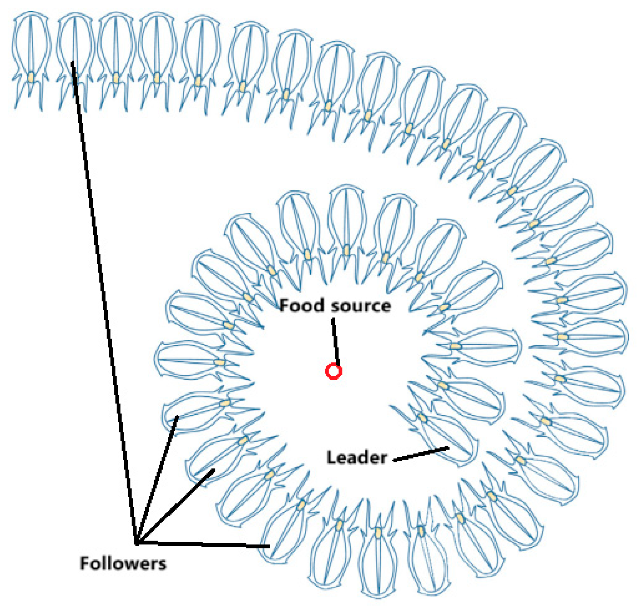
The SSA simulates the predation and movement behavior of salps, searching the solution space. During the iterative search process, the algorithm can explore broad regions, significantly improving the probability of finding the optimal solution. However, when SSA approaches potential optimal solution regions, its weak exploitation capability leads to excessive time required to thoroughly search these areas, resulting in slower convergence. Additionally, the multi-objective flexible job shop scheduling problem is a discrete optimization problem, whereas the original SSA is primarily designed for continuous scenarios and cannot be directly applied to discrete domains.

In order to apply SSA to the discrete domain, this paper first designs a double layer encoding mechanism. Then improve the SSA algorithm in terms of initialization strategy, global search strategy, and local search strategy to enhance its exploitation capabilities.

To address the application field limitation, this study first designs a conversion strategy between real-coded vectors and integer-coded vectors, expanding the algorithm’s applicability. It then integrates heuristic strategies such as the shortest processing time rule and the maximum remaining load rule to initialize the algorithm’s population. During iterations, tailored global and local search strategies are developed for process-sorting encoding and machine-selection encoding, aiming to enhance exploitation capabilities. The specific design of the improved algorithm is detailed below.

4.1. Double Layer Encoding Mechanism

FJSP-RPM requires addressing two subproblems: determining the processing sequence of workpieces on different machines and assigning each process to appropriate equipment. To solve this problem, a double-layer encoding mechanism is proposed. Each solution comprises two components: a workpiece-sorting encoding vector and a machine-selection encoding vector. Both vectors have lengths equal to the total number of workpieces to be processed in the workshop.

• Real-to-integer vector conversion:

The Ranked Order Value (ROV) is a data encoding method that converts continuous values into discrete sequences through ascending-order sorting and ordinal mapping. It is primarily used for scheduling optimization and continuous value discretization in algorithms. The standard procedure includes three steps: data sorting, ordinal assignment, and encoding conversion.

When decoding the real valued encoding vector to generate feasible scheduling schemes, the workpiece-sorting encoding vector is first transformed from the real-valued domain to the integer domain via ROV. For the machine-selection encoding vector, each value is multiplied by the number of available machines and then rounded to the nearest integer to determine the selected machine for the corresponding process.

As shown in

Table 2. An example of 3 jobs and 6 machines.

Workpiece	Production Process	Processing Information
		M1	M2	M3	M4	M5	M6
J1	O11	5		3		2
	O12		4		3		3
	O13					4	2
J2	O21		2		4
	O22	4		1			6
	O23		2		2	3
J3	O31	1		3	3
	O32	2	3
	O33			3		2	5

, a flexible workshop case involves three workpieces, each with a fixed process route. Multiple machines are available for each process, and processing times may vary across machines.

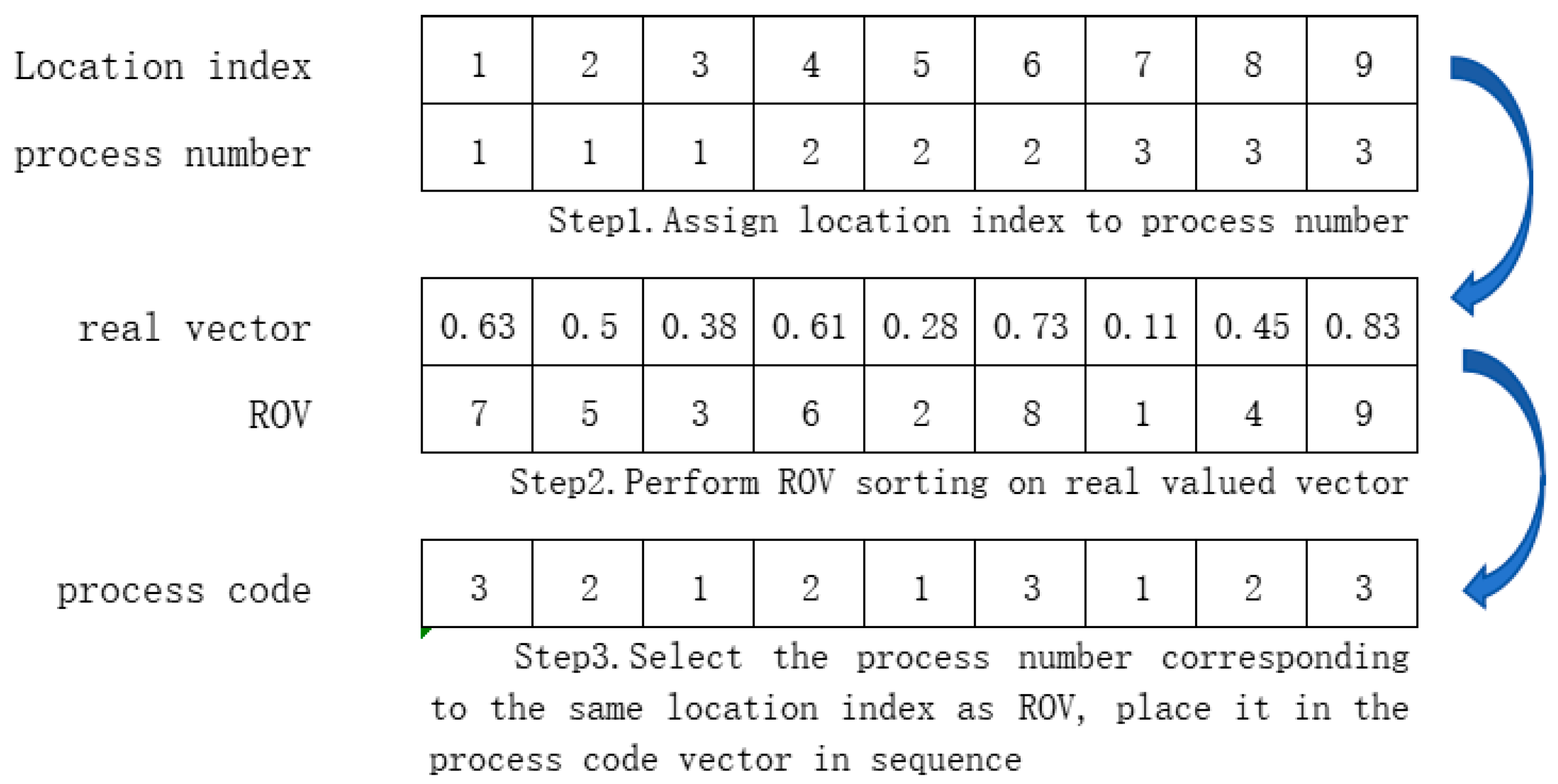
As shown in Figure 2, for the workpiece sorting encoding vector, we first assign a position index to workpiece process and then perform ROV sorting on the real-valued vector. Subsequently, process numbers sharing identical ROV values are selected sequentially from left to right and placed into the index positions corresponding to the integer-process encoding vector, thereby converting the real-number vector into an integer vector.

For example, when ROV is 7, the corresponding position of the workpiece process is the first process of workpiece 1. Similarly, the final integer form of the process code is [3 2 1 2 1 3 1 2 3]. Each number represents a workpiece, and the number of times it appears in the code represents the corresponding number of processes for that workpiece. For example, the first digit “3” in the encoding represents the first process of workpiece 3.

The machine selects encoding vectors and allocates them using the following formula:

$$m\left(i\right)=round\left({\displaystyle \frac{1}{2n}}\left(p\left(i\right)+n\right)\left(N\left(i\right)-1\right)+1\right)$$

(15)

Among them, $p\left(i\right)$ is the vector value at the ith position of the machine selection encoding vector, n is the total number of workpieces, $m\left(i\right)$ is the integer value at the ith position obtained by conversion, representing the machine number selected for the current process among the available processing machines, and $N\left(i\right)$ is the number of available processing machines for the current process.

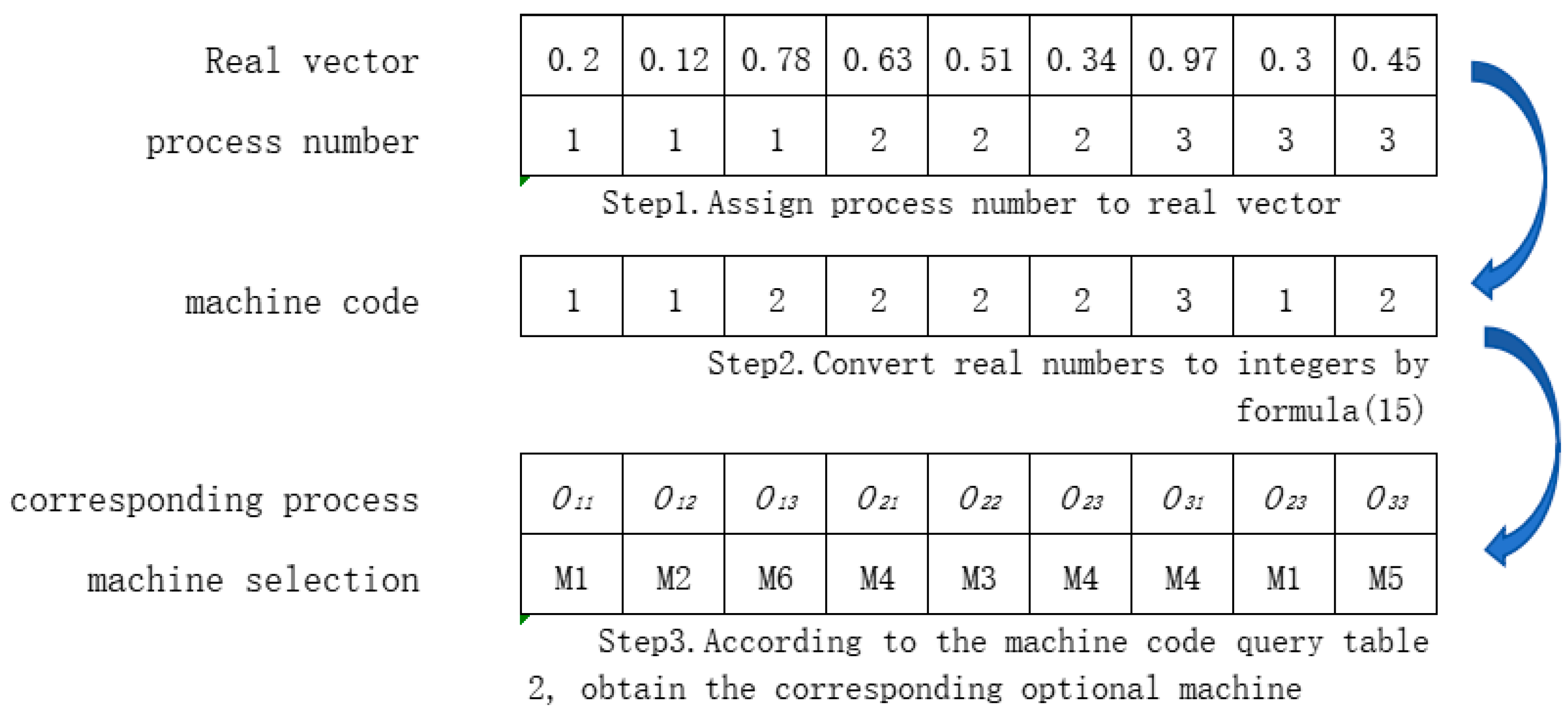
As shown in Figure 3, the machine selects the encoded real vector to correspond one-to-one with the process. Using Formula (15), the real vector is calculated and converted into an integer, representing the processing machine number selected for the corresponding process. For example, the first element 0.2 in the real number vector corresponds to the first process of workpiece 1. After calculation, the integer value “1” is generated, indicating that the first process of workpiece 1 is assigned to be processed by the first machine in the set of available processing machines. The available machines for the first process of workpiece 1 are $\left\{M_1, M_3,M_5\right\}$, so the machine $M_1$ is selected to perform this process.

• Integer-to-real vector conversion:

When converting the scheduling scheme into a position vector, for the machine selection encoding vector, the integer form of the machine selection encoding vector is converted into an individual position vector of the salp. The conversion formula is as follows:

$$x\left(i\right)=\left\{\begin{array}{c}{\displaystyle \frac{2M}{N\left(i\right)-1}}\left(m\left(i\right)-1\right)-M , N\left(i\right)\ne 1 \\ rand( ) , N\left(i\right)=1\end{array}\right.$$

(16)

Among them, $x\left(i\right)$ is the real value at the ith position of the machine selected encoding real vector, and $N\left(i\right)$ is the number of available processing machines for the current process. M is the total number of machines in the workshop, and $m\left(i\right)$ is the integer value at the ith position of the integer vector.

For the process sorting integer encoding vector, first generate a random number sequence with the same length as the vector, sort the random number sequence to obtain ROV1. For the process sorting integer encoding vector, assign the corresponding ROV value of the process code to ROV2 in order of the process number. And then find the random value in ROV1 that corresponds to the ROV2 value to obtain the real number encoding vector.

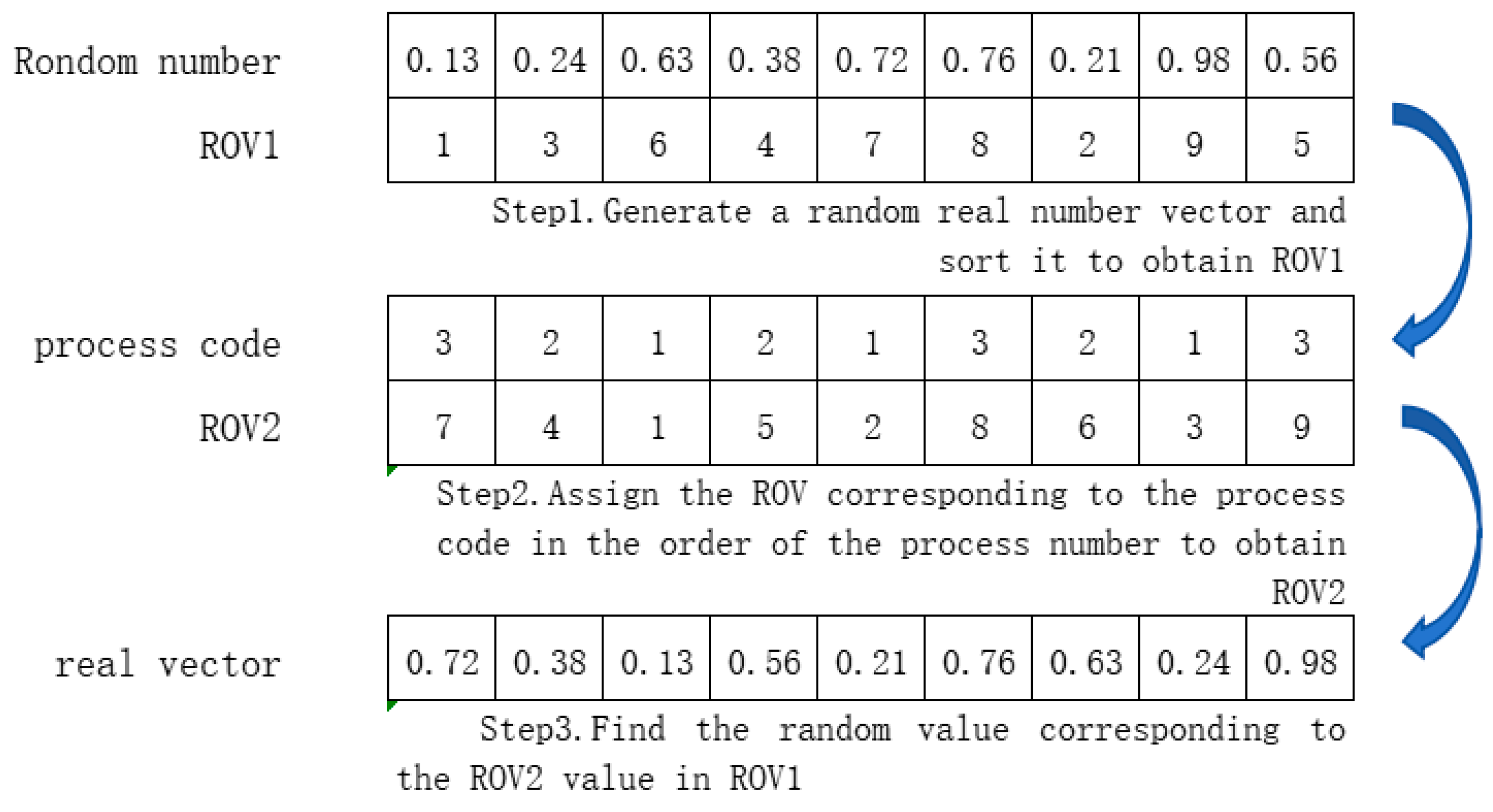
As shown in Figure 4, it is a schematic diagram of converting the process sorting encoding vector from an integer vector to a real vector. The initial process encoding integer vector is [3 2 1 2 1 3 2 1 3 3 3 3]. Based on the correspondence between the process encoding and position index shown in Figure 2, ROV2 is obtained. Afterwards, a set of random number vectors between 0–1 is generated [0.13 0.24 0.63 0.38 0.72 0.76 0.21 0.98 0.56], sorted to obtain ROV1. The first process of workpiece 3 corresponds to a value of 7 in ROV2 and a real number of 0.72 in ROV1. Therefore, the value at the corresponding position in the real number vector is set to 0.72. Following this method, the complete real number vector is calculated as [0.72 0.38 0.13 0.56 0.21 0.76 0.63 0.24 0.98].

4.2. Decoding and Individual Evaluation

After determining the processing sequence of orders across production lines, the active scheduling decoding method [26] is applied to decode the encoding scheme and derive the scheduling scheme. The quality relationships between solutions are evaluated using non-dominated sorting and crowding distance ranking methods.

4.3. Population Initialization

Population initialization constitutes a critical step in solving workshop scheduling problems, as the quality of generated solutions directly impacts the algorithm’s convergence efficiency and solution diversity. To ensure high-quality and diverse initial solutions, this study implements multiple initialization strategies for both machine selection and process sorting.

• Process code initialization strategy

  (1)

  Maximum residual load rule [27]: Workpieces are sorted in descending order based on the total residual processing time, prioritizing those with longer residual processing durations.

  (2)

  The shortest processing time rule [28]: Arrange the processes in ascending order of processing time, prioritizing the completion of processes with shorter processing times.

  (3)

  Random Selection Rule: Processes are randomly selected for machining without predefined criteria.

• Machine coding initialization strategy

  (1)

  The global selection rule [29] first creates an all zero array with a length equal to the number of machines, corresponding to the processing machines in the workshop. Then, a workpiece is randomly selected, and starting from the first process, the processing time of the available processing machines for that process is added to the array. The machine with the shortest processing time corresponding to the array position of the available processing machines for that process is selected as the current process processing machine, and the value of the corresponding position in the array is updated. The value of the array position corresponding to the machine not selected by the process remains unchanged. Repeat the above steps until the machine selection code is obtained.

  (2)

  The local selection rule [30] is basically the same as the global selection method, except that after determining the machining machines for all processes of a workpiece through the local selection method, the array will be reset to zero.

  (3)

  Randomly select rules. Randomly select machines from the set of optional processing machines for the process.

4.4. Global Search Strategy

The SSA does not rely on genetic operator evolution, but instead searches for the optimal individual of the problem through individual position movement. The advantage of this approach is that it can search for more space where potential optimal solutions may exist, but it will reduce search efficiency in workshop scheduling problems. Considering that genetic algorithms have strong global search capabilities, this paper combines crossover and mutation operators to improve the standard SSA and accelerate convergence speed.

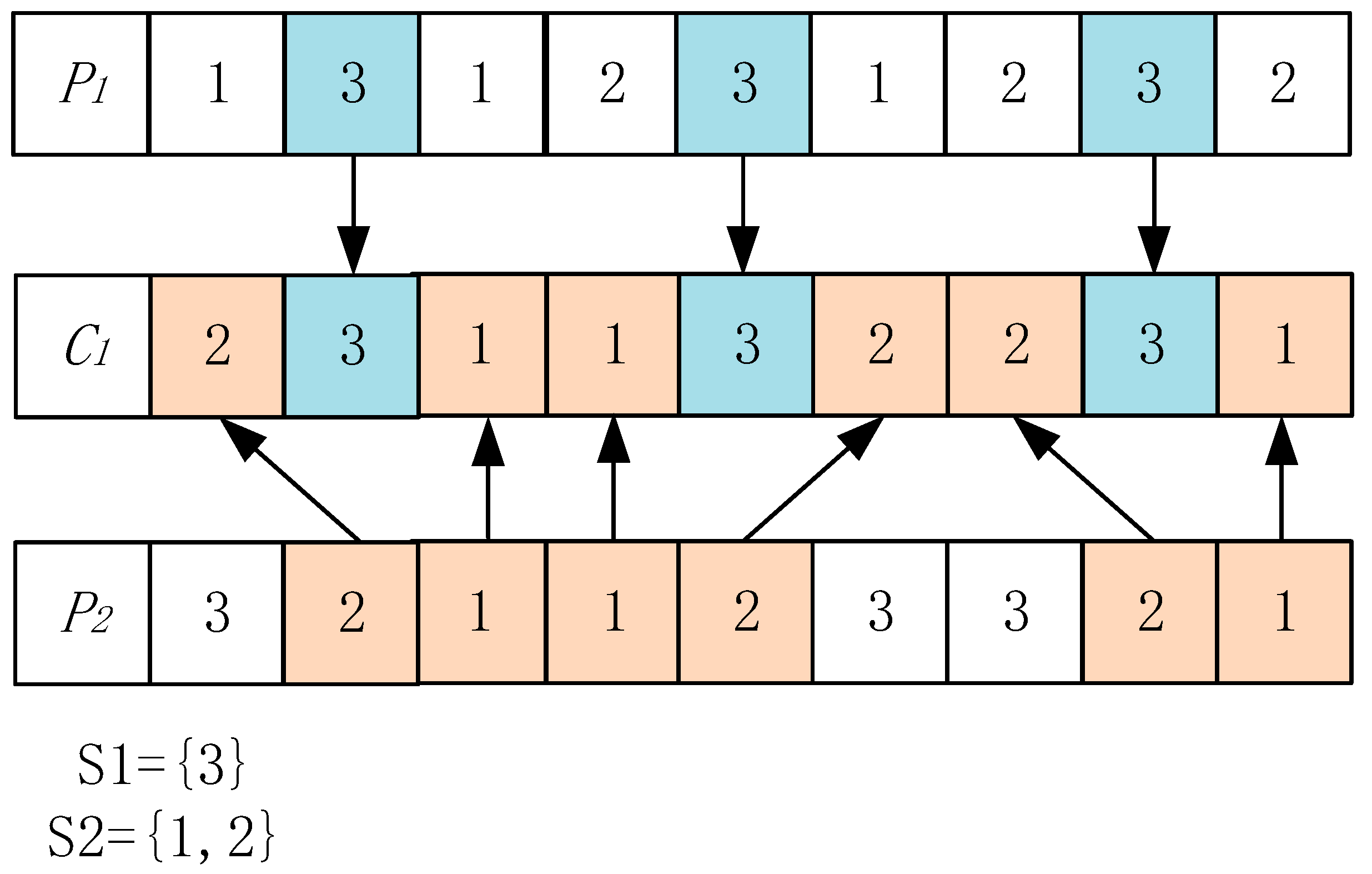
For the process sorting vector, choose the POX crossover method, as shown in Figure 5:

(1)

Divide the part set into two non empty subsets S1 and S2.

(2)

Copy the genes belonging to set S1 from the selected parent individual P1.

(3)

Fill the remaining positions in the offspring C1 with the genes from that belong to S2, preserving their order.

For the equipment selection part, a two-point crossover method is adopted:

(1)

Randomly select two crossover points for two parent individuals.

(2)

Exchange the equipment numbers corresponding to processes between the two crossover points in the parents to generate offspring.

4.5. Local Search Strategy

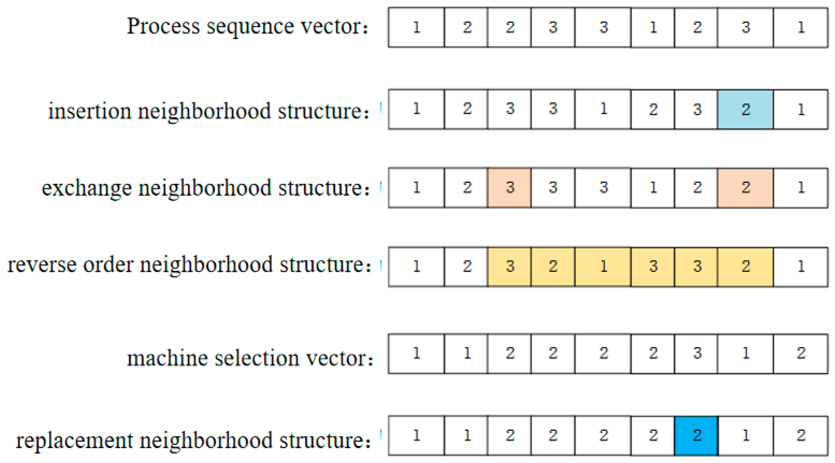
The SSA method employs a random search mechanism to explore the solution space by simulating the predation and mobility behaviors of salp populations, demonstrating strong global search capabilities. However, its drawback lies in prolonged search times when approaching regions containing potential optimal solutions due to the absence of effective local search strategies, resulting in poor convergence performance. To address this limitation, this paper proposes a variable neighborhood search strategy incorporating multiple neighborhood structures to enhance the algorithm’s optimization efficiency.

The specific neighborhood structure includes:

(1)

Swap Neighborhood: Randomly select two different positive integers, then swap the values at these two positions on the process sorting encoding vector to generate neighborhood solutions.

(2)

Insert Neighborhood: generate two different positive integers, insert the gene at the position of the first integer into the position of the second integer, and then adjust the order of process sorting encoding vectors.

(3)

Reverse Order Neighborhood: Within the interval between two generated unequal positive integers, reverse the order of all gene values within that interval.

(4)

Replace Neighborhood: Randomly select a parent machine to choose a process in the encoding, and replace the currently selected machine with other machines available for that process.

An example of neighborhood structure is shown in Figure 6. Since the problem considered in this article is a multi-objective optimization problem, in the process of variable neighborhood search, the decision to accept new neighborhood solutions will be based on the dominance relationship. The specific steps are as follows:

• Step 1: Define the neighborhood structure mentioned above.
• Step 2: Select a solution from the population in sequence for neighborhood search.
• Step 3: Use the above neighborhood structure to sequentially perform neighborhood search on the selected solutions and generate new neighborhood solutions.
• Step 4: Compare the dominance relationship between neighboring solutions and the current solution. If the neighboring solution dominates the current solution, then accept the neighboring solution and perform a new neighborhood search on the newly generated neighboring solution.
• Step 5: After all neighborhood searches are completed, stop the search for the current solution and repeat the process for the next solution in the population until all solutions have passed the neighborhood search.

By using a variable neighborhood search mechanism, the improved algorithm can thoroughly search for the neighborhood solutions of the current solution, greatly enhancing the algorithm’s local search capability.

The calculation process of the MISSA is shown in Algorithm 1:

Algorithm 1 MISSA Pseudo Code for Calculation Process

1 Begin

2 Initialize algorithm related parameters, including population size N, iteration times T, etc

3 Generate an initial population using an improved initialization strategy, calculate the fitness value of each individual, and rank non dominated relationships and crowding levels

4 Determine the optimal individual, namely the leader

5 Set the optimal individual as the food source

6 for t = 1:T

7   for i = 1:N

8     Convert integer encoding to real encoding,

9        if i == 1  %Update leader

10          Update the leader’s position using Equation (3)

11        else  %Update Followers

12        Update the following position using Equation (5)

13         end if

14     end for

15     Calculate the non dominated relationship and crowding degree between solutions, and update the population

16     Convert real number encoding to integer encoding

17     Using a global search strategy to update the population

18     Local search strategy updates population

19     Update optimal individuals and food sources

20 end for

21 Output the optimal frontier solution obtained from the solution

4.6. Comparison with Basic Salp Swarm Algorithm

This study introduces three enhancement strategies to the basic SSA: population initialization strategy, global search strategy, and local search strategy. The population initialization improvement strategy integrates residual load, shortest processing time, and global/local machine allocation rules to improve the quality of initial solutions; The basic algorithm is only randomly generated and of poor quality. The global search improvement strategy introduces POX crossover and two-point crossover to enhance search efficiency; The basic algorithm relies on random movement and converges slowly. The local search improvement strategy adopts variable neighborhood search (swapping/inserting/reversing/replacing) to improve local accuracy; The basic algorithm only randomly searches and is prone to getting stuck in local optima.

The improvement strategy enhances the quality of population initialization and strengthens the exploration capability of the algorithm. It can solve the shortcomings of slow convergence, susceptibility to local optima, and unstable solution quality of basic SSA in FJSP.

It is worth noting that, the mutual conversion between real vector and integer vector increases the computational cost of encoding/decoding. Integrating mechanisms such as POX crossover and variable neighborhood search also leads to an increase in runtime. However, for the test cases mentioned below, this increase in running time can be ignored considering the benefits it produces.

5. Simulation Experiment

In order to verify the performance of the algorithm, 10 test cases were designed. The data for each test case in the scheduling problem, such as processing time, delivery time, and rolling production cycle, are shown in

Table 3. Data of test cases.

Case	Quantity of Workpieces	Quantity of Machines	Delivery Date (min)	Scheduling Cycle
MK01	10	6	35, 30, 30, 30, 35, 35, 30, 30, 35, 35	34
MK02	10	6	20, 20, 20, 20, 20, 20, 15, 20, 15, 20	28
MK03	15	8	200, 180, 170, 180, 180, 175, 175, 180, 180, 175, 180, 180, 195, 190, 180	180
MK04	15	8	60, 50, 40, 30, 50, 70, 30, 40, 70, 30, 20, 40, 20, 15, 40	50
MK05	15	4	130, 120, 150, 140, 130, 160, 120, 150, 160, 160, 140, 130, 140, 140, 140	160
MK06	10	10	90, 75, 105, 80, 80, 85, 90, 75, 100, 105	100
MK07	20	5	90, 95, 100, 95, 105, 120, 110, 115, 105, 95, 115, 120, 115, 105, 90, 100, 105, 105, 100, 100	130
MK08	20	10	360, 400, 440, 370, 405, 365, 415, 395, 445, 390, 400, 385, 405, 400, 390, 395, 425, 385, 380, 380	400
MK09	20	10	290, 310, 290, 285, 340, 295, 345, 330, 290, 305, 280, 295, 295, 285, 310, 350, 320, 305, 330, 335	300
MK10	20	15	250, 270, 255, 245, 290, 240, 295, 285, 255, 265, 240, 250, 255, 235, 270, 305, 285, 245, 290, 295	300

. Program with MATLAB R2021b and run on an i7 processor with 3.3 GHz and 16 GB of memory. Select common NSGA2, NSGA3, and SPEA2 multi-objective optimization algorithms and compare them with MISSA. The algorithm performance indicators are calculated using convergence indicator GD (Generative Distance), diversity indicator Δ, and comprehensive indicator IGD (Inverted Generative Distance).

5.1. Parameter Design

The main experimental parameters that affect the performance of the MISSA include population size, number of iterations, and crossover probability. In order to determine the optimal parameter combination, this paper adopted the Taguchi orthogonal experimental method. A 3-factor 4-level experiment was designed:

• Population size: [40, 60, 80, 100]
• Number of iterations: [40, 60, 80, 100]
• Crossover probability: [0.6, 0.7, 0.8, 0.9]

For the IGD index (the smaller the better), key parameter effects were screened through 16 sets of experiments. Signal-to-noise ratio (SNR) is the core indicator used in Taguchi method to measure the performance of parameter combinations. Calculate the SNR for each set of parameters using the following formula. Each experiment was repeated 10 times (i.e., n = 10 in the formula) to eliminate random errors:

$$SNR=-10{\log }_{10}{\displaystyle \frac{1}{n}}\sum _{i=1}^n{IGD}_i^2$$

(17)

The results are shown in the

Table 4. Average SNR values at various parameter levels.

Parameter	Level	Average SNR (dB)	The Best
Population size	40	69.7
	60	71.3
	80	75.4
	100	80.2	√
Number of iterations	40	70.1
	60	73.3
	80	76.3
	100	79.6	√
Crossover probability	0.6	74.9
	0.7	76.4
	0.8	78.9	√
	0.9	78.8

:

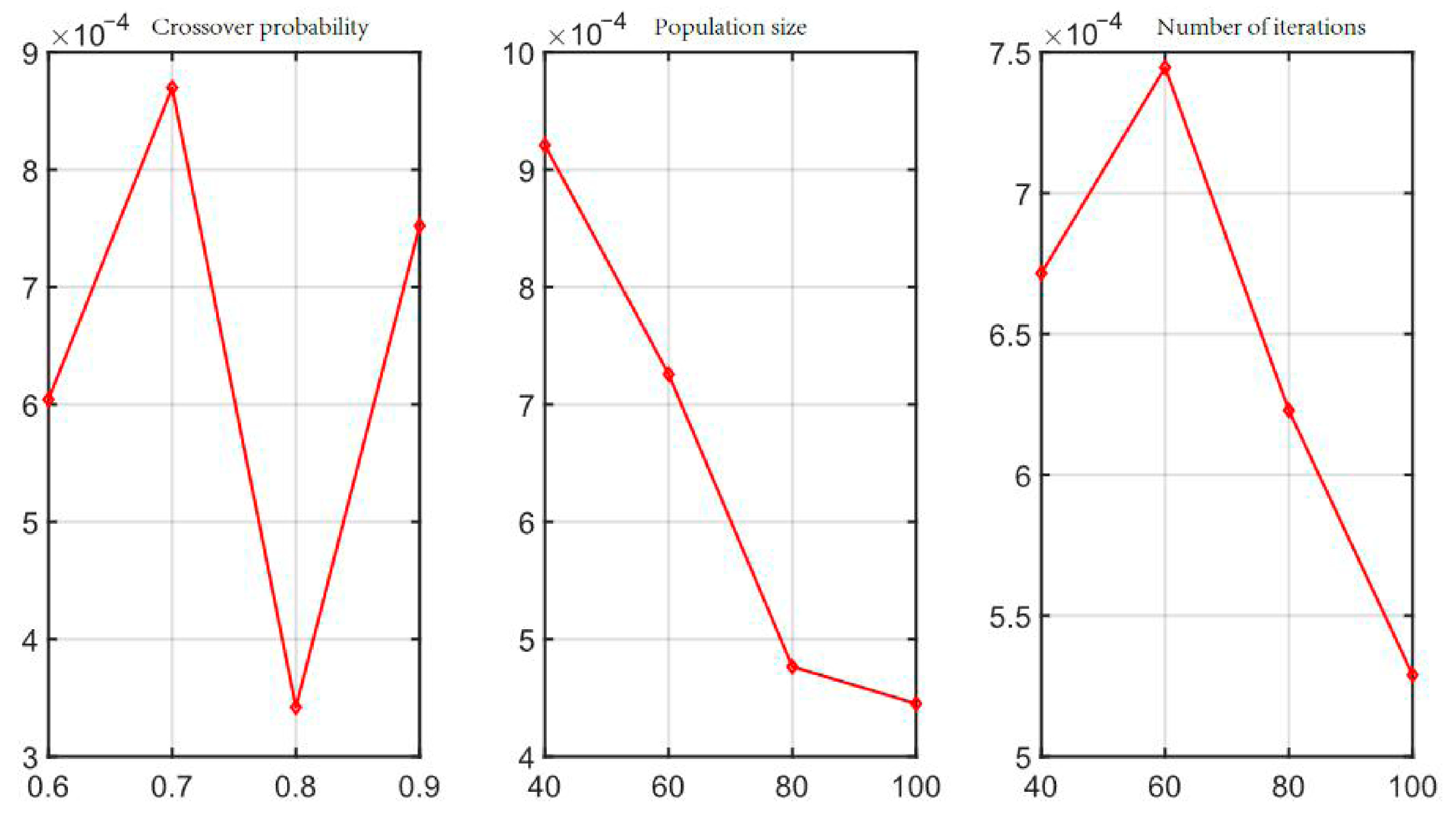
The parameter levels with the highest average SNR are: population size of 100 (80.2 dB); 100 iterations (79.6 dB); The crossover probability is 0.8 (78.9 dB).

To verify the above conclusion, the IGD index of the solution results was analyzed on the MK03 case. According to the experimental results shown in Figure 7, the optimal parameters for the MISSA algorithm were ultimately determined to be: population size: 100, number of iterations: 100, crossover probability: 0.8.

Table 5. Parameter variable setting.

Algorithm	MISSA	NSGA2	NSGA3	SPEA2
Population size	100	100	100	100
Number of iterations	100	100	100	100
Crossover probability	0.8	0.8	0.8	0.8

lists the initial parameter values for different algorithms for comparison of their performance.

5.2. Effectiveness Verification of Improvement Strategies

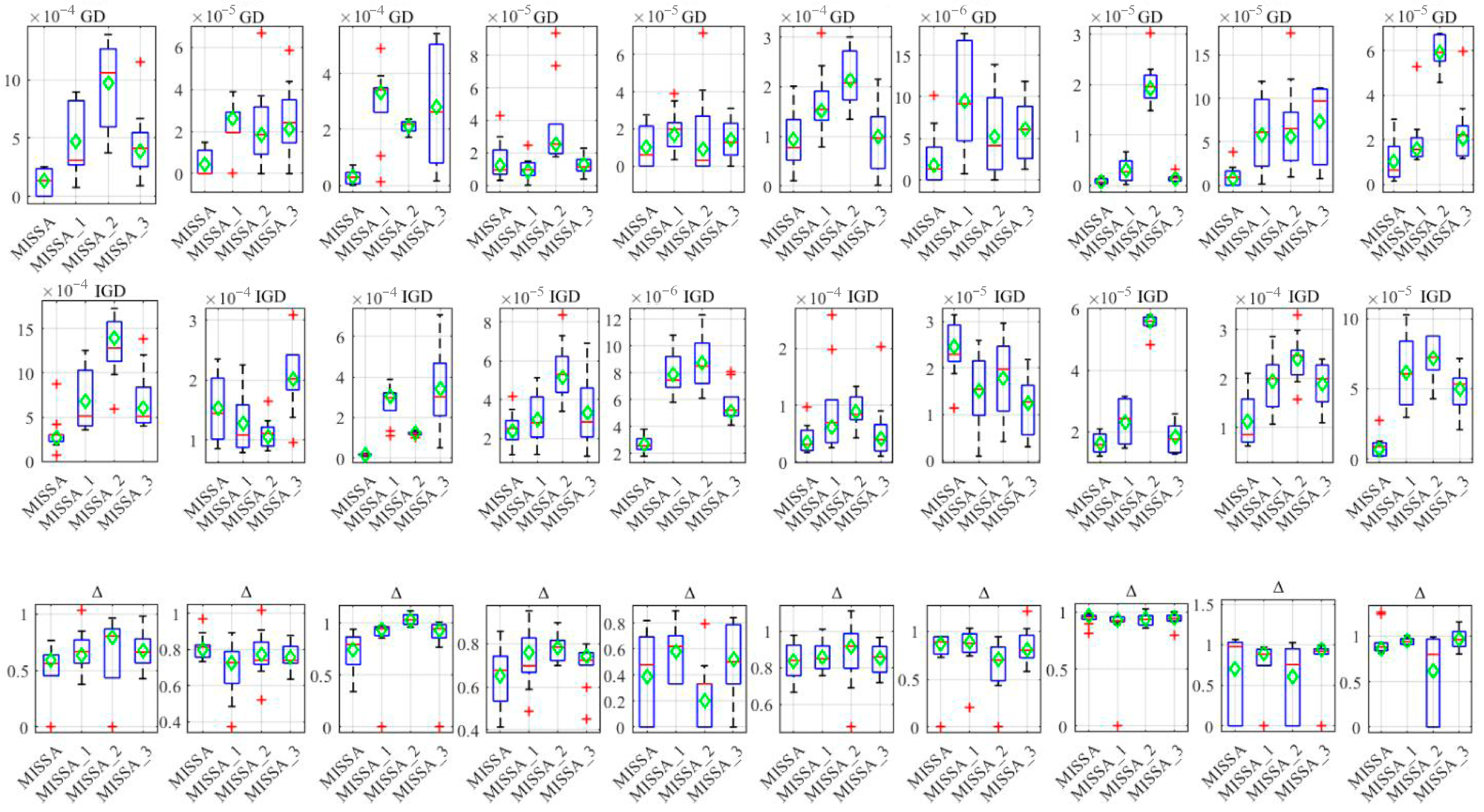
In order to verify the effectiveness of the proposed improvement strategy for the MISSA algorithm, three incomplete variants of the MISSA algorithm were designed, namely: ① MISSA_1, which introduces global and local search strategies on the basis of the original SSA, without including population initialization strategy. ② MISSA_2 introduces population initialization strategy and local search strategy, without including global crossover strategy ③ MISSA_3 includes population initialization strategy and global crossover strategy, but does not include local search strategy. For all cases, the algorithm is repeated ten times to eliminate the influence of policy randomness. To calculate the index values of the set solved by the algorithm, the solution sets obtained by the MISS A algorithm and its variants on the case are merged, and then sorted by non-dominated relationships to obtain the solution of the first dominated frontier. This first dominated frontier solution is then used as the optimal Pareto frontier solution set for the case. The performance of the algorithm was compared using three evaluation indicators, GD, IGD, and Δ. The comparison results are shown in

Table 6. Analysis of the Effectiveness of Algorithm Improvement Strategies.

Case	Index
	GD × 10−4				IGD × 10−4
	MISSA	MISSA_1	MISSA_2	MISSA_3	MISSA	MISSA_1	MISSA_2	MISSA_3	MISSA	MISSA_1	MISSA_2	MISSA_3
MK01	0.1309	0.4746	0.9723	0.4624	0.3218	0.6850	1.3172	0.6853	0.5307	0.6727	0.6333	0.6723
MK02	0.0044	0.0208	0.0233	0.0249	0.1526	0.1280	0.1109	0.2017	0.8181	0.6915	0.7706	0.7582
MK03	0.0310	0.2937	0.2126	0.2802	0.0167	0.2679	0.1207	0.3419	0.7460	0.8408	1.0342	0.8383
MK04	0.0151	0.0100	0.0370	0.0129	0.0256	0.0300	0.0548	0.0332	0.6501	0.7305	0.7831	0.6971
MK05	0.0104	0.0189	0.0155	0.0144	0.0027	0.0079	0.0088	0.0056	0.3863	0.5813	0.2593	0.5175
MK06	0.0936	0.1669	0.2138	0.1002	0.0398	0.0950	0.0890	0.0572	0.8383	0.8579	0.8733	0.8509
MK07	0.0026	0.0094	0.0052	0.0061	0.0233	0.0150	0.0178	0.0124	0.7823	0.8204	0.6320	0.8465
MK08	0.0008	0.0029	0.0203	0.0014	0.0160	0.0229	0.0552	0.0182	0.9401	0.8387	0.9367	0.9363
MK09	0.0104	0.0586	0.0675	0.0730	0.1129	0.1943	0.2407	0.1882	0.7049	0.7098	0.6060	0.7461
MK10	0.0102	0.0197	0.0592	0.0245	0.0090	0.0612	0.0716	0.0500	0.9377	0.9434	0.6129	0.9651

Among MISSA, MISSA_1, MISSA_2, and MISSA_3, the smallest value is bolded, indicating the optimal algorithm in this case.

and Figure 8.

Table 7. Comparison results of GD and IGD of MISSA, NSGA2, NSGA3 and SPEA2 algorithms.

Case	Index
	GD								IGD
	Mean Value × 10−4				Standard Deviation × 10−4				Mean Value × 10−4				Standard Deviation × 10−4
	MISSA	NSGA2	NSGA3	SPEA2	MISSA	NSGA2	NSGA3	SPEA2	MISSA	NSGA2	NSGA3	SPEA2	MISSA	NSGA2	NSGA3	SPEA2
MK01	0.2508	0.6781	0.9986	0.8567	0.1736	0.3446	0.3344	0.4410	0.2556	0.6555	0.9628	0.9053	0.1996	0.2389	0.4307	0.3992
MK02	0.0106	0.0169	0.0129	0.0157	0.0076	0.0156	0.0113	0.0170	0.0657	0.1122	0.0878	0.0858	0.0325	0.0470	0.0392	0.0279
MK03	0.0464	0.0483	0.0411	0.0290	0.0508	0.0276	0.0245	0.0164	0.0287	0.0607	0.0540	0.0480	0.0203	0.0296	0.0275	0.0212
MK04	0.0095	0.0204	0.0187	0.0145	0.0041	0.0120	0.0113	0.0127	0.0379	0.0751	0.0994	0.0644	0.0168	0.0280	0.0333	0.0228
MK05	0.0070	0.0182	0.0459	0.0160	0.0099	0.0188	0.0097	0.0156	0.0196	0.0134	0.0235	0.0125	0.0033	0.0104	0.0093	0.0155
MK06	0.0172	0.0372	0.0603	0.0220	0.0141	0.0336	0.0779	0.0194	0.0432	0.0548	0.0692	0.0492	0.0259	0.0253	0.0396	0.0279
MK07	0.0110	0.0067	0.0058	0.0037	0.0138	0.0070	0.0042	0.0032	0.0006	0.0011	0.0011	0.0007	0.0006	0.0013	0.0007	0.0005
MK08	0.0019	0.0025	0.0023	0.0028	0.0016	0.0012	0.0012	0.0026	0.0109	0.0107	0.0110	0.0139	0.0061	0.0030	0.0035	0.0057
MK09	0.0844	0.0967	0.1231	0.1218	0.0899	0.0212	0.0232	0.0207	0.0660	0.0927	0.1196	0.1220	0.0588	0.0175	0.0241	0.0189
MK10	0.0205	0.0328	0.0308	0.0229	0.0196	0.0134	0.0111	0.0134	0.0345	0.0391	0.0458	0.0375	0.0228	0.0127	0.0104	0.0136
Average value	0.0459	0.0958	0.1340	0.1105	0.0385	0.0500	0.0509	0.0562	0.0563	0.1115	0.1474	0.1339	0.0387	0.0414	0.0618	0.0553
Comparison	/	−52.0%	−65.7%	−58.4%	/	−22.2%	−24.3%	−31.5%	/	−49.5%	−61.8%	−58.0%	/	−6.5%	−37.5%	−30.1%
	The GD mean value is 52.0%, 65.7%, and 58.4% lower than other algorithms				The GD standard deviation is 22.2%, 24.3%, and 31.5% lower than other algorithms				The IGD mean value is 49.5%, 61.8%, and 58.0% lower than other algorithms				The IGD standard deviation is 6.5%, 37.5%, and 30.1% lower than other algorithms

Among MISSA, NSGA2, NSGA3, and SPEA2, the smallest value is bolded, indicating the optimal algorithm in this case.

lists the average values of ten solution results for MISS A and its variants on this test case, while Figure 8 shows the indicator value box plot of the ten solution results obtained by the algorithm. From Table 6 and Figure 8, it can be seen that compared with the algorithm variant, the GD index values obtained by the MISSA algorithm are superior to those of the algorithm variant in 9 cases, and have significant advantages in some cases such as MK01, MK02, MK03, and MK09. In terms of IGD indicators, MISSA also outperforms the comparison algorithm in 8 cases. In terms of diversity index Δ value, the performance of MISSA and MISSA2 algorithms is superior to the other two algorithms. The GD and IGD indicators obtained by the three algorithms MISSA_1, MISSA_2, and MISSA_3 have their own advantages in different cases, proving that each improvement strategy proposed in this paper can improve the overall performance of the improved algorithm. In terms of algorithm stability, the MISSA algorithm outperforms the three variant algorithms in terms of GD and IGD indicators of the solution results.

Based on the above analysis, each improvement item effectively improves the performance of MISSA in solving FJSP-RPM problems, and the effect is significant.

5.3. Comparison Between MISSA and Other Optimization Algorithms

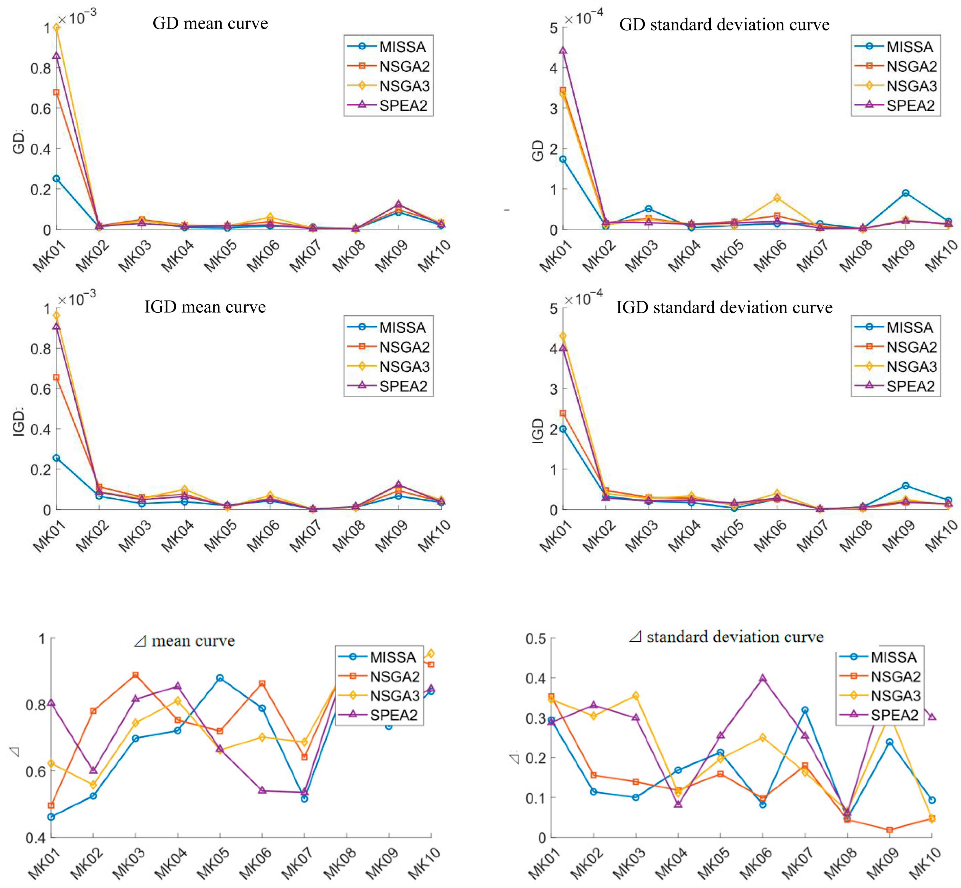
To verify the performance comparison between the MISSA and common multi-objective optimization algorithms such as NSGA2, NSGA3, and SPEA2, ten repeated comparison experiments were conducted on ten cases, and the performance indicators of the solution results were statistically analyzed. The comparison results are shown in Table 7 and

Table 8. Comparison results of of MISSA, NSGA2, NSGA3 and SPEA2 algorithms.

Case
	Mean Value				Standard Deviation
	MISSA	NSGA2	NSGA3	SPEA2	MISSA	NSGA2	NSGA3	SPEA2
MK01	0.4515	0.4955	0.6226	0.8036	0.3125	0.3533	0.3451	0.2879
MK02	0.5244	0.7803	0.5577	0.5994	0.1141	0.1557	0.3043	0.3309
MK03	0.6976	0.8888	0.7441	0.8155	0.1000	0.1392	0.3550	0.2992
MK04	0.7212	0.7530	0.8107	0.8540	0.1686	0.1178	0.1116	0.0807
MK05	0.8793	0.7195	0.6628	0.6649	0.2131	0.1590	0.1967	0.2543
MK06	0.7885	0.8633	0.7012	0.5399	0.0813	0.1978	0.2504	0.3981
MK07	0.5159	0.6412	0.6864	0.5353	0.2195	0.1800	0.1627	0.2540
MK08	0.8691	0.9290	0.9164	0.9280	0.0470	0.0440	0.0655	0.0605
MK09	0.7333	0.9652	0.8778	0.7886	0.2391	0.0185	0.3093	0.4163
MK10	0.8394	0.9198	0.9531	0.8463	0.0932	0.0474	0.0462	0.3000
Average value	0.7020	0.7956	0.7533	0.7376	0.15284	0.1620	0.2147	0.2682
Comparison	/	−11.8%	−6.8%	−4.8%		−5.7%	−28.8%	−43.0%
	The mean value is 11.8%, 6.8%, and 4.8% lower than other algorithm				The standard deviation is 5.7%, 28.8%, and 43.0% lower than other algorithms

Among MISSA, NSGA2, NSGA3, and SPEA2, the smallest value is bolded, indicating the optimal algorithm in this case.

and Figure 9 and Figure 10. Table 7 and Table 8 show the GD, IGD, and Δ index results obtained by the four algorithms. It can be seen from the table that compared with the other three algorithms, MISSA achieved smaller GD and IGD mean values in eight cases and smaller Δ mean values in seven cases in terms of solution quality, proving that the diversity and convergence of the solution set solved by MISSA are better. The quality of the obtained solution is higher. In terms of the stability of the solution results, it can be seen from the standard deviation data of different evaluation indicators in the table that the MISSA can achieve an absolute advantage, but still outperforms the comparison algorithm in a considerable number of cases.

To more clearly demonstrate the distribution of mean and standard deviation of indicators obtained through different algorithms for each test case, Figure 9 shows the distribution curves of mean and standard deviation of indicators obtained by four comparative algorithms. It can be clearly seen from the graph that the differences between different algorithms are small, but the performance of the MISSA in solving the set is superior to the comparison algorithm in the vast majority of cases.

To observe the distribution of the solution sets obtained by different algorithms more intuitively, Figure 10 shows the frontier solutions obtained by different algorithms, with points of different shapes representing the solution sets obtained by different algorithms. It can be clearly seen from the figure that the solution set solved by the MISSA basically dominates the frontier solutions obtained by the comparison algorithms, while the sets solved by the three comparison algorithms dominate each other, indicating that the solution set solved by the MISSA is closer to the Pareto frontier solutions of the case and has better solution set quality.

In summary, compared to NSGA2, NSGA3, and SPEA2 algorithms, MISSA has better global search and local optimization capabilities, and can more effectively solve the problems proposed in this paper.

6. Conclusions

This paper has made the following key progress through theoretical modeling and algorithm optimization:

1.

A flexible workshop scheduling model under rolling production mode was constructed with the goal of maximizing equipment utilization and minimizing total lead time. Effectively solved the coupling problem of equipment idle and order delay.

2.

Propose a conversion method between integer vector and real vector that is easy to operate, and apply the basic SSA to solve the discrete workshop scheduling problem.

3.

MISSA is proposed to solve FJSP-RPM more effectively than other algorithms. During population initialization, multiple heuristic strategies are designed to enhance the initial population quality, and the algorithm’s convergence speed is accelerated. By integrating the global crossover strategy with multiple local search strategies during the algorithm’s evolution, we enhanced the algorithm’s exploitation capabilities. Experimental results on the designed test cases demonstrate that MISSA reduced the mean values of GD, IGD, and by 52.0%/65.7%/58.4%, 49.5%/61.8%/58.0%, and 11.8%/6.8%/4.8% compared to NSGA2, NSGA3, and SPEA2, respectively.

This paper focuses on scheduling optimization in deterministic environments, assuming that production parameters (such as processing time, equipment status, etc.) are statically known quantities. In practical industrial scenarios, dynamic disturbances or random events may significantly affect the robustness of scheduling schemes. Although MISS A demonstrates strong global search capabilities in static problems, its adaptability in dynamic or real-time scheduling still needs further validation.