Article

An Improved Large Neighborhood Search Algorithm for the Comprehensive Container Drayage Problem with Diverse Transport Requests

College of Transportation Engineering, Dalian Maritime University, Dalian 116026, China
*
Author to whom correspondence should be addressed.
Appl. Sci. 2025, 15(11), 5937; https://doi.org/10.3390/app15115937
Submission received: 18 April 2025 / Revised: 20 May 2025 / Accepted: 23 May 2025 / Published: 25 May 2025

Abstract

:
Container drayage, as a pivotal element of door-to-door intermodal transportation, has garnered increasing attention due to its significant influence on container logistics costs. Although various types of transport requests have been defined in the literature, no comprehensive study has addressed all of them together yet, due to the lack of an efficient model and corresponding algorithms. Furthermore, existing research on container drayage often neglects the simultaneous incorporation of two trucking operation modes, two empty container repositioning strategies, and the availability of empty containers across multiple depots. To address these issues, this study proposes a comprehensive container drayage problem (CDP) and mathematically formulates it as an innovative mixed integer linear programming (MILP) model, capturing the uncertainty and unpredictability inherent in empty container allocation, truck dispatching, and route planning. Given the problem’s complexity, obtaining an exact solution for large instances is not feasible. Therefore, an improved large neighborhood search (LNS) algorithm is tailored by incorporating the “Sequential insertion” and the “Solution re-optimization” operations. Extensive numerical experiments using randomly generated instances of varying scales validate the correctness of the proposed model and demonstrate the performance of the proposed algorithm. Additionally, sensitivity analysis on the number and distribution of depots and empty containers offers valuable managerial insights for the development of an effective container drayage system.

1. Introduction

Container drayage refers to the short-distance transportation of containers using trucks, which has become an indispensable part of modern globalized supply chains and logistics networks. While container shipping covers long-distance transportation, drayage is responsible for connecting and transferring containers between container terminals and their customer locations, making it an essential link in the door-to-door service. Due to the limited capacity of trucks compared to container ships, the prosperity of container transportation has led to an increased number of trucks on the road, exacerbating traffic congestion and elevating carbon emissions [1]. Furthermore, despite its relatively short transport distances, drayage accounts for 25% to 40% of the total container transportation cost [2], while empty container transport makes up approximately 40% of drayage operations but generates no revenue [3]. As global trade volumes continue to rise, optimizing drayage operations has become increasingly critical to reducing overall transportation costs and carbon emissions, especially as demand for more efficient and sustainable solutions intensifies.
The optimization of container drayage operations essentially involves the allocation of empty containers, the dispatching of trucks, and the routing or sequencing of truck pickups and deliveries among container terminals, railway hubs, inland depots, and customers. Initially, the CDP was viewed as a one-to-one pickup and delivery problem in the pioneering research that began in 2002 [4], which is defined as picking up a container from a dedicated origin and delivering it to a specified destination. After this initial breakthrough, researchers soon recognized the significance of differentiating container status and flow direction, such as full or empty, inbound or outbound, resulting in eight types of common transport requests. Among these, six basic types of requests—inbound full (IF), empty repositioning (ER), empty demand (ED), outbound full (OF), inbound empty (IE), and outbound empty (OE)—refer to the transport of containers from an origin to a destination without intermediate nodes, while two types of composite requests—IFER and OFED—involve the combination of two basic requests. An IFER request requires an inbound full container to be delivered from a terminal (IF), and once emptied, the container must be repositioned to a depot or an alternative site (ER). On the contrary, an OFED request demands an empty container to be delivered to a shipper (ED) and after packing, the outbound full container should be delivered to the terminal (OF) [5]. IF, ER, ED, OF, IFER, and OFED requests are defined from the perspective of customer scheduling, while IE and OE requests are clarified from the standpoint of the shipping company. The handling of composite requests gives rise to two common trucking operation modes (Stay-with and Drop-and-pull) [6], while the combination of requests related to empty container repositioning and demand brings about two empty container repositioning strategies (Depot-turn and Street-turn) [7], both of which significantly increase the complexity of the CDP.
A large body of research has investigated the CDP in recent decades [8,9]. However, most existing studies focus on only a subset of these transport requests, which simplifies the modeling process but limits the model’s ability to reflect real-world practices. For example, Zhang et al. [10] considered four types of requests (IFER, OFED, IE, and OE) and developed a determined-activities-on-vertex (DAOV) graph-based model. Nevertheless, their model is too brief to explicitly describe the detailed drayage operations, especially the allocation of empty containers. Moghaddam et al. [5] constructed a generalized model for the CDP with four single requests (IF, ER, ED, and OF) and two composite requests (IFER and OFED), but they assume predetermined origins and destinations of all requests. Similarly, Yu et al. [11] also modeled the six types of requests where the destinations/origins of ER/ED requests are flexible, but their DAOV graph treats the terminal vertex as a bypass vertex and does not accommodate IE and OE requests. From the literature, the models considering IE and OE requests usually duplicate the terminal vertex according to the request number, while those not including IE and OE requests typically treat the terminal vertex as a bypass node or assume predetermined origins and destinations for all requests. To our knowledge, no study simultaneously incorporates the eight common types of requests into a single mathematical model, and thus, existing methods are not capable of solving them together. Additionally, most studies on the CDP focus on only one or two trucking operation modes and one or two empty container repositioning strategies. Furthermore, although half of the request types involve empty containers, researchers often ignore the scenario of multiple depots and the availability of empty containers [11]. To address this research gap, we are motivated to develop a DAOV-based model for the comprehensive CDP with diverse types of transport requests. The key contributions of this paper are threefold:
(1)
A comprehensive CDP is mathematically formulated as an innovative MILP model based on the DAOV graph, which is capable of simultaneously accommodating all types of transport requests, two trucking operation modes, two empty container repositioning strategies, and empty container constraints across multiple depots. Given the non-pairing of IE and OE requests, the forbidden arc is introduced into the model. Although there is only one terminal, it is handled in two distinct ways, depending on the request types. The terminal vertices of IE and OE requests are uniquely numbered to ensure that each request is executed, while those of IF/OF-related requests are ignored by using hyperarcs to reduce unnecessary arcs.
(2)
From a methodological perspective, the inherent complexity of the comprehensive CDP renders the attainment of an exact solution for industrial-sized instances highly challenging. To efficiently solve the problem, an improved LNS algorithm is developed by incorporating the “Sequential insertion” and the “Solution re-optimization” methods. The “Sequential insertion” method is responsible for converting the solution into multiple truck routes, while the “Solution re-optimization” method is used to refine the quality of solutions and ensure the feasibility of the truck routing plan.
(3)
The performance of the proposed LNS is evaluated by comparing it with MILP and GA for varying scale instances. The results not only demonstrate the effectiveness and efficiency of the LNS but also reinforce its potential as a more optimal approach in solving the problem at hand. Moreover, a sensitivity analysis is carried out to investigate the effect of the number and distribution of depots and empty containers, offering useful managerial insights for decision makers.
The remaining content of this paper is organized as follows. Section 2 provides a thorough review of the relevant literature. Following the problem description, Section 3 mathematically formulates the novel comprehensive CDP based on the DAOV graph. An improved LNS algorithm is designed in Section 4, and the MILP and the LNS are validated and evaluated through extensive randomly generated instances in Section 5. Finally, the paper is concluded in Section 6.

2. Literature Review

Over the past twenty years, extensive research has been conducted in the field of CDP, focusing on various types of requests as well as practical constraints and scenarios, including resource constraints, trucking operation modes, empty container repositioning strategies, multiple depots and multiple terminals, etc. [12]. This body of work has led to numerous significant insights through the exploration of the CDP and its various adaptations. In this section, we review the literature from the perspective of the types of transport requests addressed.
The CDP is essentially the pickup and delivery problem of containers. Wang and Regan [4] were the first to introduce the CDP supporting rail or maritime intermodal operations as the local full truckload pickup and delivery problem with time windows (FTPDPTW). In their study, there was only one type of container transport request, which was defined as picking up a container from a dedicated origin and delivering it to a specified destination. The FTPDPTW was modeled as a “multi-Traveling Salesman Problem with Time Windows” (m-TSPTW) using integer programming and solved by designing a heuristic algorithm that discretizes time window constraints. Following this initial breakthrough, the problem began to attract increasing attention from scholars and practitioners alike. Jula et al. [13] extended Wang and Regan [4] by proposing an exact algorithm based on dynamic programming for small size instances and a hybrid method combining genetic algorithms and dynamic programming for large size instances. To more accurately capture the practical scenarios or constraints encountered by the Korean trucking industry, Chung et al. [14] developed several variants of the basic model presented in Wang and Regan [4] by considering multi-size containers, heterogeneous fleets, and vehicles with different ownership, and solved them with an insertion heuristic. Furthermore, Vidović et al. [15] formulated a generalized multiple matching problem model applicable to any type of vehicle capable of simultaneously transporting multiple 20 ft and 40 ft containers, while Yang and Daham [16] modeled the pickup and delivery process of 20 ft and 40 ft containers with heterogeneous fleets as a MILP. To solve larger instances, the former designed a variable neighborhood search (VNS) heuristic, and the latter proposed a decomposition and aggregation heuristic. Recently, Bruglieri et al. [17] established a more practical variant of the CDP with release and due dates by considering the multi-trip multi-period features and designed combinatorial Benders’ Cuts methods. Since the haulage of more than one multi-size trailer by a truck is legal, Bjelić et al. [18] focused on solving a dynamic multi-size multi-trailer CDP with a rolling-horizon approach. Aiming at handling the requests with uncertain arrival times, Jia et al. [19] designed a Markov decision process model for the CDP and combined reinforcement learning with integer programming to solve it. With the emergence of e-commerce drayage platforms, traditional drayage operations are facing new challenges. Thus, Chen et al. [20] investigated a dynamic drayage container booking and routing problem with regular and flexible requests. Against the backdrop of the “dual carbon” goal [21], electric trucks hold the promise of tackling climate-related issues. Hence, Xiao et al. [22] introduced electric trucks into the CDP, considering charging resource constraints. They developed an improved adaptive LNS algorithm by combining it with an exact method.
However, the above articles did not clearly distinguish between inbound and outbound containers, nor did they differentiate between empty and full containers. In practice, after an inbound full container is unpacked at its consignee location, an empty container will be left behind which can be moved back to a terminal, a depot or a shipper demanding an empty container. In contrast, before an outbound full container is packed at the shipper location, an empty container should be delivered to it from a terminal, a depot or a consignee. To efficiently use the emptied containers resulting from inbound full containers, empty container repositioning in the CDP has garnered greater attention.
In some studies, the terminal is regarded as the storage place of empty containers instead of the inland depot, while the depot is just a truck or trailer parking site. Aiming at this scenario, Imai et al. [7] introduced a Street-turn strategy by defining two types of transport requests: delivery request and pickup request. The former refers to delivering an inbound full container to a consignee from a terminal and transporting back the emptied container after unloading cargoes, while the latter requires delivering an empty container to a shipper from a terminal and hauling back the outbound full container after loading. The two requests are actually the variants of IFER and OFED requests. They paired each delivery request with a corresponding pickup request, thus transforming the problem into a single-stop backhaul problem, where one truck could handle both the delivery and pickup operations in a single trip, and proposed a sub-gradient heuristic based on Lagrangian relaxation. Caris and Janssens [23] refined the problem of Imai et al. [7] to a FTPDPTW by adding time window constraints for the requests. Lai et al. [24] considered a multi-size container version of Imai et al. [7], and proposed a two-stage metaheuristic. Ghezelsoflu et al. [25] designed a set-covering model by relaxing the restriction that all consignees were served before all shippers in Lai et al. [24]. Since pickups at customer locations did not need to be considered in these studies, the Stay-with mode was only applicable. To make the scheduling more flexible and increase the utilization of trucks/tractors, the Drop-and-pull mode that allowed the separation of trailers or containers from tractors or trucks was employed in the following three articles. Xue et al. [26] allowed the separation of tractors from trailers, and constructed a tabu search algorithm. While trailers may be left at customer locations, it is essential to ensure that the trailer depot has enough trailers to maintain normal operations. As a result, trailer repositioning was incorporated into the CDP with multi-size containers and heterogeneous fleet by Cui et al. [2], and a hybrid heuristic combining LNS and tabu search (TS) was developed to solve the proposed two-stage model. Wang et al. [27] addressed a drayage problem that a tractor can pull multiple trailers with an adaptive LNS algorithm. Focusing on the interference of tractors, Wang et al. [28] proposed a CDP with controllable vehicle interference and designed a branch-price-and-cut algorithm to solve the MILP model. With the advancement of automatic vehicle and wireless communication technologies, You et al. [29] introduced a general semi-autonomous truck platooning mode for the CDP where one customer can be served by two different truck platoons. Xue et al. [30] extended the work of You et al. [29] by considering the effect of fuel saving and proposed a TS heuristic. To overcome the issue that each driver must be attached to their leading truck in previous studies, Yan et al. [31] introduced an improved platooning operation mode for the CDP, where the drivers can move by alternative transport modes, such as taxis, to perform subsequent tasks, while You et al. [32] proposed a similar multi-trip CDP with platooning operation mode. The former designed a simulated annealing-based heuristic and the latter developed a Branch-and-Price-and-Cut algorithm. To expedite the processing of trucks, some terminals start to employ truck appointment system. Huang et al. [33] integrated truck appointment system into the CDP, and introduced a tailored GA to solve the problem. Due to the ignorance of workload balance in previous studies, Wang et al. [34] proposed CDP that simultaneously incorporates the Drop-and-pull mode and the route balancing. It is worth to note that both Huang et al. [33] and Wang et al. [34] split the IFER and OFED requests into four basic requests, i.e., IF, ER, ED, and OF.
Aside from container terminals, in reality, the empty containers generated by unpacking inbound full containers may have multiple destinations, including depots or shippers. Additionally, not every delivery request can be perfectly paired with a pickup request. Consequently, the repositioning of empty containers was formally introduced into the study of CDP by Zhang et al. [35]. They pioneered the extension of previous studies by incorporating four types of transport requests: IFER, OFED, IE, and OE, laying the foundation for subsequent research. Since the destination of the IE request and the origin of the OE request are not given in advance, the IE/OE requests are also called flexible requests. Additionally, they exclusively employed the Stay-with mode, formulated a multi-depot CDP as a MILP model based on a DAOV graph and developed a reactive TS algorithm. Nevertheless, they treated the determined movement between a request vertex and any other vertex as the activity on the request vertex, making the time calculation more complex and difficult to explicitly describe the allocation of empty containers. Zhang et al. [36] and Nossack and Pesch [37] further extended Zhang et al. [35] to a CDP with multiple depots and multiple terminals. The latter designed a two-stage heuristic that outperformed the window partitioning method proposed by the former. Sterzik and Kopfer [38] explicitly modeled the repositioning of empty containers upon the framework presented by Zhang et al. [36], and designed an enhanced TS heuristic, demonstrating superior effectiveness and efficiency on both small and large instances compared to existing methods. Braekers et al. [39] investigated the scenario of one vehicle depot and multiple terminals where terminals are used to store empty containers, and proposed a sequential and an integrated approach, but their model only allowed the Drop-and-pull mode for IFER requests. Zhang et al. [40] investigated the CDP with multi-size containers utilizing a state-transition-based modeling method and improved reactive TS algorithm. However, they made the “full-twin” assumption, which states that if a truck is carrying two 20 ft full containers, it can only begin transporting new requests after unloading both of them. Zhang et al. [10] formulated a bi-objective mathematical model based on the DAOV graph by considering empty containers constraints and designed a LNS algorithm to solve the problem. Funke and Kopfer [41] relaxed the “full-twin” assumption in Zhang et al. [40] by introducing a MILP model. Yang et al. [42] extended Funke and Kopfer [41] by considering heterogeneous fleet and network flow constraints at depots, and solved this problem using a tailored generic algorithm (GA). However, the trucks were forced to start/finish at the terminal which reduced the difficulty of modeling.
Due to trade imbalances, certain regions have become import-dominant or export-dominant areas where inbound empty and outbound empty containers may not exist simultaneously. Zhang et al. [43] then focused on the CDP in an export-dominant area, and restricted the three types of requests: IFER, OFED, and IE. Since the purchase cost of empty containers is relatively high, which means the supply of empty containers in container terminals or inland depots is not inexhaustible. Therefore, for the CDP, empty containers are also a necessary transportation resource, in addition to the two essential resources of trucks and drivers found in typical vehicle routing problems. Zhang et al. [43] first formulated the CDP with empty container constraints as a m-TSPTW and developed a reactive TS algorithm to solve it. Conversely, Song et al. [6] examined the CDP under a Drop-and-pull mode with three types of requests: IFER, OFED, and OE, restricting the same truck to picking up the separated container. The IFER request was further divided into two types according to the status of the emptied containers. If the emptied container released by the IFER request needs maintenance, it must be moved back to the depot; otherwise, it can be moved to any location where an empty container is needed or can be stored. They proposed a branch-and-price-and-cut algorithm to optimally solve the problem. Subsequently, Song et al. [44] added empty container constraints to their previous study. Huang and Zhang [45] simultaneously modeled the CDP involving requests of IFER using foldable/standard containers, OFED, and IE under foldable state at the terminal and designed a LNS algorithm. The container type in an OFED request needs to be decided apart from the general decision variables in the CDP.
When considering the inbound full or outbound full containers, the aforementioned studies always take into account the repositioning or pre-delivery of empty containers. However, due to limited equipment or time, sometimes an inbound full container may not be unpacked on the same day it is delivered, while an empty container delivered to the consignee may not be packed on the same day. Therefore, the basic requests, such as IF, ER, OF, and ED, should also be taken into consideration. Moghaddam et al. [5] constructed a generalized model for the CDP by considering six types of requests: IF, ER, ED, OF, IFER and OFED, but they assumed predetermined origins and destinations of all requests which reduced the complexity and applicability of the model. Similarly, Yu et al. [11] also modeled these six types of requests, with the destinations/origins of ER/ED requests being flexible, but their DAOV graph treats the terminal node as a bypass node and thus does not accommodate IE and OE requests. Additionally, Fazi et al. [12] investigated six types of requests, encompassing five of the common requests (IF, ED, OF, OFED, and IFER), along with a special request type—IFOF. An IFOF request means a customer receives an inbound full container and immediately releases an outbound one, which can be easily split into an IF and an OF request because of no dependency on the operational sequence. Given that the terminal vertex must be visited for full container-related requests, they treated it as a bypass node in order to minimize the number of arcs.
From the literature, it can be seen that many studies have investigated CDP with various types of requests, considering practical constraints (time window, capacity, and the availability of empty containers), trucking operation modes (Stay-with and Drop-and-pull), empty container repositioning strategies (Depot-turn and Street-turn), operational scenarios (multiple depots and multiple terminals), and the employment of new technologies (semi-autonomous truck platoon, electric truck, and e-commerce platform). While the pioneering work of the CDP and its variants focused on the pickup and delivery problem [13,14,15,16,17,18,19,20,21,22], they did not differentiate between the detailed types of requests. To improve clarity, Table 1 summarizes the problem characteristics identified in closely related studies on the CDP, with a focus on differentiating request types.
A comparison of the existing literature reveals that these studies bear the most resemblance to our research. However, the models for the CDP considering IE and OE requests usually duplicate the terminal vertex according to the request number, while those not including IE and OE requests typically treat the terminal vertex as a bypass node. To the best of our knowledge, there is no study that simultaneously incorporates the eight common types of requests into a single mathematical model. Additionally, most existing studies on the CDP focus on only one or two trucking operation modes and one or two empty container repositioning strategies, often ignoring the scenario of multiple depots and the availability of empty containers. These limitations restrict the model’s ability to accurately reflect real-world practices. Therefore, this study proposes a comprehensive CDP which is capable of simultaneously accommodating all types of transport requests, two trucking operation modes, two empty container repositioning strategies, and empty container constraints across multiple depots, and designs an improved LNS to efficiently solve it.

3. Problem Definition and Formulations

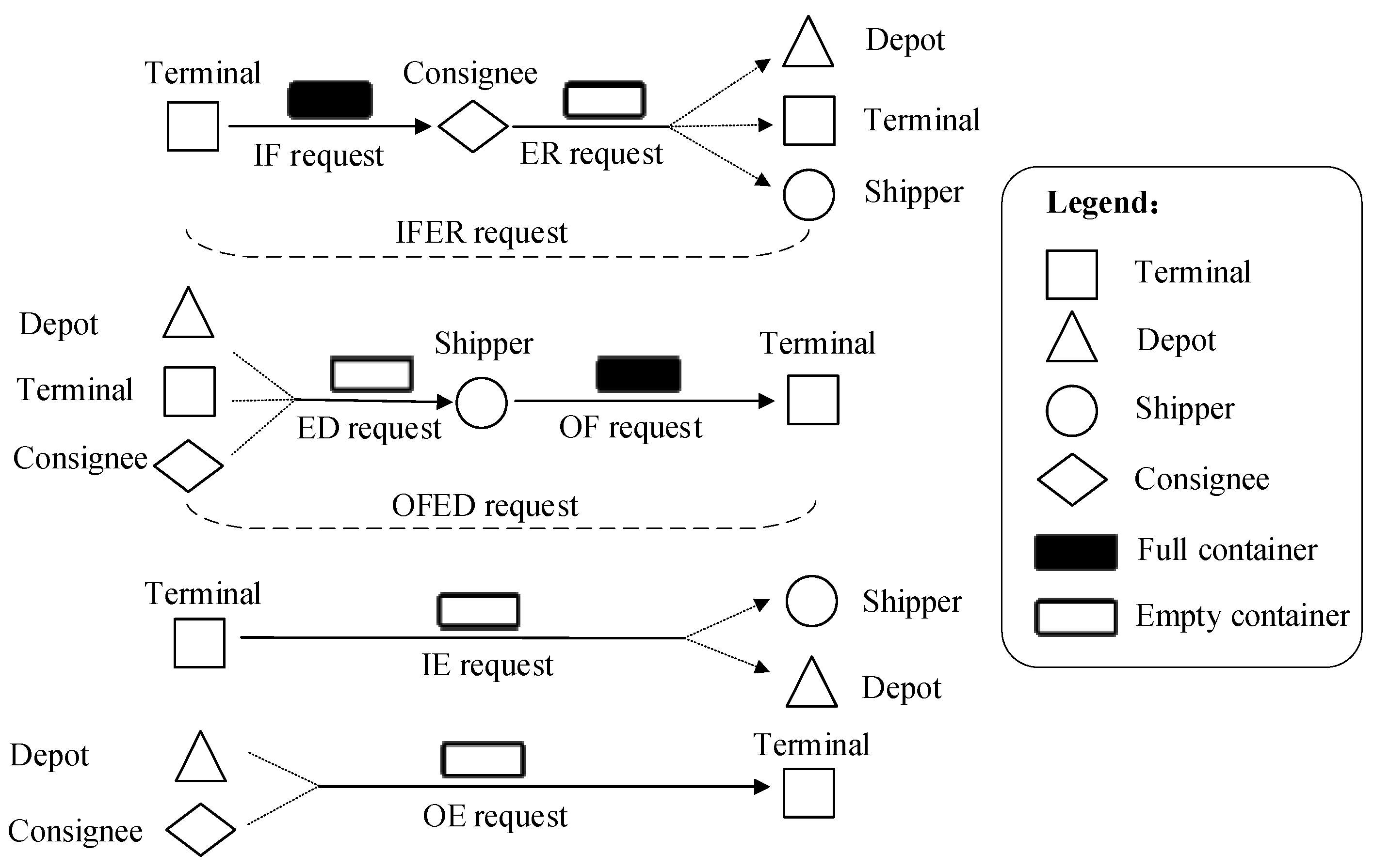
3.1. Problem Description

The comprehensive CDP with diverse types of transport tasks is defined as follows. A container transport company possesses a limited fleet of homogeneous trucks to serve container transport requests issued by customers (shippers and consignees) and shipping companies between the container terminal, multiple depots, and customers. The company manages multiple depots that can provide empty containers and serve as parking places for trucks. Because of the elevated expense associated with acquiring empty containers, the stock level of empty containers at each depot is finite and fluctuates dynamically as trucks pick up empty containers from the depot or deliver them back to it. The truck must depart from a depot and return to any depot by the end of the day. Each truck can only carry one container at a time, with all containers being of identical size. Each request is constrained by distinct time windows. The objective of the problem is to simultaneously optimize empty container repositioning, truck scheduling, and route planning to deal with all requests.
A request in this study is defined as a container transport task issued by customers (shippers and consignees) or shipping companies. The eight types of requests consist of six basic requests (IF, ER, ED, OF, IE, and OE) and two composite requests (IFER and OFED), as illustrated schematically in Figure 1:
(1)
IF request: This requires hauling the inbound full container from the terminal (Origin) to the consignee (Destination). This kind of request is very common, as sometimes a container cannot be unpacked on the same day as it is delivered, and the emptied container will need to be picked up the other day.
(2)
ER request: This refers to hauling back the emptied container from the consignee (Origin) to the terminal, a depot, or a shipper demanding an empty container after an IF container has been unpacked. The destination of an ER request is flexible, thus offering potential for optimization at the operational level.
(3)
ED request: This involves hauling an empty container from a terminal, a depot, or a consignee to a shipper (Destination) demanding it. The ED request is not always combined with OF request, as the empty container may not be packed immediately after its arrival, and thus the loaded container transport request can only be submitted afterward.
(4)
OF request: This specifies hauling the outbound full container from the shipper (Origin) to the terminal (Destination).
(5)
IE request: This entails hauling the inbound empty container from the terminal (Origin) to a depot or a shipper who demands it. However, the destination of an IE request cannot be the terminal. If the destination is the terminal in a one-terminal scenario, the transportation will be handled by internal or in-port trucks, which are not managed by the trucking company.
(6)
OE request: This implies hauling the outbound empty container from a depot or a consignee to the terminal (Destination). The IE and OE requests are submitted by shipping companies due to the requirement of empty container repositioning between different terminals or regions.
(7)
IFER request: This is a composite request, which means that a consignee requires an IF container to be picked up from the terminal and delivered to their location, and the empty container to be picked up immediately after unpacking and repositioned to a suitable place.
(8)
OFED request: This is also a composite request, which indicates that a shipper requires an empty container to be delivered from the location where it is available to their location, and the OF container to be picked up immediately after packing and finally delivered to the terminal.
Although an ER and an OE request may share the same origin and destination if they can be paired with each other, they should still be treated as individual requests. The service time windows at the customer locations for requests such as IF, ER, ED, OF, IFER, or OFED, and at the terminal for requests like IE or OE are known in advance. If a request issued by a single customer or a shipping company involves more than one container, it will be divided into separate requests, each corresponding to a single basic transport request with the same service time window. For composite requests, two trucking operation modes, i.e., Stay-with mode and Drop-and-pull mode, are allowed to facilitate more flexible and efficient truck scheduling. Regarding requests relating to empty container repositioning, both the Depot-turn and Street-turn strategies are viable, provided they minimize unnecessary detours effectively.
The availability of empty containers across multiple depots, coupled with diverse types of requests, two trucking operation modes and two empty container repositioning strategies, significantly increases the following uncertainty and unpredictability of empty container allocation, truck dispatching, and route planning. First, when selecting a depot for truck dispatch to serve empty container-related requests, two key factors must be considered: the distance between the depots and the request vertex, and the dynamic number of available empty containers and trucks at each depot. A straightforward approach of selecting the nearest depot is not feasible in this context. Furthermore, when handling a composite request, the combination of Stay-with and Drop-and-pull modes may result in three potential dispatch configurations: (i) a single truck uninterruptedly completes its delivery and pickup parts; (ii) a single truck completes its delivery and pickup parts, but in between, the truck departs to handle other requests; and (iii) two trucks are assigned to separately handle the delivery part and pickup part. Thus, the sequence of trucks cannot be predetermined for composite requests. In addition, with respect to the ER/ED request, only one of the origin and destination is known, while the other needs to be determined based on the Street-turn and Depot-turn strategies during optimization. Similarly, for the IE/OE request, only one of the origin and destination is known and the other should be identified based on the optimization model. In summary, the inherent uncertainty and unpredictability associated with the decision of empty container allocation, truck dispatching and route planning must be explicitly incorporated into the model, thereby posing substantial challenges to the model process and its solution.

3.2. Graphical Formulation

3.2.1. The DAOV Graph

Although the comprehensive CDP shares some similarities with the VRP in vehicle scheduling and route planning, it also has distinct characteristics, notably the requirement that flexible requests involving empty container transportation should be simultaneously considered with the planning of truck routing. The uncertainty and unpredictability mentioned in Section 3.1 obviously increase the complexity of this problem, which makes it difficult to directly establish a mathematical model. To address this issue, this study graphically formulates the proposed problem based on a DAOV graph.
A DAOV graph G = N , A comprises a set of vertices N and arcs A. Note that N = N r N d , where N r is the set of request vertices, and N d is the set of depot vertices. A vertex refers to not only the physical node, but also the determinate activities that occur at that node. For example, a depot vertex stands for both the depot node and the activity of departing from or returning to the depot; as such, it is termed the departure or return vertex. Similarly, for a basic request, its vertex denotes either the customer location (for IF, ER, ED, and OF requests) or the terminal (for IE or OE requests), and encompasses the associated pickup or delivery activities at these sites. However, for a composite request, since it involves both the delivery and pickup activities at the customer location, representing it with a single request vertex will render the Drop-and-pull mode inapplicable. To accurately model this type of request and effectively implement the Drop-and-pull mode, it is imperative to split the composite request into two sequential vertices: a delivery request vertex and a pickup request vertex. The delivery request vertex must be served prior to the pickup request vertex, with the service start time of the pickup request not occurring earlier than the service completion time of the delivery request.
Based on the classification of request types and the split of composite requests, four types of request vertices can be formulated, and thus, N r = N D E C N D F C N P E C N P F C . The activities that may be performed at each type of request vertex are shown in Table 2. An arc i , j in set A is responsible for connecting two different vertices in set N, which corresponds to the truck scheduling-related indeterminate activities that should be determined by the optimization process. The activities and transfer time on arcs are illustrated in Table 3. The number 0 in Table 3 denotes the terminal when it serves as a bypass vertex/node, while t 0 is the time required for loading or unloading a container at the terminal, and t i 0 ( t 0 j ) is the travel time from vertex i (0) to 0 (j).

3.2.2. Network Flow Constraints

As shown in Table 3, there is no direct arc between depots because empty containers are usually transported between the terminal, depots, and customers. The balance of empty containers at various depots can be handled during the scheduling process, and thus the unprofitable transportation of empty containers between depots is prohibited. Additionally, there is also no direct arc between identical vertices. In such cases, the truck is essentially waiting at that vertex, which can be explicitly reflected in the model.
In addition to the common arcs that are disallowed in Table 3, there is also a special arc for the IE and OE requests, referred to as the forbidden arc. The forbidden arc indicates that no flow is permitted from an IE request vertex to an OE request vertex. If an IE request is paired with an OE request, then the transportation of the empty container within the terminal is, in essence, a transshipment operation that can be carried out by an internal truck. This, however, falls outside the scope of our study. Therefore, although the vertices of IE and OE requests are within the same terminal, they are still assigned unique numbers to ensure that each request is executed and the direction from IE to OE is forbidden.
Furthermore, to reduce the number of arcs within the network, hyperarcs are introduced for IF or OF requests, which must be transported between the terminal and customer vertices. For example, if a truck departs from a depot i N d to serve an IF request vertex j N D F C , the truck must proceed to the designated place at the terminal to pick up the inbound full container and finally deliver it to the customer vertex with the transfer time t i 0 + t 0 + t 0 j . Note that the detour through the terminal is a necessity and the total transfer time on arc ( i , j ) can be easily calculated. Therefore, for the arc ( i , j ) , where i N P F C or j N D F C , the terminal node can be considered a bypass node, and thus the arc ( i , j ) is called a hyperarc.
Due to capacity constraints, sometimes a truck is unable to perform any activity between two specific vertices. Consider, for instance, a scenario where a truck is assigned two requests, i N P F C and j N D F C , in the same journey. If a truck has picked up a full container from the customer, it will not have the capacity to accommodate an empty container. Before visiting vertex j N D E C , it must first deliver the full container to the terminal. After unloading, the truck should then proceed to a vertex that can supply an empty container.
Apart from the above constraints, two vertices can be freely connected, as long as the maximum working time of trucks is not exceeded. In this study, a truck’s journey is deemed complete upon its departure from a depot and subsequent return to the same or another depot. Should sufficient working time remain after the completion of a journey, the truck may be dispatched to fulfill additional requests. However, in such cases, a new index number will be assigned to the truck and each journey will be treated as independent of the others.
To effectively incorporate these network flow constraints, Equations (9)–(22) are integrated into the mathematical model.

3.3. Mathematical Formulation

The mathematical formulation of the comprehensive CDP is presented as a MILP model, derived from the graphical formulation introduced in Section 3.2.

3.3.1. Notations and Parameters

N c : Set of customer request vertices for IF, OF, ER, and ED
N s : Set of shipping company request vertices for IE and OE. Although the location of these vertices is the terminal, we still assign a unique number to them to ensure that each request is executed and the direct transfer from IE to OE is forbidden.
N r : Set of all request vertices, N r = N c N s , including N D E C , N D F C , N P E C , and N P F C
N d : Set of depot vertices
N : Set of all network vertices, N = N r N d
K : Set of all container trucks, k K
C 1 : The total cost per unit of traveling time associated with fuel consumption and CO2 emissions
C 2 : Penalty costs per unit time incurred by trucks that surpass the designated working hours
C 3 : Total cost per unit dwelling time of trucks
M : An extremely large positive integer
T max : Maximum truck working hours
T S i , T E i : Time window of request vertex i
n i : Maximum number of trucks allowed to depart from and return to depot i
m i : Inventory of empty containers at depot i at the beginning of planning horizon
τ i j : Transfer time on arc ( i , j )
t i : Time taken to load/unload a container onto/from a truck at vertex i
φ i : Preceding vertex of the vertex i , i N r

3.3.2. Decision Variables

x i j k : Binary variable denoting if truck k traverses on arc ( i , j )
y i j : The time a truck leaves depot i to proceed to a non-depot vertex j
γ i j : The time a truck starts moving back to depot j from a non-depot vertex i
τ i : The start time of the activities at the request vertex i
s k : The start time of truck k’s operation
e k : The end time of truck k’s operation
w k : The duration by which truck k surpasses the maximum truck working hours

3.3.3. Formulation

min Z = C 1 × i N r j N r k K x i j k × t i j + C 2 × k K w k + C 3 × k K e k s k i N r j N r , i j x i j k × t i j
s . t . j N , i j x i j k = j N , i j x j i k i N r ,   k K
j N k K x i j k = 1 i N r
j N r k K x i j k n i i N d
j N r k K x j i k n i i N d
i N d j N r x i j k 1 k K
i N r j N d x i j k 1 k K
i N d j N r x i j k = i N d j N r x j i k k K
i N d j N d , j i k K x i j k = 0
i N j N , j = i k K x i j k = 0
j N P E C N P F C N D F C N d k K x i j k = 1 i N D E C
j N P E C N d k K x j i k = 1 i N D E C N c
j ( N P E C N c ) N d k K x j i k = 1 i N D E C N s
j ( N P E C N s ) N d k K x j i k = 0 i N D E C N s
j N D E C N d k K x i j k = 1 i N P E C N c
j ( N D E C N c ) N d k K x i j k = 1 i N P E C N s
j ( N D E C N s ) N d k K x i j k = 0 i N P E C N s
j N D E C N D F C N P F C N d k K x j i k = 1 i N P E C
j N D F C N P F C N P E C N d , i j k K x i j k = 1 i N D F C
i N D E C N D F C N P F C N d , i j k K x j i k = 1 i N D F C
j N P E C N D F C N P F C N d , i j k K x i j k = 1 i N P F C
j N D E C N D F C N P F C N d , i j k K x j i k = 1 i N P F C
y i j = k K s k x i j k i N d , j N D E C
γ j i = k K e k x j i k i N d , j N P E C
p N P E C , γ p i y i j k K x p i k q N D E C , y i q y i j k K x i q k + m i 0 i N d , j N D E C
τ j τ i + τ i j + t i M ( 1 x i j k ) i j N r , k K
τ i τ φ i + t φ i + t φ i i i N r , φ i N r
T S i τ i i N r
τ i + t i T E i i N r
s k τ j τ i j x i j k i N d , j N r , k K
e k τ i + t i + τ i j x i j k i N r , j N d , k K
w k e k s k T max k K
e k s k k K
e k s k i N r j N r , i j x i j k × τ i j 0 k K
x i j k { 0 , 1 } i j N , k K
w k 0 k K
τ i 0 i N
y i j 0 i N d , j N D E C
γ i j 0 i N P E C , j N d
s k , e k 0 k K
The goal of function (1) is to minimize the total cost associated with trucks. Three components, respectively, indicate truck travel cost, truck penalty cost, and truck dwelling cost. Constraint (2) ensures the uninterrupted route of each truck. Constraint (3) enforces each request vertex is served only once. Constraints (4) and (5) determine the maximum number of departures and returns allowed for trucks from and to each depot. Constraints (6)–(8) govern the processes for truck departures and returns. Specifically, each truck is allowed to depart from a certain depot and is required to return to the same or another depot after departure. Constraints (9)–(22) secure the network flow restrictions between vertices, while forbidding trucks from moving between specific vertices. Constraints (9) and (10), respectively, regulate that no network flow is allowed between depots or between identical vertices. Constraints (11)–(14), (15)–(18), (19)–(20), and (21), (22), respectively, maintain network flow conservation at request vertices N D E C , N P E C , N D F C , and N P F C . For instance, constraint (11) indicates that trucks are restricted to moving from N D E C to request vertices N P E C , N P F C , and N D F C or to the return vertex N d , while the total network flow is constrained to 1. Constraint (12) only permits the trucks traveling from N P E C or N d to the ED request vertices N D E C N c . Similarly, Constraint (13) makes sure that the trucks can only move from ER request vertices N P E C N c or depots N d to the OE request vertices N D E C N s . Constraints (14) and (17) forbid the movement of empty containers from IE request vertices N P E C N s to OE request vertices N D E C N s , i.e., the arc from IE request vertex direct to OE request vertex is a forbidden arc. Constraint (23) calculates the departure time of a truck from a depot before visiting an empty container delivery vertex N D E C , whereas constraint (24) determines the exact time at which a truck leaves an empty container pickup vertex N P E C and later returns to the depot. Both times are employed to represent the constraints on the number of empty containers in the depot, as outlined in constraint (25). This constraint stipulates that a depot must retain at least zero empty containers after an empty container is picked up from it by a truck. Constraint (26) defines the continuity of arrival times at request vertices. Constraint (27) ensures adherence to request service priority requirements. Constraints (28) and (29) impose limits on the time window for each request vertex. Constraints (30) and (31) specify the departure and return times for a truck at a depot. Constraint (32) calculates the duration for which a truck exceeds the maximum working hours. Constraint (33) requires that the return time to the depot of a truck must be equal to or later than its departure time. Constraint (34) states that the truck’s total working time should be no less than its transfer time. Constraints (35)–(40) define the scope of time-related decision variables.

3.3.4. Linearization

It can be seen that constraint (25) was a nonlinear constraint. To linearize the model, constraints (41)–(45) are introduced by adding two binary variables, U p i j and U q i j . U p i j is aligned with the connection between arc p , i | i N d , p N P E C and i , j | i N d , j N D E C , while U q i j reflects the connection between arc i , q | i N d , q N D E C and i , j | i N d , j N D E C .
γ p i y i j M 1 U p i j i N d , j N D E C , p N P E C
γ p i y i j M U r i j   + ε i N d , j N D E C , p N P E C
y i q y i j M 1 U q i j i N d , j N D E C , q N D E C
y i q y i j M U q i j   + ε i N d , j N D E C , q N D E C
p N P E C k K x p i k U p i j q N D E C k K x i q k U q i j + m i 0 i N d , j N D E C
Herein, ε represents a sufficiently small positive constant. If γ p i > y i j or y i q > y i j , meaning that the time at which arc ( p , i ) or ( i , q ) reaches or departs from the depot is later than the time at which arc ( i , j ) departs from the depot, then U p i j = 0 or U q i j = 0 . On the contrary, if γ p i y i j or y i q y i j , meaning that the time at which arc ( p , i ) or ( i , q ) reaches or departs from the depot is earlier than or equal to the time at which arc ( i , j ) departs from the depot, then U p i j = 1 or U q i j = 1 . In conclusion, constraint (25) is synonymous with the linear constraints outlined above.

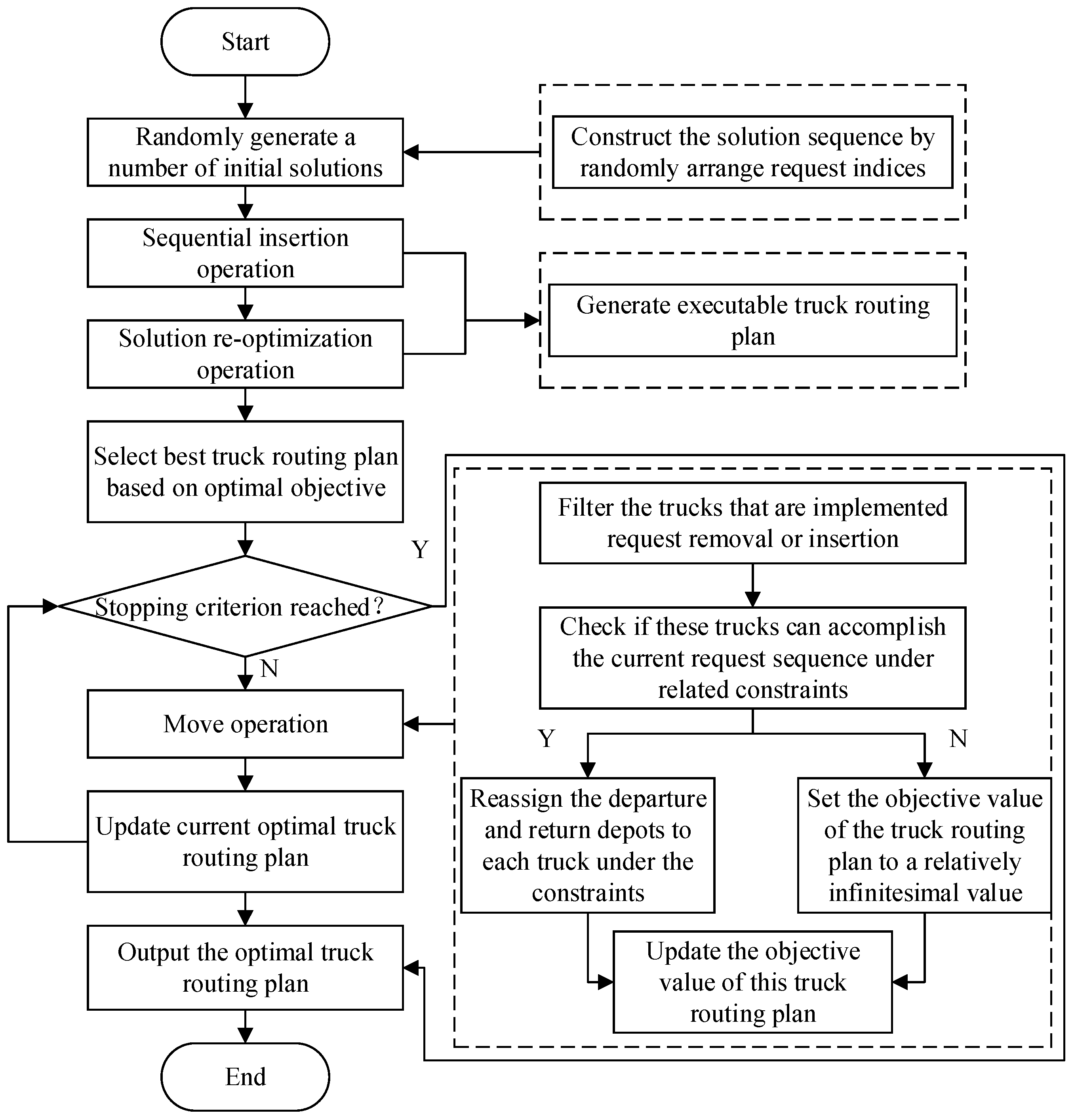
4. Solution Algorithm

The problem addressed in this study is NP-hard, with the number of feasible solutions increasing exponentially as the problem size grows. The proposed MILP model can be solved with commercial software like Gurobi 10.0.2. However, it is only capable of solving modest-scale instances to optimality or sub-optimality. Given the challenge that industrial-scale instances require significant memory and extended computation time, an alternative approach, LNS, is proposed to solve the problem. LNS was initially proposed by Shaw [46] to solve the vehicle routing problem (VRP), and has been effectively applied to various VRP variants in recent years [47,48,49]. The core idea of LNS is to generate a large neighborhood in each iteration using a specific search strategy to explore the solution space and find better solutions. In this study, the move operation is used as the search strategy, where a random set of request vertices is selected based on the removal coefficient, removed from the current solution, and reinserted into different positions.
Although LNS is generally applicable to the VRP, it has shortcomings in terms of solution efficiency. To tackle this issue, we proposed two innovative methods—“Sequential insertion” and “Solution re-optimization”—to improve the LNS. The proposed LNS represents the solution as a sequence of request nodes arranged in order, employing a numerical encoding technique. However, it does not specify from which depot a truck is dispatched to serve which customers. Therefore, a “Sequential insertion” method is introduced to decode the solution into several truck routes by selecting an appropriate depot for insertion. Although this method can transform the solution into truck routes, there is still a high possibility of high truck waiting costs, and sometimes it may violate the empty container constraints and the service priority constraints for composite requests. In order to enhance the quality of the solution, a “Solution re-optimization” method is designed to adjust the truck’s visiting time at each vertex and evaluate whether the re-optimized truck routes satisfy the empty container constraints. Figure 2 illustrates the framework of the improved LNS algorithm, with a comprehensive explanation of the implementation steps provided thereafter.

4.1. Generation of Initial Solution

The comprehensive CDP proposed in our study incorporates complex constraints, such as the capacity of trucks, the number of empty containers at depots, the service time windows for requests, and the service priority of composite requests. Coupled with two trucking operation modes and two empty container repositioning strategies, this has rendered predicting the truck route length a challenging task. Traditional methods for generating an initial solution, e.g., randomly assigning requests to each truck may result in an abundance of infeasible solutions. Therefore, following Yang et al. [42], the initial solution of the LNS is constructed by randomly arranging the request indices, which are represented by real numbers, as shown in Figure 3a.
In order to convert the solution into an executable truck routing plan, the “Sequential insertion” and “Solution re-optimization” methods are implemented, considering factors such as the maximum working hours and capacity of trucks, service time windows for requests, service priority, forbidden arcs, and the maximum allowed number of departures and returns of trucks at each depot. However, generating only a single initial solution and using its corresponding truck routing plan as the current optimal solution does not guarantee feasibility. As a result, based on the problem scale, a certain number of initial solutions are randomly generated, and the truck routing plan with the optimal objective value is selected as the current optimal solution for subsequent move operations.

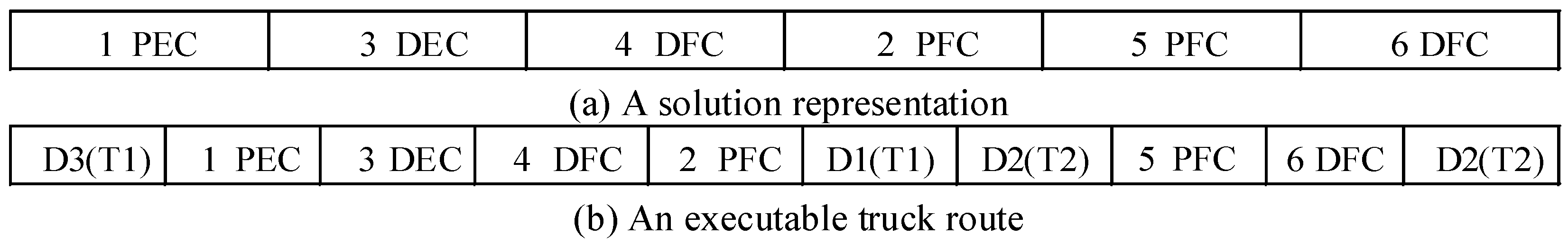
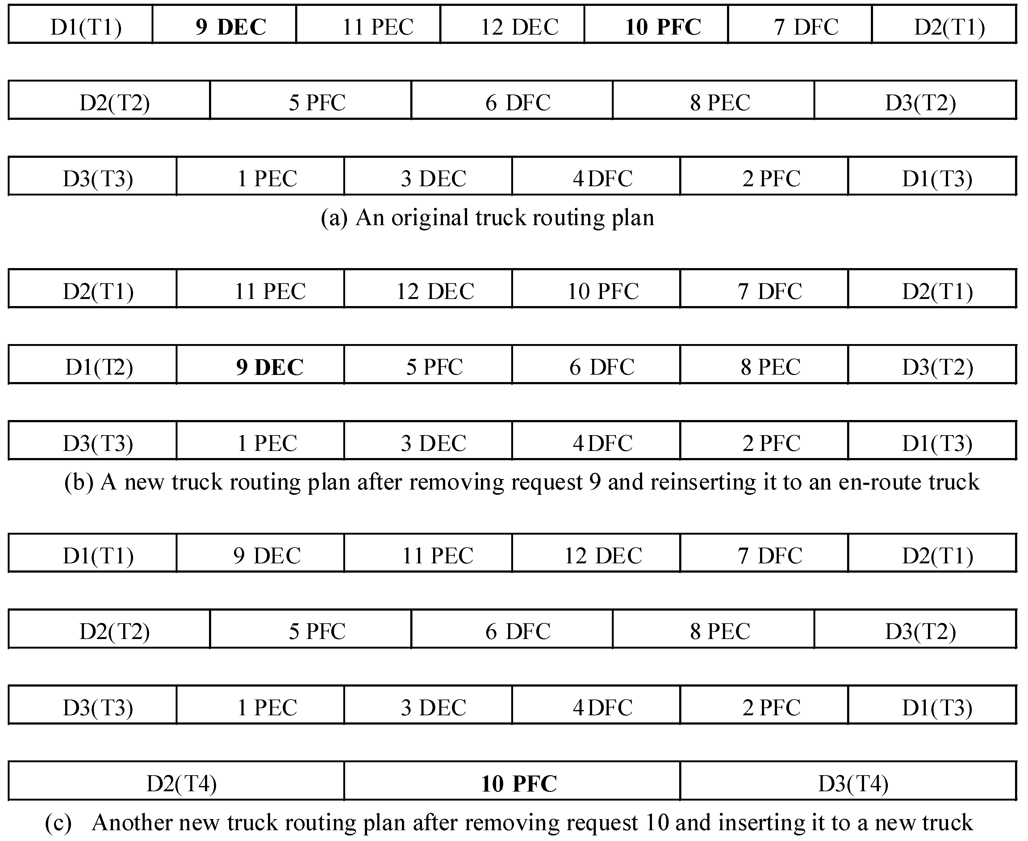
4.2. Sequential Insertion and Solution Re-Optimization Methods

Similarly to Yu et al. [11], the “Sequential insertion” method creates full truck routes by embedding depots within the ordered sequence of requests. The routes are subsequently improved using the “Solution re-optimization” method, as those generated by the “Sequential insertion” method may lack cost efficiency or even be infeasible in practice, potentially violating the empty container constraints at depots and the service priority constraints for composite requests.
Unlike Yu et al. [11], the “Sequential insertion” method, in addition to considering the truck’s operational time constraints and the service time windows for requests, also takes forbidden arcs into account when assessing whether the current truck can accommodate the present request. If the truck can accommodate the request, it is added sequentially to the truck’s service list. Temporal factors, such as the time required for the truck to traverse all request vertices, are subsequently adjusted according to the principle of minimizing total working time, which also considers the service time windows for all selected requests. The truck’s working time is then updated. This iterative process continues as the algorithm progresses through each subsequent request in the solution sequence. Once the current request violates the truck’s operational time constraints, the algorithm initiates a process to select the suitable depot for truck’s return. This selection process accounts for both the limit on truck return frequency and the nearest distance principle. Subsequently, a new truck will be dispatched to serve this request, and the “Sequential insertion” procedure restarts. In cases where the current request is the first to be served by a truck, a depot must be selected for truck dispatch, factoring in the limit on truck dispatch frequency and the nearest distance principle. Additionally, if the request requires the delivery of an empty container, the availability of empty containers is also taken into account. As shown in Figure 3a, the solution starts as a random arrangement of request indices. Depots are then added to divide it into sub-solutions, each representing a viable truck route, as illustrated in Figure 3b.
The “Solution re-optimization” method comprises two distinct steps. The first step focuses on refining the truck visiting time at each vertex, while maintaining the routes of all trucks unchanged. The primary goal of this step is to minimize the total working time of the trucks so as to improve the truck routes with high waiting costs produced by the “Sequential insertion” method. If the re-optimized truck routes fail to satisfy the service priority constraints for composite requests, they are deemed infeasible and the corresponding solution is discarded; otherwise, the second step is executed. The second step seeks to assess if the re-optimized feasible truck routes satisfy the empty container constraints at depots. It is important to note that when the truck performs two activities—delivering empty containers to the depots and picking them up from the depots—the number of empty containers at each depot changes dynamically. These activities correspond to transportation requests involving the delivery and pickup of empty containers, where the depot may serve as either the origin or destination. In the “Sequential insertion” operation, the depots are inserted into the solution based on the sequence of request vertices, and the number of empty containers at each depot fluctuates according to the sequence in which trucks are assigned to perform these two activities. However, in practice, the number of empty containers at each depot should dynamically change based on the specific timing of the aforementioned two activities. Consequently, the re-optimization process will derive the detailed delivery and pickup times for empty containers by trucks at each depot, utilizing the outcome from the first step. It will subsequently perform a dynamic calculation of the empty container quantities at each depot. If the empty container quantity at any depot is negative, the solution is deemed infeasible; otherwise, an executable truck routing plan is obtained.

4.3. Move Operation

In the proposed LNS, the move operation is chosen as the neighborhood search strategy and is applied to the optimal truck routing plan obtained after the “Sequential insertion” and “Solution re-optimization” operations. A certain number of request vertices are randomly selected based on the removal coefficient to undergo move operations. These request vertices are then sequentially removed from the current truck routing plan and reinserted into different positions. Specifically, for each request vertex to be inserted, any position within the current truck routing plan that complies with network flow constraints can be selected for insertion. When a request vertex is inserted into a specific position in the current routing plan, it is necessary to re-select the departure and return depots for each truck according to the nearest distance principle, under the constraints of the number of departures and returns of trucks at the depots and the empty container quantity at the depots. A new truck routing plan can be efficiently generated through this process.
For the newly generated truck routing plan, it is necessary to check whether each truck meets the constraints of maximum working hours, request service time windows, and forbidden arcs. Additionally, the empty container quantity at each depot must be dynamically evaluated to ensure it is greater than zero, based on the specific time of empty container delivery to and pickup from each depot. If the new routing plan fails to satisfy all constraints, it is considered infeasible. Conversely, if it meets all constraints and has a better objective value than the current optimal solution, it is updated as the current optimal solution.
Figure 4 illustrates two simple cases of move operations. The original truck routing plan (Figure 4a) employs three trucks while satisfying a series of constraints, including the truck’s working time limit, capacity, request time windows, forbidden arcs, service priority, the number of departures and returns of trucks at depots, and the quantity of empty containers at each depot. By removing the first request vertex in the service sequence of the first truck (request 9) and inserting it into the first position of the service sequence of the second truck, a new truck routing plan (Figure 4b) can be generated. This new plan uses the same number of trucks, but the departure depots for the first and second trucks are modified due to the change in their first service vertex. Additionally, by removing the fourth request vertex of the service sequence of the first truck (request 10) and inserting it into the first position of the service sequence of a newly introduced fourth truck, another new routing plan (Figure 4c) is formed. In this case, the number of trucks increases by one, while the departure and return depots for the first, second, and third trucks remain unchanged.

4.4. Stopping Criterion

The LNS iterates until a predefined stopping criterion is met. In this study, the stopping criterion is defined by the maximum number of iterations. This parameter establishes an upper bound on the number of iterations the algorithm will undergo before termination. For instances of varying scales, different iteration limits may be applied to attain optimal convergence. The iteration count is incremented by one once all selected request vertices have completed their move operations.

5. Numerical Experiments

In this section, we validate and evaluate the proposed MILP model and the improved LNS algorithm through extensive numerical experiments. All the experiments are carried out on a personal computer (Intel Xeon W-2775 Processor @3.30 GHz with 64 GB of RAM). The linearized MILP model is coded in Gurobi 10.0.2. The LNS is implemented in Matlab R2022a using the C++ language.

5.1. Experiments Setting and Instances Generation

Since the proposed comprehensive CDP encompasses eight types of requests, no publicly available benchmark instances can be found in the literature. Therefore, the experimental instances are generated randomly, using a method similar to those applied in prior studies, such as Zhang et al. [10] and Yu et al. [11]. For each instance, the locations of a container terminal, six inland depots, and a certain number of customers (shippers and consignees) are stochastically distributed on a Euclidean plane, with both the length and width corresponding to a 3 h distance by truck. It is important to highlight that the terminal fulfills two distinct functions in this context. For the IF and OF requests, the terminal is considered a bypass node, and its function is solely to calculate the transfer time on the arc passing through the terminal. In contrast, for the IE and OE requests by shipping companies, their locations are actually the terminal. However, in the vertex configuration, these locations are assigned distinct numerical identifiers, despite having identical coordinates. The time needed for loading (or unloading) a container onto (or from) a truck is 0.1 h, while the time required for packing or unpacking a container is 0.4 h. Additionally, the left boundary of the request time window is randomly assigned within a range of [0, 4] h, with the width of the time window varying between 4 and 8 h.
The traveling speed of a truck is assumed to be constant, irrespective of whether it is loaded or empty. The cost parameters C 1 , C 2 , and C 3 are set to 6.516, 1744, and 56.295, respectively, based on the values reported by He et al. [50] and Yang et al. [42]. It should be noted that C 1 is only the total fuel cost and carbon emissions cost per unit of traveling time, which does not include the fixed one-time startup cost of dispatching a truck for a request. The parameters of the LNS algorithm, including the number of initial solutions, maximum number of iterations, and removal coefficient, are tailored to the specific characteristics of each instance under consideration. The scope of the removal coefficient ranges from 0.2 to 0.8. To ensure the results’ reliability, each experimental instance was solved multiple times with the LNS, which may vary depending on the problem size, thus reducing the impact of randomness.
In practical scenarios, a random combination of diverse request types may arise. To assess the performance of the proposed LNS, fifty experimental instances of varying sizes, spanning small-, medium-, large-, and super-large-scale instances, are generated. These instances are characterized by the quantities of each request type and the number of empty containers at each depot. Taking instance 6 as an example, the column “No. of Requests” indicates that the total number of requests is 12, with the distribution of eight request types (IF, ER, ED, OF, IE, OE, IFER, and OFED) as follows: 1, 1, 2, 0, 1, 2, 2, and 3, respectively. Additionally, the column “No. of Empty Containers” shows that the number of empty containers at depots 1 through 6 is 1, 0, 0, 2, 1, and 0, respectively. However, it is common for some customers to require trucks to remain at their locations awaiting packing or unpacking when handling composite requests. This necessitates the use of the Stay-with mode and adds complexity to the scheduling of trucks. Such customers are included in some of the super-large-scale instances. For example, in instance 42, “40 (10)” indicates that there are 40 customers with IFER requests, of which 10 need trucks to wait for packing or unpacking.

5.2. Experiments on Small- and Medium-Scale Instances

To validate the correctness of the proposed MILP model for the comprehensive CDP, as well as evaluate the performance of the LNS, ten small-scale instances and ten medium–scale instances are generated. All the instances are solved using both Gurobi and the LNS. The results of objective values and solving time are reported in Table 4 and Table 5, respectively.
Firstly, as presented in Table 4 and Table 5, the results obtained from the small-scale and medium-scale instances provide strong evidence supporting the validity of the model. For all the small-scale instances, Gurobi is able to find the optimal solutions with an average solving time of 260 s and a maximum solving time of 729 s. As the instance scale increases, the solving time rises significantly. It is important to note that the complexity of the problem depends not only on the total number of requests but also on the number of composite requests. In short, it is determined by the total number of request vertices after decomposing the composite requests. Therefore, although instances 10 and 11 have the same number of requests, the split of composite requests substantially increases the computational burden, leading to Gurobi being unable to find the optimal solutions for instance 11 and other medium-scale instances within 1 h. However, the average gap between the objective value and the lower bound across the ten medium-scale instances is only 4.81%, demonstrating that Gurobi is capable of providing near-optimal solutions. Such a level of performance exhibited by the MILP model can be regarded as acceptable for practical scenarios.
Secondly, Table 4 and Table 5 also validate the outstanding performance of the proposed LNS. In particular, the LNS is able to optimally solve instances 1 to 5 in an average time of just 2.74 s, significantly faster than Gurobi, which takes an average of 49.60 s. For the remaining five small-scale instances and some medium-scale instances (11, 12, 13, 16, and 19), although the LNS yields slightly higher objective values than Gurobi, the average gap is only 2.88%. The reason why the solutions obtained by LNS are worse than those from Gurobi can be attributed to two factors. One factor is that LNS may become trapped in local optima. Another factor is that the “sequential insertion” operation proposed in this study is a heuristic method. It converts the solution sequence into a truck routing plan according to specific rules while ensuring feasibility. However, even if the solution sequence originates from an optimal truck routing plan, this approach does not guarantee the generation of an optimal solution. Although this limitation exists, the advantage of the LNS becomes more pronounced as the scale of the instances increases, both in terms of objective values and solving time. The LNS can solve instances 14, 15, 17, 18, and 20 within an average time of only 44.07 s, while it also provides better solutions than Gurobi within a 1 h time limit. For all the small-scale and medium-scale instances, the gap between the LNS and Gurobi is only 0.26%, while the LNS requires considerably less solving time, further validating its effectiveness and its potential for larger scale instances.

5.3. Experiments on Large- and Super-Large-Scale Instances

The NP-hard nature of the MILP model makes obtaining optimal solutions for larger-scale instances impractical, with even finding a feasible solution for such instances proving to be challenging. In order to further investigate the performance of the LNS on large-scale and super-large-scale instances, the results are compared with the GA proposed by Yu et al. [11]. Since their study does not include forbidden arcs for IE and OE request vertices, the GA is then tailored to accommodate these constraints. As described in Wang and Regan [4], a sub-fleet can handle a maximum of 75 transport requests per day. Consequently, in this section, twenty large-scale instances are randomly generated, with the maximum number of requests set at 75 before the request vertex split and 135 after the split. Additionally, ten super-large-scale instances are generated, featuring transport request counts ranging from 100 to 480, with the total number of requests after vertex split ranging from 160 to 760. The results are shown in Table 6 and Table 7.
From Table 6 and Table 7, it can be observed that as the problem size increases, both the LNS and GA algorithms exhibit similar increase trends in terms of objective values and solution time, which proves the stability of the algorithms. Although there appears to be some fluctuation, the objective values and solution time are closely related to the number of request vertices after the split. To illustrate, while the number of requests in instances 23 and 24 is the same, instance 24 has more composite requests, which results in a greater number of request vertices, thus leading to higher costs and longer solution time compared to instance 23.
Notably, the proposed LNS obviously outperforms GA in terms of both the objective values and solution time for large-scale and super-large-scale instances. When the total number of transport requests after vertex split does not exceed 135, both the LNS and GA are able to find solutions with excellent convergence within 126 s. However, on average, the LNS is 4.47 s faster than GA, and its objective values are 3.53% lower than those of GA. On the other hand, when the total number of transport requests after vertex split exceeds 160, the solving time of both LNS and GA shows a sharp increase. This phenomenon indicates that the problem size has a significant impact on the performance of the algorithms, especially in terms of solution complexity and computational resource requirements. The advantage of LNS becomes particularly evident for super-large-scale instances, where it has an average solving time of 107.78 s shorter than GA and an average objective value 3.86% lower than that of GA. Additionally, LNS has the capacity to yield solutions with relatively acceptable convergence within 3550 s for all the super-large-scale instances. All in all, the proposed LNS demonstrates a clear advantage by consistently providing significantly better solutions compared to the algorithm of Yu et al. [11], all while requiring much less computational time. This not only highlights the effectiveness and efficiency of the LNS but also serves as strong validation for its performance, reinforcing its potential as a more optimal approach in solving the problem at hand.

5.4. Stability Analysis of the LNS

To assess the stability of the LNS algorithm, this section first analyzes the smoothness of the convergence curve for LNS by comparing it with that for GA, and then evaluates the consistency of the results across multiple experiments conducted on different instances.
The convergence curves for both LNS and GA are obtained using instances 45 and 50, as illustrated in Figure 5. The results clearly indicate a distinct advantage of LNS in the optimization process. The convergence curve of LNS is significantly smoother and exhibits a faster rate of descent compared to GA, particularly during the early stages. The LNS is able to quickly identify relatively optimal solutions and sustain a faster optimization rate in subsequent stages. In contrast, the GA convergence curve displays greater volatility, with a slower descent rate, typically requiring more generations to achieve meaningful improvements in the objective function. This suggests that the LNS possesses superior local search capabilities in the short term, allowing it to rapidly converge to better solutions, whereas the GA may become trapped in larger fluctuations within the search space, thus requiring more time for fine-tuning the solution. In later stages, the convergence curve of LNS stabilizes, with convergence occurring at approximately 160 iterations for instances 45 and 340 iterations for instance 50, demonstrating that the optimization process has reached stability and the objective value is approaching a local or global optimum. Conversely, the GA curve may exhibit oscillations, indicating that the algorithm is still exploring the solution space and has not yet reached a stable state. In conclusion, Figure 5 not only demonstrates that the LNS can achieve convergence during the iteration process, but also shows that the number of iterations required for convergence increases as the instance size grows.
Furthermore, the consistency of the results obtained by LNS is examined using instances selected from large-scale and super-large-scale problems, as shown in Table 8. Each instance is run ten times. The first column lists the instance index, while the second and third columns show the minimum and maximum objective values from the ten runs. The fourth column presents the average objective value, and the final column displays the difference between the maximum and minimum values. The largest difference is 0.41%, while the average difference is only 0.27%, indicating that the optimal solution experiences minimal fluctuations, thereby demonstrating the stability of LNS.

5.5. Sensitivity Analysis

Intuitively, the costs of the CDP are influenced not only by the number of depots and empty containers, but also by their distribution across multiple depots. In a container drayage system, inland depots are typically located at integrated logistics parks or near industrial clusters or consumer markets to reduce transport costs. However, it is impractical to build a depot for each of them, nor can an infinite supply of empty containers be provided. In order to offer practical recommendations from a decision-support perspective, this section first analyzes the impact of depot and empty container numbers on the total transport costs, followed by the effect of depot distribution and empty container distribution across depots.

5.5.1. Effect of the Number of Depots and Empty Containers

Due to the random generation of depot and customer locations, the results of a single experiment exhibit a high degree of uncertainty. To reduce the impact of this uncertainty, for each selected instance, 10 experimental scenarios with varying request vertices are randomly generated while ensuring that the total number of requests is fixed. Notably, the locations of depots are also randomly distributed, but remain fixed for the 10 experimental scenarios. The results for instances 38 and 46 are each presented in an individual 3D surface plot, as shown in Figure 6.
It is important to note that as the number of depots increases, the benefit of providing an adequate supply of empty containers initially becomes evident. However, when the number of depots reaches a sufficiently high level, the marginal impact of further increasing the number of empty containers on the objective value diminishes. Under the same number of empty containers, increasing the number of depots can significantly reduce the optimal objective value. However, once the number of depots reaches a certain threshold, e.g., five depots when there are 13 empty containers in Figure 6a, its effect on the objective value gradually diminishes. This result indicates that an increase in the number of depots can lead to a more decentralized transport network, which may enhance the flexibility and the efficiency of truck dispatching and empty container repositioning, thereby reducing the total transportation costs. Furthermore, under the same number of depots, the more empty containers that can be supplied, the more options for truck dispatching become available, thereby helping to reduce the objective value. These observations highlight the importance of both depot placement and empty container availability in optimizing transportation networks, suggesting that an optimal balance between the number of depots and empty containers is crucial for minimizing transportation costs.

5.5.2. Effect of the Distribution of Depots and Empty Containers

It is worth pointing out that while the number of depots and empty containers is vital for a cost-effective container drayage system, their distribution is equally important and should also be considered. In the preceding sections, depots are randomly placed on a Euclidean plane. Additionally, multiple depots can be uniformly distributed within a specified area, or strategically placed in several key areas, depending on the transportation demand. These three distribution types are referred to as random, uniform, and focused distribution, respectively. Likewise, empty containers can be allocated across multiple depots using the same three distribution strategies. Specifically, the focused distribution of empty containers involves allocating more containers to depots situated within or near key areas. In this section, three combinations of distribution strategies—R/R, U/U, and F/F—are investigated with the results presented in Table 9. For example, F/F distribution means that both the distribution of depots and empty containers are focused within a defined area.
The results clearly indicate that as the number of empty container-related requests increases, the cost savings become greater. The average cost saving of the selected six instances under the U/U and F/F distribution from the R/R distribution is, respectively, 3.02% and 8.46%, demonstrating that both the U/U and F/F distribution outperforms the R/R distribution. This finding suggests that, under random request distribution, uniformly distributed depots and containers help maintain a relatively balanced service area and empty container transportation volume for each depot, reducing situations of excessively long transport distances and preventing the over-concentration or over-dispersion of empty container transportation. In contrast, focused distribution of depots and empty containers helps reduce the transport distance of large quantities of empty containers between depots and request vertices, as well as the distance for empty trucks departing from or returning to the depots, thereby more effectively reducing total transport costs.

6. Conclusions

In this paper, we address a comprehensive CDP that integrates eight types of common transportation requests, the availability of empty containers across multiple depots, the Stay-with and Drop-and-pull modes for handling composite requests, and the Depot-turn and Street-turn strategies for repositioning empty containers. A novel MILP model based on the DAOV graph is proposed to minimize the costs associated with fuel consumption, carbon emissions, and truck waiting times, while simultaneously optimizing decisions regarding empty container allocation, truck dispatching, and route planning. Due to the proposed MILP only solving small-scale instances optimally with Gurobi, an improved LNS algorithm, incorporating the “Sequential insertion” and the “Solution re-optimization” methods, has been developed to handle industrial-sized instances. The “Sequential insertion” method is responsible for converting the solution into multiple truck routes, while the “Solution re-optimization” method is used to refine the quality of solutions and ensure the feasibility of the truck routing plan.
The performance of the proposed algorithm has been validated by extensive experiments with varying scales. While Gurobi can solve the MILP model to optimality for small-scale instances, it can only obtain a near-optimal solution for medium-scale instances within 1 h. Although the average objective value of the LNS for all small-scale and medium-scale instances is 0.26% higher than that of the MILP, it consumes significantly less solving time. Additionally, LNS obviously outperforms GA in terms of both the objective values and solution time for large-scale and super-large-scale instances. In particular, the LNS has an average solving time that is 107.78 s shorter than GA, along with an average objective value 3.86% lower than that of GA for super-large-scale instances. The stability analysis of LNS and GA also demonstrates its ability to provide stable solutions for the proposed CDP.
Sensitivity analysis reveals the speculation that the number of depots and empty containers is a key factor in optimizing the container transportation network. However, as the number of depots or empty containers increases, the marginal impact on the total cost first rises and then diminishes. These findings indicate that achieving an optimal balance between depots and empty containers is essential for minimizing transportation costs. Furthermore, the uniform and focused distribution of depots and empty containers can reduce, respectively, 3.02% and 8.46% of the average total cost, as they help reduce the transport distance for large quantities of empty containers between depots and customers, as well as the distance for empty trucks departing from or returning to the depots.
Note that this study does not address the costs of depot construction and empty container purchases associated with their quantities, which could impact the payback period and operational efficiency, and should be determined from a planning perspective. It is worthwhile to investigate these factors when planning an efficient drayage system. Additionally, with the development of e-commerce drayage platforms, dynamic orders will gradually become an indispensable element, which poses a challenge to the online optimization of the comprehensive CDP.

Author Contributions

Conceptualization, X.Y.; methodology, X.Y.; software, C.H.; validation, X.Y. and C.H.; formal analysis, X.Y. and C.H.; investigation, X.Y.; resources, X.Y.; data curation, X.Y. and C.H.; writing—original draft preparation, X.Y.; writing—review and editing, X.Y.; visualization, C.H.; supervision, X.Y.; project administration, X.Y.; funding acquisition, X.Y. All authors have read and agreed to the published version of the manuscript.

Funding

This research was funded by the National Natural Science Foundation of China, grant number 42001122.

Institutional Review Board Statement

Not applicable.

Informed Consent Statement

Not applicable.

Data Availability Statement

The data presented in this study are available on request from the corresponding author.

Conflicts of Interest

The authors declare no conflicts of interest.

References

  1. Li, S.; Wu, W.; Ma, X.; Zhong, M.; Safdar, M. Modelling Medium- and Long-Term Purchasing Plans for Environment-Orientated Container Trucks: A Case Study of Yangtze River Port. Transp. Saf. Environ. 2023, 5, tdac043. [Google Scholar] [CrossRef]
  2. Cui, H.; Chen, S.; Chen, R.; Meng, Q. A Two-Stage Hybrid Heuristic Solution for the Container Drayage Problem with Trailer Reposition. Eur. J. Oper. Res. 2022, 299, 468–482. [Google Scholar] [CrossRef]
  3. Lee, S.; Moon, I. Robust Empty Container Repositioning Considering Foldable Containers. Eur. J. Oper. Res. 2020, 280, 909–925. [Google Scholar] [CrossRef]
  4. Wang, X.; Regan, A.C. Local Truckload Pickup and Delivery with Hard Time Window Constraints. Transp. Res. B Methodol. 2002, 36, 97–112. [Google Scholar] [CrossRef]
  5. Moghaddam, M.; Pearce, R.H.; Mokhtar, H.; Prato, C.G. A Generalised Model for Container Drayage Operations with Heterogeneous Fleet, Multi-Container Sizes and Two Modes of Operation. Transp. Res. E Logist. Transp. Rev. 2020, 139, 101973. [Google Scholar] [CrossRef]
  6. Song, Y.; Zhang, J.; Liang, Z.; Ye, C. An Exact Algorithm for the Container Drayage Problem under a Separation Mode. Transp. Res. E Logist. Transp. Rev. 2017, 106, 231–254. [Google Scholar] [CrossRef]
  7. Imai, A.; Nishimura, E.; Current, J. A Lagrangian Relaxation-Based Heuristic for the Vehicle Routing with Full Container Load. Eur. J. Oper. Res. 2007, 176, 87–105. [Google Scholar] [CrossRef]
  8. Chen, R.; Meng, Q.; Jia, P. Container Port Drayage Operations and Management: Past and Future. Transp. Res. E: Logist. Transp. Rev. 2022, 159, 102633. [Google Scholar] [CrossRef]
  9. Song, Y.; Zhang, Y. A Branch-and-Price-and-Cut Algorithm for the Inland Container Transportation Problem with Limited Depot Capacity. Appl. Sci. 2024, 14, 11958. [Google Scholar] [CrossRef]
  10. Zhang, R.; Huang, C.; Wang, J. A Novel Mathematical Model and a Large Neighborhood Search Algorithm for Container Drayage Operations with Multi-Resource Constraints. Comput. Ind. Eng. 2020, 139, 106143. [Google Scholar] [CrossRef]
  11. Yu, X.; Feng, Y.; He, C.; Liu, C. Modeling and Optimization of Container Drayage Problem with Empty Container Constraints across Multiple Inland Depots. Sustainability 2024, 16, 5090. [Google Scholar] [CrossRef]
  12. Fazi, S.; Choudhary, S.K.; Dong, J.-X. The Multi-Trip Container Drayage Problem with Synchronization for Efficient Empty Containers Re-Usage. Eur. J. Oper. Res. 2023, 310, 343–359. [Google Scholar] [CrossRef]
  13. Jula, H.; Dessouky, M.; Ioannou, P.; Chassiakos, A. Container Movement by Trucks in Metropolitan Networks: Modeling and Optimization. Transp. Res. E Logist. Transp. Rev. 2005, 41, 235–259. [Google Scholar] [CrossRef]
  14. Chung, K.H.; Ko, C.S.; Shin, J.Y.; Hwang, H.; Kim, K.H. Development of Mathematical Models for the Container Road Transportation in Korean Trucking Industries. Comput. Ind. Eng. 2007, 53, 252–262. [Google Scholar] [CrossRef]
  15. Vidović, M.; Popović, D.; Ratković, B.; Radivojević, G. Generalized Mixed Integer and VNS Heuristic Approach to Solving the Multisize Containers Drayage Problem. Int. Trans. Oper. Res. 2017, 24, 583–614. [Google Scholar] [CrossRef]
  16. Yang, X.; Daham, H.A. A Column Generation-Based Decomposition and Aggregation Approach for Combining Orders in Inland Transportation of Containers. OR Spectr. 2020, 42, 261–296. [Google Scholar] [CrossRef]
  17. Bruglieri, M.; Mancini, S.; Peruzzini, R.; Pisacane, O. The Multi-Period Multi-Trip Container Drayage Problem with Release and Due Dates. Comput. Oper. Res. 2021, 125, 105102. [Google Scholar] [CrossRef]
  18. Bjelić, N.; Vidović, M.; Popović, D.; Ratković, B. Rolling-Horizon Approach in Solving Dynamic Multisize Multi-Trailer Container Drayage Problem. Expert. Syst. Appl. 2022, 201, 117170. [Google Scholar] [CrossRef]
  19. Jia, S.; Cui, H.; Chen, R.; Meng, Q. Dynamic Container Drayage with Uncertain Request Arrival Times and Service Time Windows. Transp. Res. B Methodol. 2022, 166, 237–258. [Google Scholar] [CrossRef]
  20. Chen, R.; Jia, S.; Meng, Q. Dynamic Container Drayage Booking and Routing Decision Support Approach for E-Commerce Platforms. Transp. Res. E Logist. Transp. Rev. 2023, 177, 103220. [Google Scholar] [CrossRef]
  21. Ran, C.; Zhang, Y. The Driving Force of Carbon Emissions Reduction in China: Does Green Finance Work. J. Clean. Prod. 2023, 421, 138502. [Google Scholar] [CrossRef]
  22. Xiao, L.; Chen, L.; Sun, P.; Laporte, G.; Baldacci, R. The Container Drayage Problem for Electric Trucks with Charging Resource Constraints. Transp. Res. C Emerg. Technol. 2025, 174, 105100. [Google Scholar] [CrossRef]
  23. Caris, A.; Janssens, G.K. A Local Search Heuristic for the Pre- and End-Haulage of Intermodal Container Terminals. Comput. Oper. Res. 2009, 36, 2763–2772. [Google Scholar] [CrossRef]
  24. Lai, M.; Crainic, T.G.; Di Francesco, M.; Zuddas, P. An Heuristic Search for the Routing of Heterogeneous Trucks with Single and Double Container Loads. Transp. Res. E Logist. Transp. Rev. 2013, 56, 108–118. [Google Scholar] [CrossRef]
  25. Ghezelsoflu, A.; Di Francesco, M.; Frangioni, A.; Zuddas, P. A Set-Covering Formulation for a Drayage Problem with Single and Double Container Loads. J. Ind. Eng. Int. 2018, 14, 665–676. [Google Scholar] [CrossRef]
  26. Xue, Z.; Zhang, C.; Lin, W.-H.; Miao, L.; Yang, P. A Tabu Search Heuristic for the Local Container Drayage Problem under a New Operation Mode. Transp. Res. E Logist. Transp. Rev. 2014, 62, 136–150. [Google Scholar] [CrossRef]
  27. Wang, D.; Moon, I.; Zhang, R. Multi-Trip Multi-Trailer Drop-and-Pull Container Drayage Problem. IEEE Trans. Intell. Transp. Syst. 2022, 23, 19088–19104. [Google Scholar] [CrossRef]
  28. Wang, N.; Meng, Q.; Zhang, C. A Branch-Price-and-Cut Algorithm for the Local Container Drayage Problem with Controllable Vehicle Interference. Transp. Res. B Methodol. 2023, 178, 102835. [Google Scholar] [CrossRef]
  29. You, J.; Miao, L.; Zhang, C.; Xue, Z. A Generic Model for the Local Container Drayage Problem Using the Emerging Truck Platooning Operation Mode. Transp. Res. B Methodol. 2020, 133, 181–209. [Google Scholar] [CrossRef]
  30. Xue, Z.; Lin, H.; You, J. Local Container Drayage Problem with Truck Platooning Mode. Transp. Res. E Logist. Transp. Rev. 2021, 147, 102211. [Google Scholar] [CrossRef]
  31. Yan, X.; Xu, M.; Xie, C. Local Container Drayage Problem with Improved Truck Platooning Operations. Transp. Res. E Logist. Transp. Rev. 2023, 169, 102992. [Google Scholar] [CrossRef]
  32. You, J.; Wang, Y.; Xue, Z. An Exact Algorithm for the Multi-Trip Container Drayage Problem with Truck Platooning. Transp. Res. E Logist. Transp. Rev. 2023, 175, 103138. [Google Scholar] [CrossRef]
  33. Huang, Y.; Jin, Z.; Liu, P.; Wang, W.; Zhang, D. Container Drayage Problem Integrated with Truck Appointment System and Separation Mode. Comput. Ind. Eng. 2024, 193, 110307. [Google Scholar] [CrossRef]
  34. Wang, D.; Zhang, R.; Dong, M.; Xie, X. Drop-and-Pull Container Drayage with Route Balancing and Its Matheuristic Algorithm. Expert Syst. Appl. 2024, 255, 124625. [Google Scholar] [CrossRef]
  35. Zhang, R.; Yun, W.Y.; Moon, I. A Reactive Tabu Search Algorithm for the Multi-Depot Container Truck Transportation Problem. Transp. Res. E Logist. Transp. Rev. 2009, 45, 904–914. [Google Scholar] [CrossRef]
  36. Zhang, R.; Yun, W.Y.; Kopfer, H. Heuristic-Based Truck Scheduling for Inland Container Transportation. OR Spectr. 2010, 32, 787–808. [Google Scholar] [CrossRef]
  37. Nossack, J.; Pesch, E. A Truck Scheduling Problem Arising in Intermodal Container Transportation. Eur. J. Oper. Res. 2013, 230, 666–680. [Google Scholar] [CrossRef]
  38. Sterzik, S.; Kopfer, H. A Tabu Search Heuristic for the Inland Container Transportation Problem. Comput. Oper. Res. 2013, 40, 953–962. [Google Scholar] [CrossRef]
  39. Braekers, K.; Caris, A.; Janssens, G.K. Integrated Planning of Loaded and Empty Container Movements. OR Spectr. 2013, 35, 457–478. [Google Scholar] [CrossRef]
  40. Zhang, R.; Yun, W.Y.; Kopfer, H. Multi-Size Container Transportation by Truck: Modeling and Optimization. Flex. Serv. Manuf. J. 2015, 27, 403–430. [Google Scholar] [CrossRef]
  41. Funke, J.; Kopfer, H. A Model for a Multi-Size Inland Container Transportation Problem. Transp. Res. E Logist. Transp. Rev. 2016, 89, 70–85. [Google Scholar] [CrossRef]
  42. Yang, X.; Daham, H.A.; Salhi, A. Combined Strip and Discharge Delivery of Containers in Heterogeneous Fleets with Time Windows. Comput. Oper. Res. 2021, 127, 105141. [Google Scholar] [CrossRef]
  43. Zhang, R.; Yun, W.Y.; Moon, I.K. Modeling and Optimization of a Container Drayage Problem with Resource Constraints. Int. J. Prod. Econ. 2011, 133, 351–359. [Google Scholar] [CrossRef]
  44. Song, Y.; Zhang, Y.; Wang, W.; Xue, M. A Branch and Price Algorithm for the Drop-and-Pickup Container Drayage Problem with Empty Container Constraints. Sustainability 2023, 15, 5638. [Google Scholar] [CrossRef]
  45. Huang, C.; Zhang, R. Container Drayage Transportation Scheduling With Foldable and Standard Containers. IEEE Trans. Eng. Manage 2023, 70, 3497–3511. [Google Scholar] [CrossRef]
  46. Shaw, P. Using Constraint Programming and Local Search Methods to Solve Vehicle Routing Problems. In Principles and Practice of Constraint Programming—CP98; Maher, M., Puget, J.-F., Eds.; Lecture Notes in Computer Science; Springer: Berlin/Heidelberg, Germany, 1998; Volume 1520, pp. 417–431. ISBN 978-3-540-65224-3. [Google Scholar]
  47. Hintsch, T.; Irnich, S. Large Multiple Neighborhood Search for the Clustered Vehicle-Routing Problem. Eur. J. Oper. Res. 2018, 270, 118–131. [Google Scholar] [CrossRef]
  48. Hojabri, H.; Gendreau, M.; Potvin, J.-Y.; Rousseau, L.-M. Large Neighborhood Search with Constraint Programming for a Vehicle Routing Problem with Synchronization Constraints. Comput. Oper. Res. 2018, 92, 87–97. [Google Scholar] [CrossRef]
  49. Bustos-Coral, D.; Costa, A.M. Adaptive Large Neighborhood Search for Drayage Routing Problems Involving Longer Combination Vehicles. Comput. Oper. Res. 2025, 173, 106826. [Google Scholar] [CrossRef]
  50. He, W.; Jin, Z.; Huang, Y.; Xu, S. The Inland Container Transportation Problem with Separation Mode Considering Carbon Dioxide Emissions. Sustainability 2021, 13, 1573. [Google Scholar] [CrossRef]
Figure 1. Illustration of the eight types of transport requests.
Applsci 15 05937 g001
Figure 2. Framework of the improved LNS algorithm.
Applsci 15 05937 g002
Figure 3. A sample of an initial solution and the executable truck route after applying Sequential insertion operation.
Applsci 15 05937 g003
Figure 4. Move operations.
Applsci 15 05937 g004
Figure 5. Convergence curves of the LNS and GA.
Applsci 15 05937 g005
Figure 6. Effect of the number of depots and the number of empty containers.
Applsci 15 05937 g006
Table 1. Comparative summary of related articles.
ArticleRequest TypeOperation ModesEmpty StrategiesFeatureMethodology
S.W.D.P.D.S.S.S.m-depotEmptyExactHeuristic
Imai et al. [7]7, 8×××××
Caris and Janssens [23]7, 8×××××
Lai et al. [24]7, 8×××××
Ghezelsoflu et al. [25]7, 8×××××
Xue et al. [26]7, 8×××××
Cui et al. [2]7, 8×××××
Wang et al. [27]7, 8××××××
Wang et al. [28]7, 8××××
You et al. [29]7, 8×××
Xue et al. [30]7, 8×××
Yan et al. [31]7, 8×××
You et al. [32]7, 8××××
Huang et al. [33]7, 8×××
Wang et al. [34]7, 8××××
Zhang et al. [35]5, 6, 7, 8×××
Zhang et al. [36]5, 6, 7, 8×××
Nossack and Pesch [37]5, 6, 7, 8×××
Sterzik and Kopfer [38]5, 6, 7, 8××
Braekers et al. [39]5, 6, 7, 8×××
Zhang et al. [40]5, 6, 7, 8××××
Zhang et al. [10]5, 6, 7, 8×××
Funke and Kopfer [41]5, 6, 7, 8×××
Yang et al. [42]5, 6, 7, 8×
Zhang et al. [43]5, 7, 8××
Song et al. [6]6, 7, 8××××
Song et al. [44]6, 7, 8×××
Huang and Zhang [45]6, 7, 8××
Fazi et al. [12]1, 3, 4, 7, 8××
Moghaddam et al. [5]1, 2, 3, 4, 7, 8××
Yu et al. [11]1, 2, 3, 4, 7, 8
1: IF; 2: ER; 3: ED; 4: OF; 5: IE; 6: OE; 7: IFER; 8: OFED; S.W.: Stay-with mode; D.P.: Drop-and-pull mode; D.S.: Depot-turn strategy; S.S.: Street-turn strategy; m-depot: multiple depots; Empty.: empty container constraints.
Table 2. Activities at request vertices.
Request VerticesRequest TypesActivities at Request Vertices
N D E C ED, OEDelivering an empty container to either a customer or the terminal
N D F C IFDelivering a full container to a customer
N P E C ER, IEPicking up an empty container from either a customer or the terminal
N P F C OFPicking up a full container from a customer
Table 3. Activities and transfer time on arcs (i, j).
( i , j ) j N d j N D E C j N D F C j N P E C j N P F C
i N d /Picking up an empty container from the depot i and proceeding to vertex jProceeding to the terminal, picking up an import full container, and proceeding to the consignee jProceeding to vertex jProceeding to the shipper j
t i j t i 0 + t 0 + t 0 j t i j t i j
i N D E C Returning to the depot j/Proceeding to the terminal, picking up an import full container, and proceeding to the consignee jProceeding to vertex jProceeding to the shipper j
t i j t i 0 + t 0 + t 0 j t i j t i j
i N D F C Returning to the depot j/Proceeding to the terminal, picking up an import full container, and proceeding to the consignee jProceeding to vertex jProceeding to the shipper j
t i j t i 0 + t 0 + t 0 j t i j t i j
i N P E C Returning to the depot j and dropping off an empty containerProceeding to vertex j///
t i j t i j
i N P F C Proceeding to the terminal, dropping off an export full container, and returning to the depot j/Proceeding to the terminal to drop off an export full container, then picking up an import full container, and proceeding to the consignee jProceeding to the terminal, dropping off an export full container, and proceeding to vertex jProceeding to the terminal, dropping off an export full container, and proceeding to the shipper j
t i 0 + t 0 + t 0 j t i 0 + 2 t 0 + t 0 j t i 0 + t 0 + t 0 j t i 0 + t 0 + t 0 j
Table 4. Results of Gurobi and LNS for small-scale instances.
InstanceNo. of RequestsNo. of Empty ContainersCostTime (s)Gap
(%)
GurobiLNSGurobiLNS
15 (1, 0, 0, 1, 1, 1, 0, 1)(1, 0, 1, 0, 0, 0)89.889.8261.210.00
26 (1, 1, 0, 1, 0, 1, 1, 1)(1, 0, 1, 0, 0, 0)113.6113.6331.300.00
37 (0, 1, 1, 2, 1, 0, 0, 2)(1, 0, 1, 0, 0, 0)145.3145.3451.270.00
48 (1, 1, 0, 1, 1, 0, 0, 4)(1, 0, 1, 0, 0, 0)198.9198.9662.250.00
510 (2, 0, 0, 1, 0, 2, 3, 2)(1, 0, 1, 0, 0, 0)211.5211.5787.660.00
612 (1, 1, 2, 0, 1, 2, 2, 3)(1, 0, 0, 2, 1, 0)244.5246.319512.390.74
714 (1, 1, 3, 3, 1, 1, 2, 2)(0, 1, 1, 0, 0, 0)245.1248.821319.541.51
816 (3, 0, 1, 3, 1, 1, 2, 5)(0, 0, 1, 2, 1, 0)352.7356.158125.010.96
918 (2, 3, 3, 2, 0, 2, 3, 3)(1, 0, 0, 0, 2, 1)343.6348.063416.231.28
1020 (5, 3, 2, 3, 1, 1, 3, 2)(4, 1, 0, 0, 3, 0)361.4373.572922.093.35
Table 5. Results of Gurobi and LNS for medium-scale instances.
InstanceNo. of RequestsNo. of Empty ContainersCostTime (s)Gap
(%)
GurobiLNSGurobiLNS
1120 (0, 4, 0, 0, 0, 1, 4, 11)(5, 0, 0, 3, 0, 0)569.7591.4360030.253.81
1223 (5, 2, 3, 2, 2, 1, 5, 3)(0, 3, 5, 0, 0, 0)461.4476.2360034.663.21
1326 (5, 2, 1, 5, 2, 3, 4, 4)(3, 0, 0, 1, 0, 2)514.5544.1360015.115.75
1426 (2, 0, 1, 2, 0, 1, 10, 10)(0, 5, 2, 0, 0, 1)759.0752.1360022.54−0.91
1529 (3, 1, 3, 6, 2, 3, 5, 6)(0, 1, 0, 0, 3, 1)573.9543.5360045.32−5.30
1629 (2, 0, 1, 2, 0, 2, 8, 14)(4, 0, 4, 4, 0, 1)795.2814.8360052.272.46
1729 (2, 0, 1, 1, 1, 1, 10, 13)(0, 0, 3, 0, 1, 0)771.4722.6360026.95−6.33
1831 (3, 5, 4, 6, 1, 2, 4, 6)(1, 0, 4, 3, 0, 0)592.8579.0360053.26−2.33
1933 (6, 0, 1, 8, 2, 4, 5, 7)(0, 3, 2, 0, 0, 0)724.6765.9360064.555.70
2035 (2, 1, 0, 2, 0, 3, 11, 16)(0, 5, 0, 1, 1, 0)926.5845.7360072.28−8.72
Table 6. Results of LNS and GA for large-scale instances.
InstanceNo. of RequestsNo. of Empty ContainersCostTime (s)Gap (%)
GALNSGALNS
2138 (9, 3, 2, 4, 6, 2, 4, 8)(4, 4, 0, 0, 0, 5)789.1772.160.3750.07−2.15
2243 (10, 5, 5, 5, 5, 0, 5, 8)(5, 3, 4, 1, 0, 2)863.9821.551.3842.81−4.91
2346 (6, 3, 4, 10, 2, 7, 8, 6)(0, 1, 2, 0, 1, 2)882.7874.462.9357.99−0.94
2446 (3, 3, 3, 3, 0, 0, 14, 20)(0, 2, 0, 0, 6, 0)1248.91200.889.7681.42−3.85
2548 (3, 0, 1, 0, 1, 1, 18, 24)(8, 0, 6, 4, 4, 0)1387.21345.370.2168.59−3.02
2649 (6, 6, 4, 8, 4, 5, 6, 10)(2, 4, 0, 2, 0, 1)1152.61099.543.7842.62−4.61
2754 (6, 3, 6, 12, 3, 6, 10, 8)(0, 0, 4, 1, 0, 0)1031.81025.274.2364.41−0.64
2854 (4, 0, 2, 2, 0, 2, 20, 24)(0, 0, 4, 0, 6, 0)1572.01522.198.8394.65−3.17
2958 (10, 4, 4, 10, 6, 6, 9, 9)(0, 4, 5, 0, 2, 0)1183.41120.671.2770.12−5.31
3058 (4, 0, 0, 3, 3, 4, 22, 22)(6, 5, 4, 0, 5, 0)1588.71523.2105.4488.87−4.12
3159 (14, 8, 3, 6, 6, 3, 4, 15)(5, 5, 5, 0, 0, 5)1224.61215.183.5582.54−0.78
3263 (11, 6, 4, 10, 5, 7, 8, 12)(4, 5, 2, 0, 3, 0)1209.31186.089.8788.90−1.93
3368 (7, 7, 7, 16, 1, 9, 11, 10)(0, 2, 0, 2, 4, 0)1378.11315.595.1394.64−4.54
3468 (4, 2, 2, 6, 2, 2, 22, 28)(4, 4, 0, 0, 0, 0)1945.11912.8109.32104.26−1.66
3570 (1, 3, 3, 2, 4, 1, 40, 16)(7, 7, 7, 3, 7, 1)2012.71900.3125.79124.20−5.58
3675 (12, 7, 5, 12, 7, 8, 12, 12)(2, 5, 5, 0, 1, 0)1465.51413.6101.9597.84−3.54
3775 (9, 9, 9, 17, 0, 7, 9, 15)(2, 5, 5, 0, 1, 0)1502.41391.682.6082.37−7.37
3875 (16, 16, 6, 9, 1, 3, 15, 9)(2, 5, 5, 0, 1, 0)1458.31366.2105.59105.98−6.32
3975 (6, 3, 4, 2, 0, 0, 30, 30)(2, 5, 5, 0, 1, 0)2185.82091.196.3395.52−4.33
4075 (6, 3, 4, 2, 0, 0, 25, 35)(2, 5, 5, 0, 1, 0)2206.22167.4115.71106.85−1.76
Table 7. Results of LNS and GA for super-large-scale instances.
InstanceNo. of RequestsNo. of Empty
Containers
CostTime (s)Gap
(%)
GALNSGALNS
41100 (10, 5, 5, 10, 5, 5, 20(0), 40(0))(0, 7, 6, 8, 4, 8)2498.52404.3324.52302.13−3.77
42120 (5, 5, 5, 5, 0, 0, 40(10), 60(10))(8, 8, 8, 8, 9, 9)3502.13441.7445.26423.85−1.72
43140 (10, 5, 10, 10, 0, 5, 50(0), 50(0))(0, 10, 10, 10, 10, 10)3510.43423.0864.15821.54−2.49
44190 (10, 0, 10, 10, 0, 10, 75(15), 75(15))(15, 15, 15, 10, 10, 10)5652.15538.91528.911523.07−2.00
45220 (20, 5, 15, 20, 5, 15, 60(0), 80(0))(20, 15, 10, 10, 10, 10)5627.95468.91169.421148.12−2.83
46260 (10, 5, 5, 10, 5, 5, 120(20), 100(20))(20, 20, 20, 20, 10, 10)8122.87900.51670.331652.46−2.74
47300 (20, 15, 0, 20, 5, 0, 100(0), 140(0))(20, 20, 20, 20, 10, 10)8320.68018.63428.253371.27−3.63
48360 (15, 5, 5, 15, 10, 10, 110(30), 190(30))(30, 30, 20, 20, 20, 20)11,797.011,008.23641.743197.35−6.69
49420 (25, 5, 10, 25, 15, 20, 140(20), 180(20))(30, 20, 30, 30, 30, 30)13,635.012,608.43659.303350.16−7.53
50480 (30, 10, 25, 30, 10, 15, 160(40), 200(40))(40, 40, 30, 30, 30, 30)16,517.215,661.13685.663549.81−5.18
Table 8. Statistical summary of the objective values from the ten repeats.
InstanceMinimumMaximumAverageDifference (%)
251343.11348.61346.20.41
301520.71526.41522.90.37
351898.21905.81902.40.40
402166.52171.32169.80.22
455463.95470.25466.10.12
5015,652.015,667.215,659.30.10
Table 9. Effect of the distribution of depots and empty containers.
InstanceCost of Depot and Empty Container DistributionCost Savings from R/R (%)
R/RU/UF/FU/UF/F
301523.21482.51425.92.676.39
341912.81853.71782.03.096.84
381366.21345.41289.51.525.61
423441.73325.23156.13.388.30
467900.57692.37005.83.6511.32
5015,661.115,125.813,739.63.8012.27
Disclaimer/Publisher’s Note: The statements, opinions and data contained in all publications are solely those of the individual author(s) and contributor(s) and not of MDPI and/or the editor(s). MDPI and/or the editor(s) disclaim responsibility for any injury to people or property resulting from any ideas, methods, instructions or products referred to in the content.

