
Modal Identification and Finite Element Model Updating of Flexible Photovoltaic Support Structures Using Multi-Sensor Data


Abstract
1. Introduction
2. Methodology
2.1. Identification of Modal Frequencies and Damping Ratios
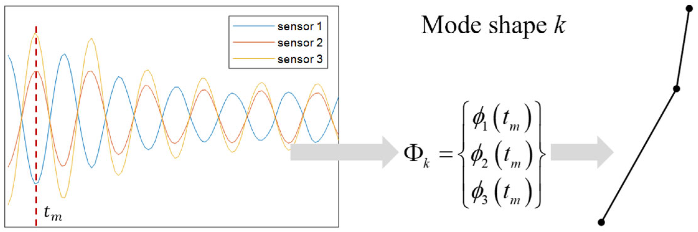
2.2. Identification of Mode Shapes
2.3. Response Surface-Based FE Model Updating Methodology
3. Field Modal Testing for PV Support Structure
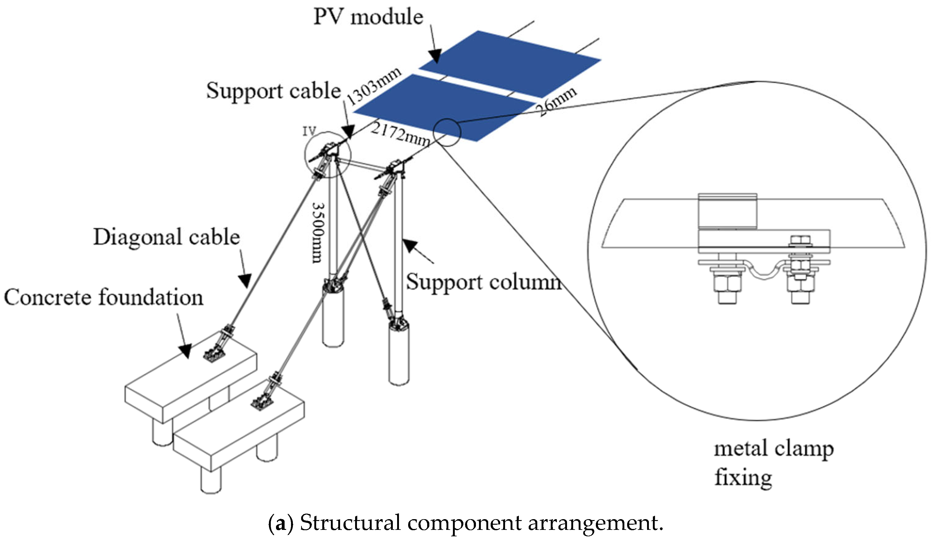
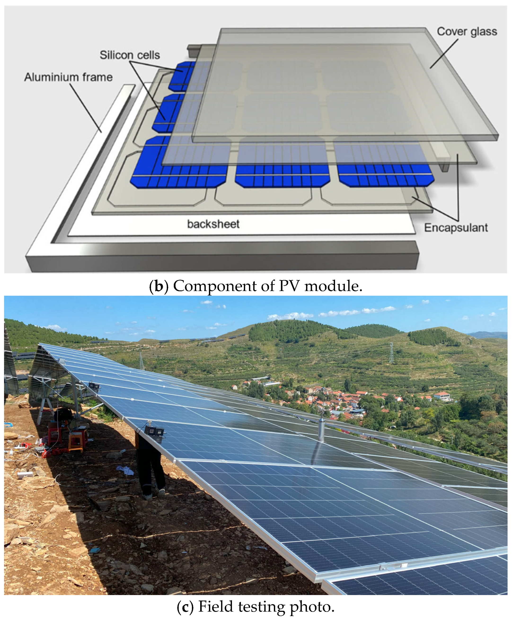
3.1. PV Support Structure
3.2. Field Modal Testing Scheme
3.3. Data from Field Modal Testing
4. Results and Analysis
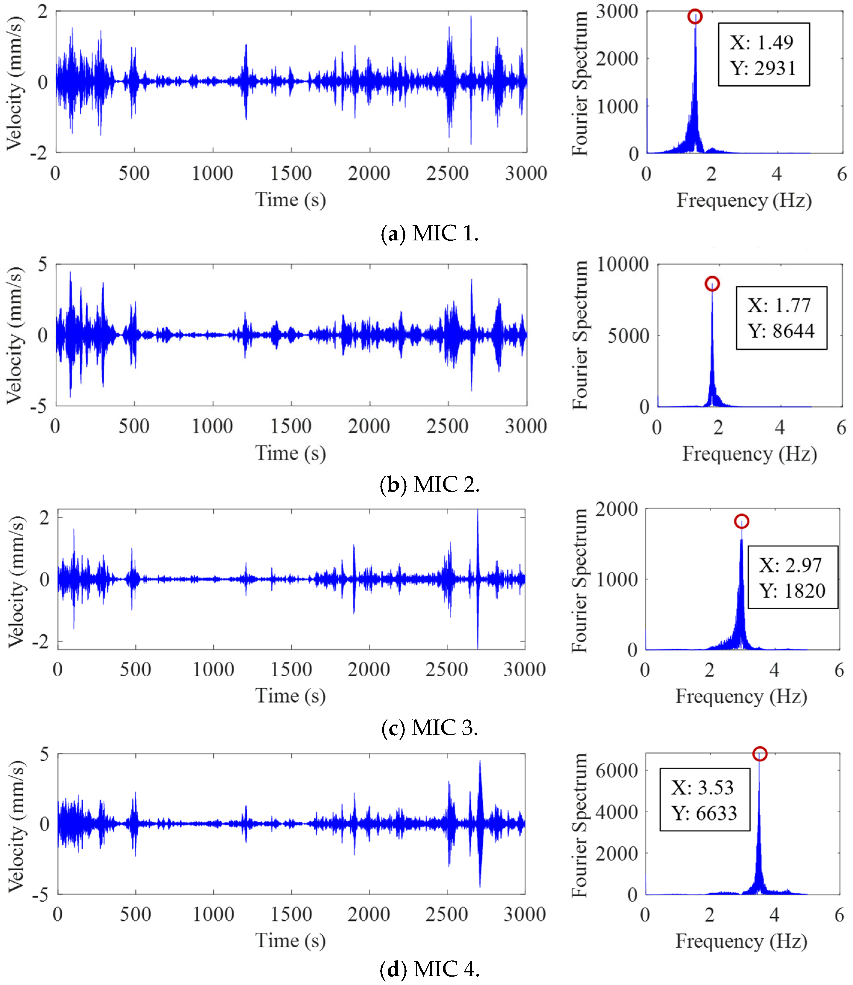
4.1. Modal Frequency and Damping Ratio Identification
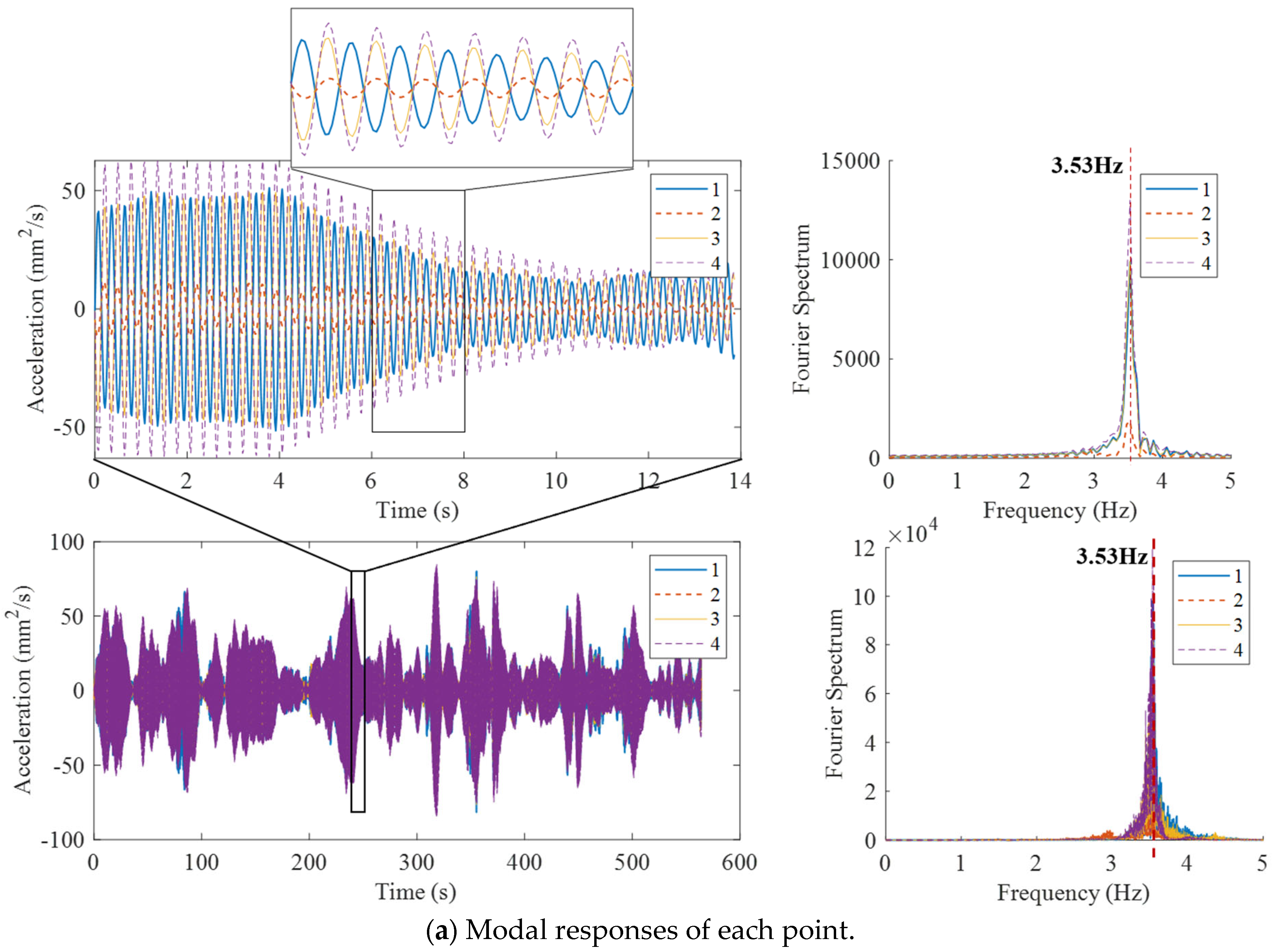
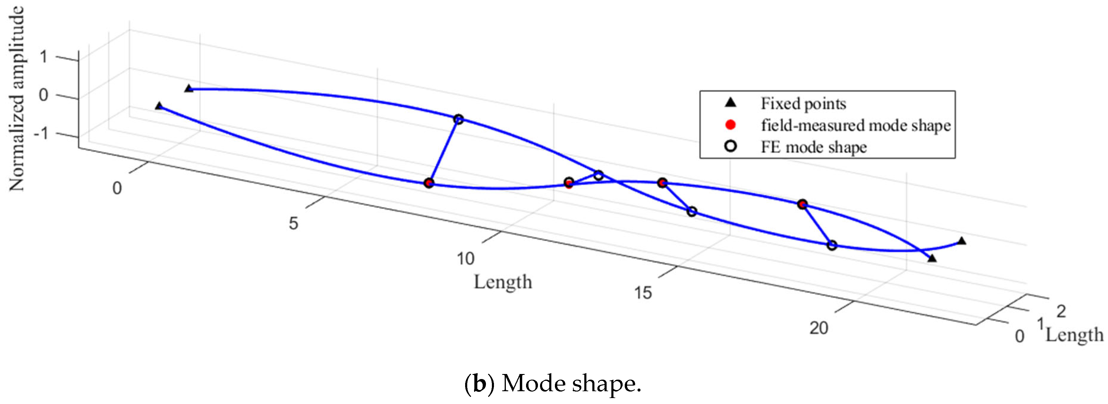
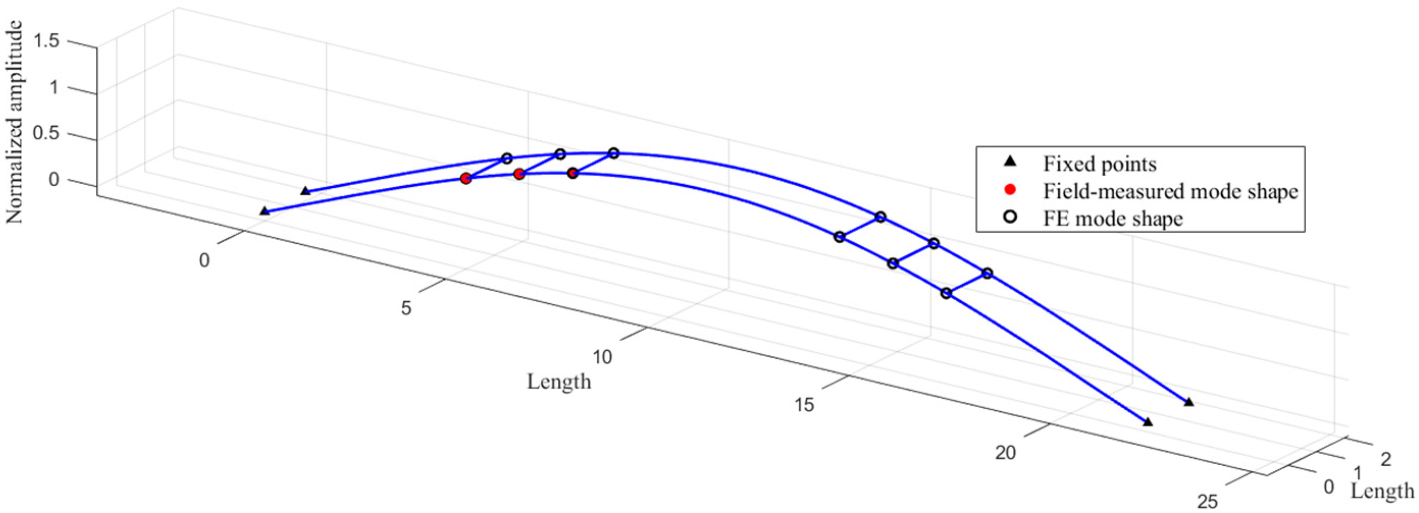
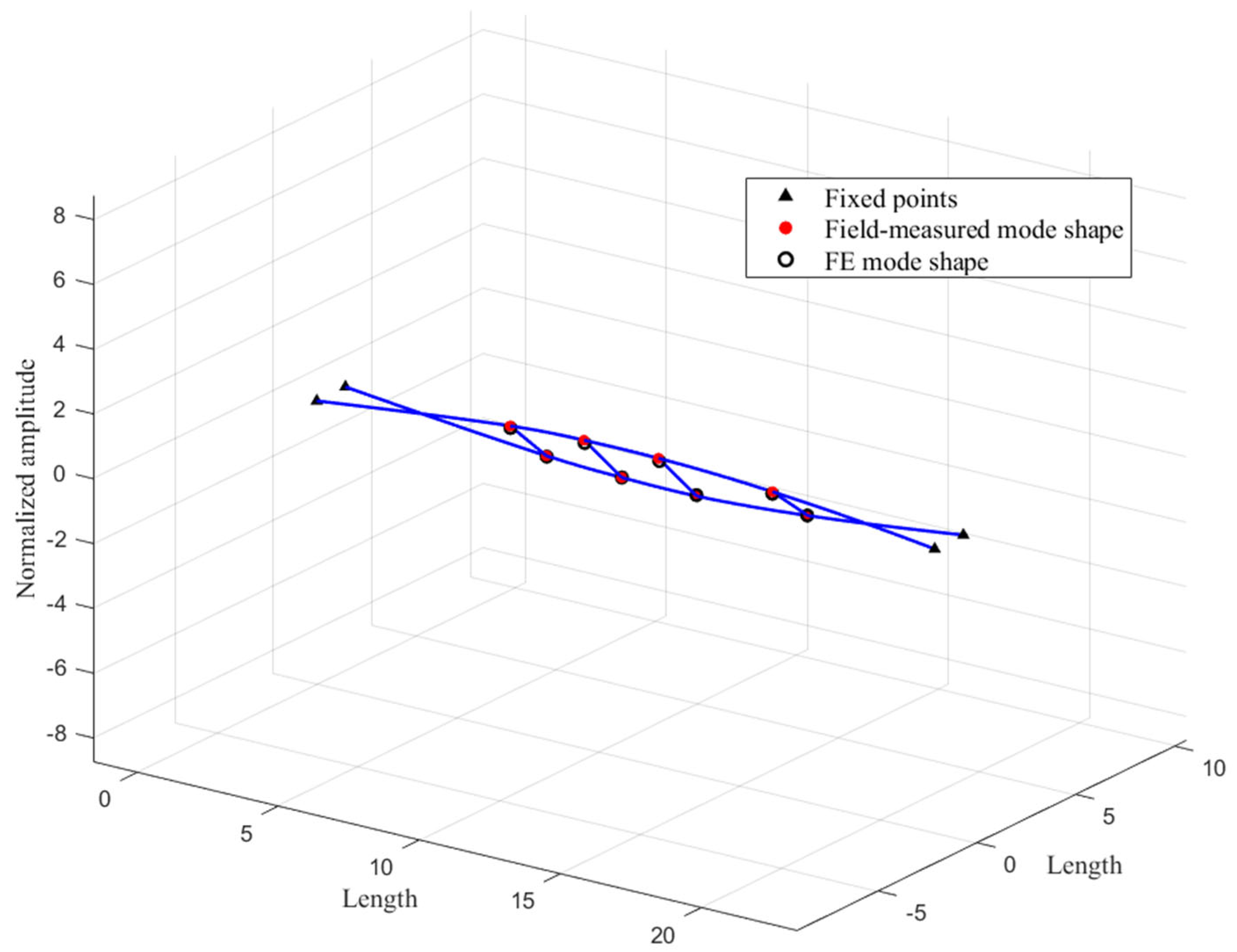
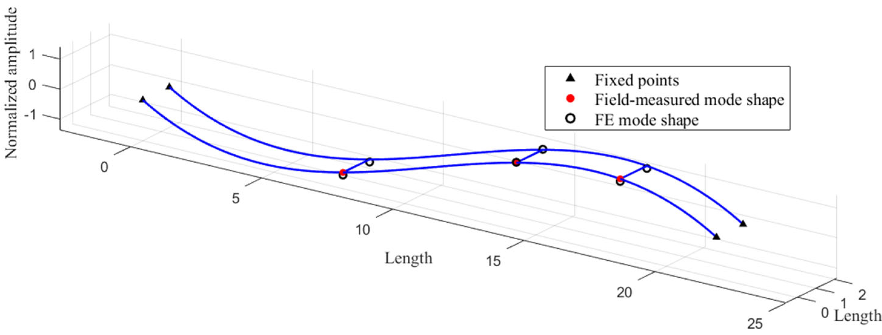
4.2. Mode Shape Identification
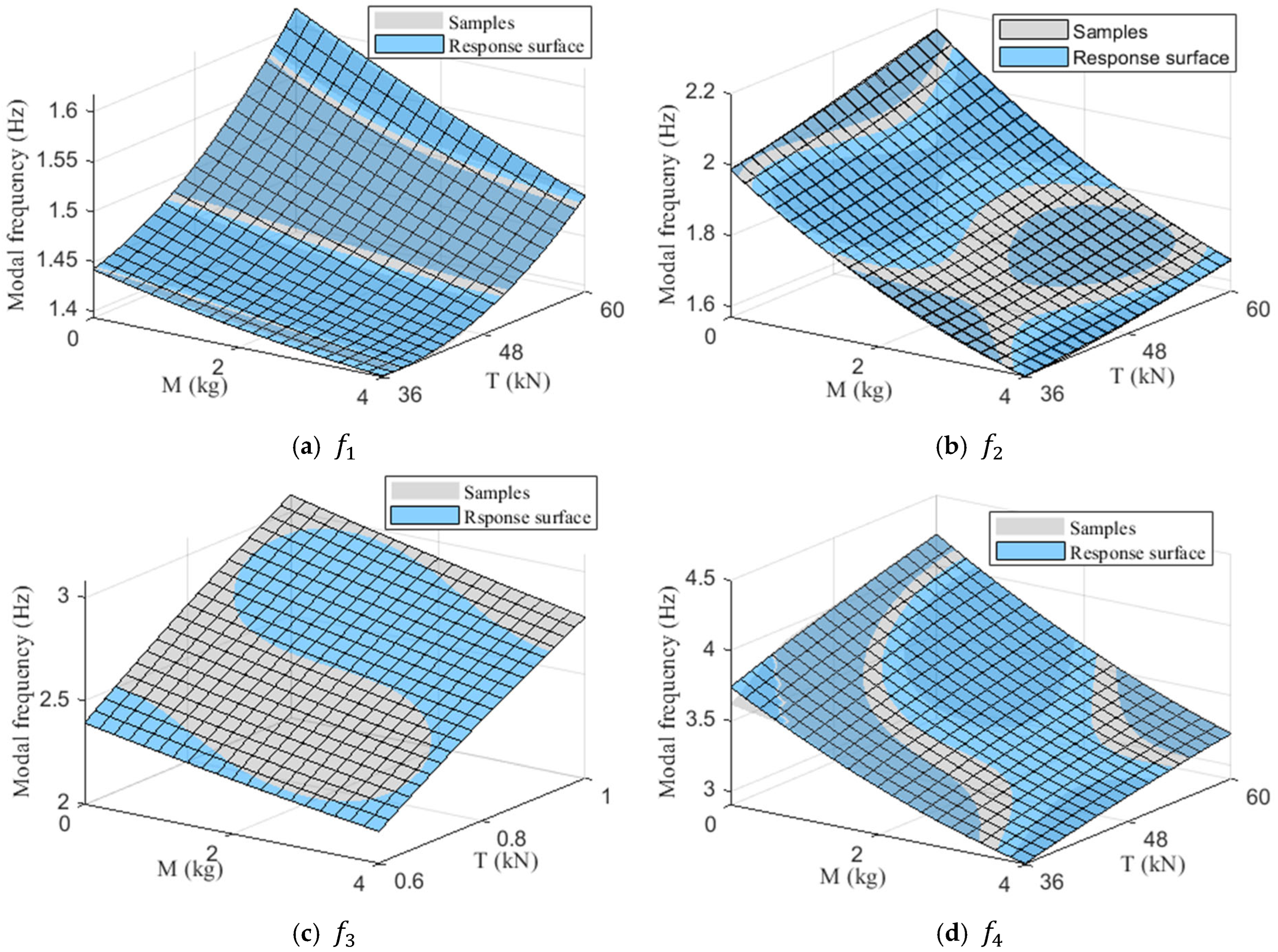
4.3. Response Surface Model
4.4. Finite Element Model Updating
5. Conclusions
- (1)
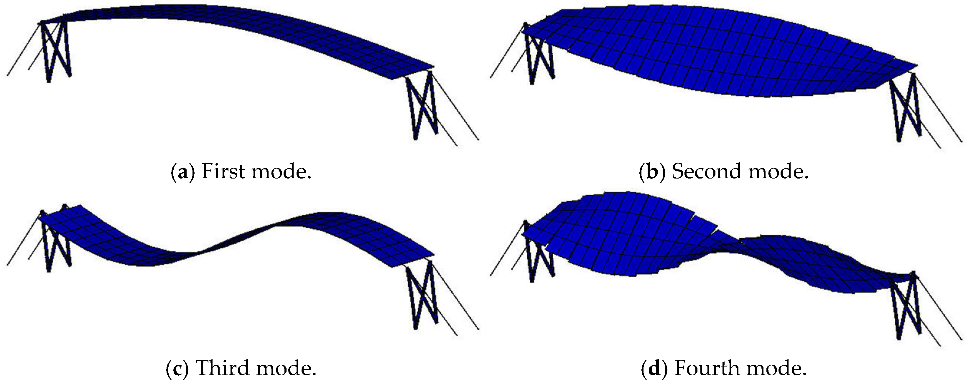
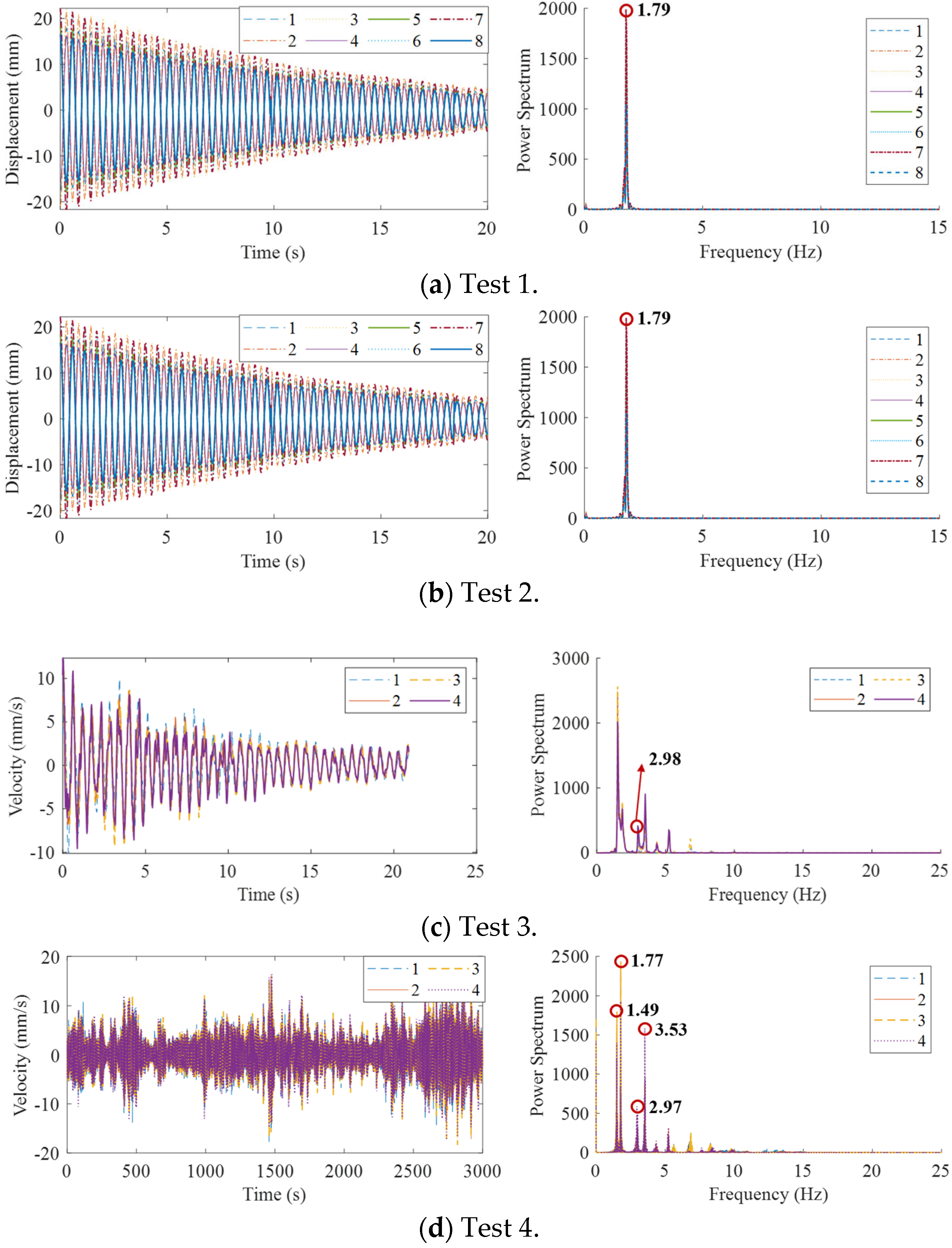
- The effectiveness of the field modal testing method was verified. The results indicate that computer vision-based measurement enables high-precision identification of the first two order vibration modes of the PV support structure. For high-order modes, due to weaker vibration energy, ambient excitation combined with velocity sensors are more suitable.
- (2)
- The first four modal properties of the flexible PV support structure were identified. The first four modal frequencies are 1.49 Hz, 1.79 Hz, 2.98 Hz, and 3.53 Hz, and the first four damping ratios are 1.7%, 0.7%, 1.3%, and 0.4%. It is noteworthy that the damping ratios of the first- and second-order torsional modes are only 0.7% and 0.4%, respectively, indicating that the low-damping characteristics of the flexible PV structure should be given particular attention in the design practice.
- (3)
- A response surface-based finite element model updating method for flexible PV support structures was proposed. Based on the FE model updating results, the modeling of flexible photovoltaic support structures should consider a cable tension reduction factor of 0.866, a 2 kg metal frame mass, and the modeling of the columns. Validation against field-measured modal frequencies demonstrates significant error reduction: relative discrepancies in the first four modes decreased from 13.61%, 23.92%, 3.36%, and 21.11% to 0.5%, 1.39%, 8.72%, and 0.54%. The high fitting accuracy of the response surface surrogate model demonstrates its feasibility as an alternative to full finite element analyses.
Author Contributions
Funding
Institutional Review Board Statement
Informed Consent Statement
Data Availability Statement
Acknowledgments
Conflicts of Interest
Abbreviations
| PV | Photovoltaic |
| FE | Finite element |
| PSO | Particle swarm optimization |
| VMD | Variational mode decomposition |
| NExT | Natural excitation technique |
| SDESA | Smoothed discrete energy separation algorithm |
| HCEO | Half-cycle energy operator |
| MIC | Mutually independent component |
References
- Ding, H.; He, X.; Jing, H.; Wu, X.; Weng, X. Design Method of Primary Structures of a Cost-Effective Cable-Supported Photovoltaic System. Appl. Sci. 2023, 13, 2968. [Google Scholar] [CrossRef]
- Dallaev, R.; Pisarenko, T.; Papež, N.; Holcman, V. Overview of the Current State of Flexible Solar Panels and Photovoltaic Materials. Materials 2023, 16, 5839. [Google Scholar] [CrossRef] [PubMed]
- Kim, S.; Quy, H.V.; Bark, C.W. Photovoltaic Technologies for Flexible Solar Cells: Beyond Silicon. Mater. Today Energy 2021, 19, 100583. [Google Scholar] [CrossRef]
- Zidane, T.E.K.; Aziz, A.S.; Zahraoui, Y.; Kotb, H.; AboRas, K.M.; Kitmo; Jember, Y.B. Grid-Connected Solar PV Power Plants Optimization: A Review. IEEE Access 2023, 11, 79588–79608. [Google Scholar] [CrossRef]
- Tamura, Y.; Kim, Y.C.; Yoshida, A.; Itoh, T. Wind-Induced Vibration Experiment on Solar Wing. MATEC Web Conf. 2015, 24, 04006. [Google Scholar] [CrossRef]
- Kim, Y.C.; Shan, W.; Yang, Q.S.; Tamura, Y.; Yoshida, A.; Ito, T. Effect of Panel Shapes on Wind-Induced Vibrations of Solar Wing System Under Various Wind Environments. J. Struct. Eng. 2020, 146, 04020104. [Google Scholar] [CrossRef]
- Kim, Y.; Tamura, Y.; Yoshida, A.; Ito, T.; Shan, W.; Yang, Q. Experimental Investigation of Aerodynamic Vibrations of Solar Wing System. Adv. Struct. Eng. 2018, 21, 2217–2226. [Google Scholar] [CrossRef]
- Liu, J.; Li, S.; Luo, J.; Chen, Z. Experimental Study on Critical Wind Velocity of a 33-Meter-Span Flexible Photovoltaic Support Structure and Its Mitigation. J. Wind. Eng. Ind. Aerodyn. 2023, 236, 105355. [Google Scholar] [CrossRef]
- Liu, J.; Li, S.; Chen, Z. Experimental Study on Effect Factors of Wind-Induced Response of Flexible Photovoltaic Support Structure. Ocean. Eng. 2024, 307, 118199. [Google Scholar] [CrossRef]
- Nan, B.; Chi, Y.; Jiang, Y.; Bai, Y. Wind Load and Wind-Induced Vibration of Photovoltaic Supports: A Review. Sustainability 2024, 16, 2551. [Google Scholar] [CrossRef]
- Ge, Y.; Wen, Z.; Fang, G.; Lou, W.; Xu, H.; Wang, G. Explicit Solution Framework and New Insights of 3-DOF Linear Flutter Considering Various Frequency Relationships. Eng. Struct. 2024, 307, 117883. [Google Scholar] [CrossRef]
- Ding, H.; He, X.; Jing, H.; Wu, X.; Weng, X. Shielding and Wind Direction Effects on Wind-Induced Response of Cable-Supported Photovoltaic Array. Eng. Struct. 2024, 309, 118064. [Google Scholar] [CrossRef]
- He, X.H.; Ding, H.; Jing, H.Q.; Zhang, F.; Wu, X.P.; Weng, X.J. Wind-Induced Vibration and Its Suppression of Photovoltaic Modules Supported by Suspension Cables. J. Wind. Eng. Ind. Aerodyn. 2020, 206, 104275. [Google Scholar] [CrossRef]
- Bao, T.; Li, Z.; Pu, O.; Chan, R.W.K.; Zhao, Z.; Pan, Y.; Yang, Y.; Huang, B.; Wu, H. Modal Analysis of Tracking Photovoltaic Support System. Sol. Energy 2023, 265, 112088. [Google Scholar] [CrossRef]
- Lei, Z.H. Research on Wind-Induced Vibration Characteristics and Control of Large-Span Cable-Supported Photovoltaic Support Brackets Structure by Experimental Test. Master’s Thesis, Central South University, Changsha, China, 2023. [Google Scholar]
- White, F.E. Data Fusion Lexicon, Joint Directors of Laboratories, Technical Panel for C3, Data Fusion Sub-Panel; Naval Ocean Systems Center: San Diego, CA, USA, 1987. [Google Scholar]
- Smyth, A.; Wu, M. Multi-Rate Kalman Filtering for the Data Fusion of Displacement and Acceleration Response Measurements in Dynamic System Monitoring. Mech. Syst. Signal Process. 2007, 21, 706–723. [Google Scholar] [CrossRef]
- Yang, M.; Wu, J.; Zhang, Q. GNSS and Accelerometer Data Fusion by Variational Bayesian Adaptive Multi-Rate Kalman Filtering for Dynamic Displacement Estimation of Super High-Rise Buildings. Eng. Struct. 2025, 325, 119396. [Google Scholar] [CrossRef]
- Moschas, F.; Stiros, S. Measurement of the Dynamic Displacements and of the Modal Frequencies of a Short-Span Pedestrian Bridge Using GPS and an Accelerometer. Eng. Struct. 2011, 33, 10–17. [Google Scholar] [CrossRef]
- Luo, L.; Liu, Z.; Liu, H. Operational Modal Analysis Method for Long-Span Suspension Bridges Based on Data Fusion. In Proceedings of the 2024 4th International Conference on Computer Science and Blockchain (CCSB), Shenzhen, China, 6–8 September 2024; IEEE: Piscataway, NJ, USA, 2024. [Google Scholar]
- Zhu, H.; Gao, K.; Xia, Y. Multi-rate data fusion for dynamic displacement measurement of beam-like supertall structures using acceleration and strain sensors. Struct. Health Monit. 2019, 19, 520–536. [Google Scholar] [CrossRef]
- Zhang, Q.; Fu, X.; Ren, L.; Li, H.-N. Two-Dimensional Full-Field Displacement Reconstruction of Lattice Towers Using Data Fusion Method: Theoretical Study and Experimental Validation. Thin-Walled Struct. 2023, 182, 110189. [Google Scholar] [CrossRef]
- Huang, M.; Li, X.; Cai, K.; Kareem, A. Motion Adaptive Vision-Based Vibration Measurement and Modal Identification for the Roof Masts of a Tall Building. Eng. Struct. 2025, 323, 119278. [Google Scholar] [CrossRef]
- Park, J.W.; Moon, D.S.; Yoon, H.; Gomez, F.; Spencer Jr, B.F.; Kim, J.R. Visual-Inertial Displacement Sensing Using Data Fusion of Vision-Based Displacement with Acceleration. Struct. Control. Health Monit. 2018, 25, e2122. [Google Scholar] [CrossRef]
- Ma, Z.; Choi, J.; Sohn, H. Real-Time Structural Displacement Estimation by Fusing Asynchronous Acceleration and Computer Vision Measurements. Comput.-Aided Civ. Infrastruct. Eng. 2022, 37, 688–703. [Google Scholar] [CrossRef]
- Xiu, C.; Weng, Y.; Shi, W. Vision and Vibration Data Fusion-Based Structural Dynamic Displacement Measurement with Test Validation. Sensors 2023, 23, 4547. [Google Scholar] [CrossRef] [PubMed]
- Xu, Z.; Hou, G.; Zhang, Z.; Wang, W.; Fan, H.; Shi, J. Numerical analysis of wind-induced vibration coefficient of fish-belt PV cable truss. Sol. Energy 2019, 2, 46–49. (In Chinese) [Google Scholar]
- Du, H.; Xu, H.W.; Zhang, Y.L. Wind pressure characteristics and wind vibration response of long-span flexible photovoltaic support structure. J. Harbin Inst. Technol. 2022, 54, 67–74. (In Chinese) [Google Scholar]
- Song, Y.M.; Yuan, H.X.; Du, X.X.; Wang, R.L. Research on static and dynamic response of single layer flexible photovoltaic support structure. Build. Struct. 2023, 1–8. (In Chinese) [Google Scholar]
- Wang, Z.G.; Zhao, F.F.; Ji, C.M.; Peng, X.F.; Shen, T. Analysis of vibration control of multi-row large-span flexible photovoltaic supports. Eng. J. Wuhan Univ. 2020, 53, 29–34. (In Chinese) [Google Scholar]
- Wang, Z.G.; Zhao, F.F.; Ji, C.M.; Peng, X.F.; Shen, T. Wind-induced vibration analysis of multi-row and multi-span flexible photovoltaic support. Eng. J. Wuhan Univ. 2021, 54, 75–79. (In Chinese) [Google Scholar]
- Wang, Z.G.; Zhao, F.F.; Ji, C.M.; Peng, X.F.; Shen, T. A comparative analysis of wind vibration response of large-span flexible photovoltaic support with stabilizing cable. Eng. J. Wuhan Univ. 2022, 55, 33–38. (In Chinese) [Google Scholar]
- Smith, S.W.; Beattie, C.A. Secant-method adjustment for structural models. AIAA J. 1991, 29, 119–126. [Google Scholar] [CrossRef]
- Levin, R.I.; Waters, T.P.; Lieven, N.A. Required precision and valid methodologies for dynamic finite element model updating. J. Vib. Acoust. 1998, 120, 733–741. [Google Scholar] [CrossRef]
- Friswell, M.I.; Mottershead, J.E. Finite Element Model Updating in Structural Dynamics; Springer: Berlin, Germany, 1995; Volume 3, pp. 45–78. [Google Scholar]
- Mottershead, J.E.; Friswell, M.I. Model updating in structural dynamics: A survey. J. Sound vibration 1993, 167, 347–375. [Google Scholar] [CrossRef]
- Link, M. Updating of analytical models—Review of numerical procedures and application aspects. In Structural Dynamics Forum SD2000; Research Studies Press Ltd.: Baldock, UK, 2001. [Google Scholar]
- Guo, Q.T.; Zhang, L.M. Finite element model updating based on response surface methodology. In Proceedings of the 22nd IMAC, Dearborn, MI, USA, 26–29 January 2004. [Google Scholar]
- Ren, W.X.; Fang, S.E.; Deng, M.Y. Response Surface–Based Finite-Element-Model Updating Using Structural Static Responses. J. Eng. Mech. 2011, 137, 248–257. [Google Scholar] [CrossRef]
- Fang, S.E. Studies on Structural Damage Detection by Finite Element Model Updating. Ph.D. Thesis, Central South University, Changsha, China, 2010. [Google Scholar]
- Cai, K.; Huang, M.; Li, X.; Xu, H.; Li, B.; Yang, C. Modal Parameter Identification of Tall Buildings Based on Variational Mode Decomposition and Energy Separation. Wind. Struct. 2023, 37, 445–460. [Google Scholar] [CrossRef]
- Dragomiretskiy, K.; Zosso, D. Variational Mode Decomposition. IEEE Trans. Signal Process. 2014, 62, 531–544. [Google Scholar] [CrossRef]
- James, G.H. The natural excitation technique (NExT) for modal parameter extraction from operating structures. J. Anal. Exp. Modal Anal. 1995, 10, 260. [Google Scholar]
- Maragos, P.; Kaiser, J.F.; Quatieri, T.F. Energy Separation in Signal Modulations with Application to Speech Analysis. IEEE Trans. Signal Process. 1993, 41, 3024–3051. [Google Scholar] [CrossRef]
- Huang, F.L.; Wang, X.M.; Chen, Z.Q.; He, X.H.; Ni, Y.Q. A New Approach to Identification of Structural Damping Ratios. J. Sound Vib. 2007, 303, 144–153. [Google Scholar] [CrossRef]
- Wang, D.; Tan, D.; Liu, L. Particle swarm optimization algorithm: An overview. Soft Comput. 2018, 22, 387–408. [Google Scholar] [CrossRef]
- Bagheri, A.; Ozbulut, O.E.; Harris, D.K. Structural System Identification Based on Variational Mode Decomposition. J. Sound Vib. 2018, 417, 182–197. [Google Scholar] [CrossRef]
- Allemang, R.J. The Modal Assurance Criterion—Twenty Years of Use and Abuse. Sound Vib. 2003, 37, 14–23. [Google Scholar]
- Xu, H.; Ding, K.; Shen, G.; Du, H.; Chen, Y. Experimental Investigation on Wind-Induced Vibration of Photovoltaic Modules Supported by Suspension Cables. Eng. Struct. 2024, 299, 117125. [Google Scholar] [CrossRef]
- Li, J.W.; He, Y.J.; Quan, Y. Study on wind vibration coefficient of single-layer cable-suspended photovoltaic support. J. Archit. Civ. Eng. 2024, 41, 63–70. (In Chinese) [Google Scholar] [CrossRef]
- Yang, Z.; He, Y.J.; Quan, Y. Static analysis and simplified calculation method of single-layer cable-suspended photovoltaic support. Sci. Technol. Eng. 2022, 22, 9252–9259. (In Chinese) [Google Scholar]


| Instruments | Model | Technical Parameters |
|---|---|---|
| CMOS camera (Baumer VCXU-53C, Frauenfeld, Switzerland) |  | Camera chip: PYTHON5000 Maximum resolution: 2592 × 2048 Pixel size: 4.8 μm Chroma: RGB |
| Lens (Computar V3528-MPY, Mebane, NC, USA) |  | Focal length: 35 mm Relative aperture: F = 1:2.8 Variable aperture range: 2.8~16 TV distortion: −0.1% |
| Velocity Sensor (EY521V) |  | Sensitivity: 5.71 m/s resolution: 4 × 10⁻⁷ m/s frequency range: 0.5~100 Hz Maximum speed: 0.3 m/s |
| Test Cases | Target Mode | Excitation Method | Sensor Type | Placement Method | Test Duration |
|---|---|---|---|---|---|
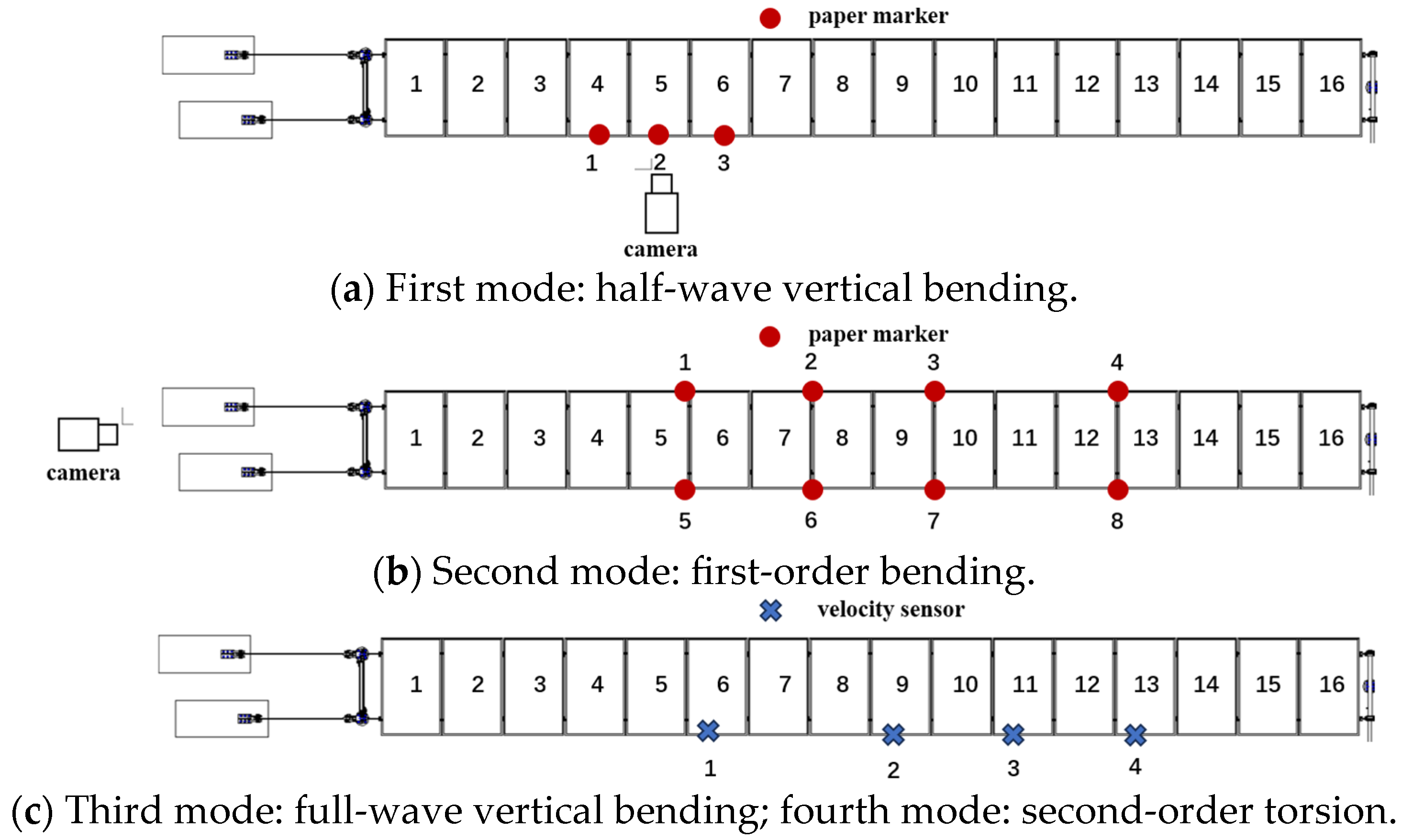
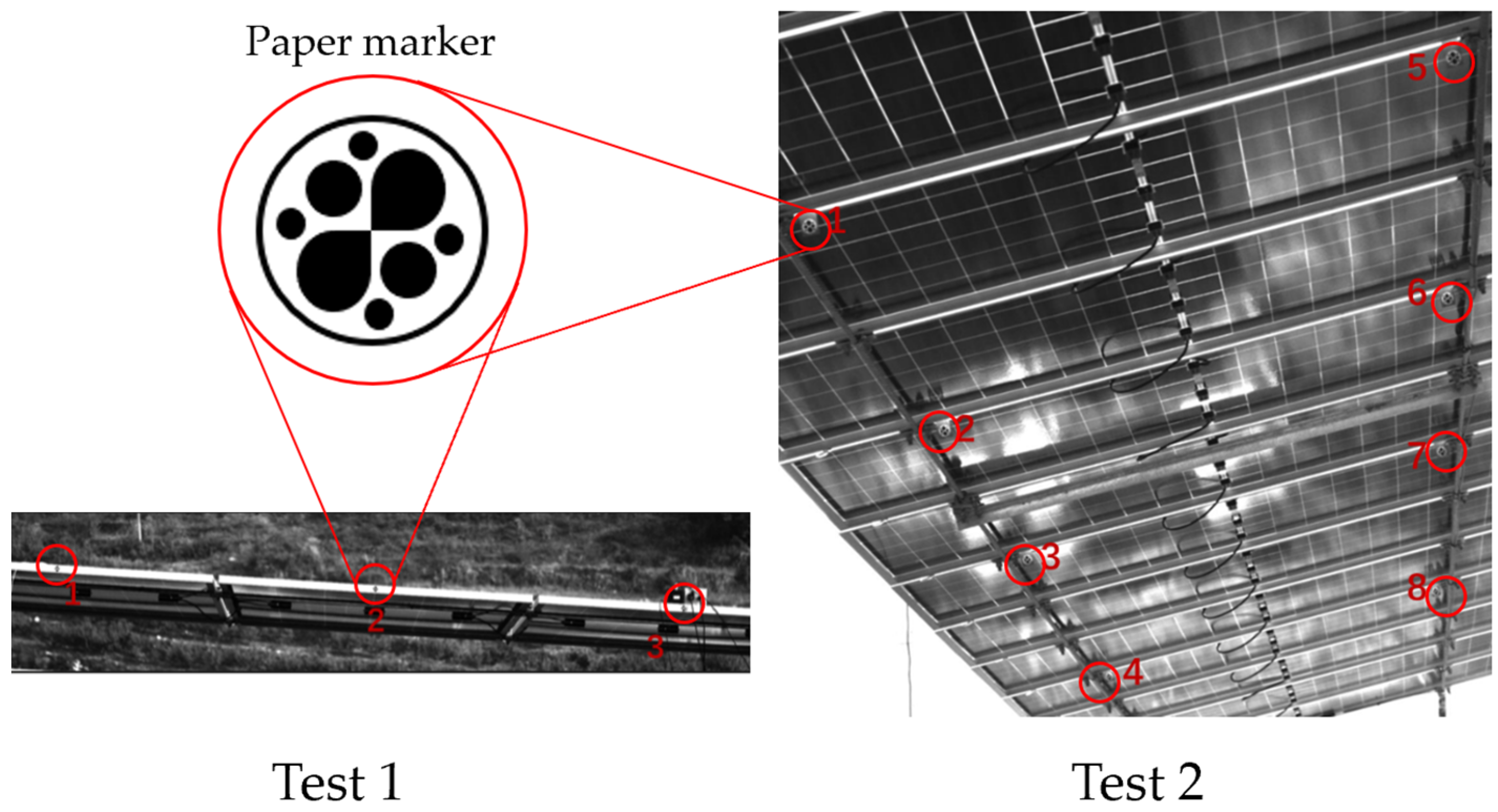
| 1 | half-wave vertical bending | 1/2 span, vertical harmonic loads | Vison-based measurement | Figure 8a | 5 min |
| 2 | first-order torsion | 1/2 span, vertical synchronized opposite-direction harmonic loads | Vison-based measurement | Figure 8b | 5 min |
| 3 | full-wave vertical bending | 1/4 and 3/4 span, vertical synchronized opposite-direction harmonic loads | Velocity sensor | Figure 8c | 5 min |
| 4 | second-order torsion | Ambient excitation | Velocity sensor | Figure 8c | 120 min |
| Mode | by SH | by HT | |
|---|---|---|---|
| 1 | 1.488 | 0.0172 | 0.0155 |
| 2 | 1.775 | 0.0065 | 0.0071 |
| 3 | 2.980 | 0.0098 | 0.013 |
| 4 | 3.526 | 0.0035 | 0.0043 |
| Mode | Method | Mode Shape Vector | 1-MAC | |||||||
|---|---|---|---|---|---|---|---|---|---|---|
| 1 | 2 | 3 | 4 | 5 | 6 | 7 | 8 | |||
| 1 | Field- measured | 0.73 | 0.88 | 1 | / | / | / | / | / | 3.33 × 10⁻⁶ |
| FEM | 0.72 | 0.88 | 1 | / | / | / | / | / | ||
| 2 | Field- measured | 0.88 | 1 | 0.99 | 0.74 | −0.88 | −1 | −0.99 | −0.74 | 8.38 × 10⁻⁵ |
| FEM | 0.86 | 1 | 1 | 0.73 | −0.86 | −0.1 | −0.99 | −0.73 | ||
| 3 | Field- measured | 0.69 | / | −0.75 | 1 | / | / | / | / | 5.18 × 10⁻² |
| FEM | 0.82 | / | −0.82 | 1 | / | / | / | / | ||
| 4 | Field- measured | 0.83 | 0.15 | −0.79 | 1 | / | / | / | / | 3.41 × 10⁻² |
| FEM | 0.79 | 0.18 | −0.79 | 1 | / | / | / | / | ||
| Response Features | Modal Frequencies (Hz) | Relative Error (%) | |
|---|---|---|---|
| FE | Field-Measured | ||
| f1 | 1.693 | 1.488 | 13.78 |
| f2 | 2.205 | 1.775 | 24.22 |
| f3 | 3.081 | 2.980 | 3.38 |
| f4 | 4.242 | 3.526 | 20.31 |
| Updating Parameters | Initial Value | Lower Bound | Upper Bound |
|---|---|---|---|
| (kN) | 60 | 36 | 60 |
| (kg) | 0 | 0 | 4 |
| 0 | 0 | 1 |
| Index | f1 | f2 | f3 | f4 |
|---|---|---|---|---|
| R2 | 0.998 | 1.000 | 1.000 | 0.998 |
| RMSE | 2.10 × 10⁻³ | 2.00 × 10⁻³ | 5.79 × 10⁻⁴ | 1.230 × 10⁻² |
| Updating Parameter | Initial | Optimization |
|---|---|---|
| (kg) | 0 | 2.00 |
| (kN) | 60 | 51.96 |
| Response Feature | Field-Measured | Initial Value | Updated Value | Initial Error | Updated Error |
|---|---|---|---|---|---|
| f1 (Hz) | 1.488 | 1.693 | 1.481 | 13.78% | 0.47% |
| f2 (Hz) | 1.775 | 2.205 | 1.802 | 24.22% | 1.52% |
| f3 (Hz) | 2.980 | 3.081 | 2.728 | 3.38% | 8.46% |
| f4 (Hz) | 3.526 | 4.242 | 3.516 | 20.31% | 0.28% |
Disclaimer/Publisher’s Note: The statements, opinions and data contained in all publications are solely those of the individual author(s) and contributor(s) and not of MDPI and/or the editor(s). MDPI and/or the editor(s) disclaim responsibility for any injury to people or property resulting from any ideas, methods, instructions or products referred to in the content. |
© 2025 by the authors. Licensee MDPI, Basel, Switzerland. This article is an open access article distributed under the terms and conditions of the Creative Commons Attribution (CC BY) license (https://creativecommons.org/licenses/by/4.0/).
Share and Cite
Huang, M.; Yang, C.; Cai, K.; Li, X. Modal Identification and Finite Element Model Updating of Flexible Photovoltaic Support Structures Using Multi-Sensor Data. Appl. Sci. 2025, 15, 5919. https://doi.org/10.3390/app15115919
Huang M, Yang C, Cai K, Li X. Modal Identification and Finite Element Model Updating of Flexible Photovoltaic Support Structures Using Multi-Sensor Data. Applied Sciences. 2025; 15(11):5919. https://doi.org/10.3390/app15115919
Chicago/Turabian StyleHuang, Mingfeng, Chen Yang, Kang Cai, and Xianzhe Li. 2025. "Modal Identification and Finite Element Model Updating of Flexible Photovoltaic Support Structures Using Multi-Sensor Data" Applied Sciences 15, no. 11: 5919. https://doi.org/10.3390/app15115919
APA StyleHuang, M., Yang, C., Cai, K., & Li, X. (2025). Modal Identification and Finite Element Model Updating of Flexible Photovoltaic Support Structures Using Multi-Sensor Data. Applied Sciences, 15(11), 5919. https://doi.org/10.3390/app15115919