Investigation of the Stress Intensity Factor in Heterogeneous Materials Based on the Postprocessing Routine of Commercial Finite Element Software

Abstract

An improved interaction integral method has been proposed for heterogeneous materials with complex interfaces based on the postprocessing routine of commercial finite element software. This approach introduces a suitably designed auxiliary field to eliminate the derivative terms of material parameters in the interaction integral, which enables the direct extraction of the stress intensity factor at the crack tip without considering the material interfaces. This paper utilizes the postprocessing routine of commercial finite element software to extract the simulation results from the specified analysis step to obtain the stress intensity factor. Validation via homogeneous material cases shows excellent agreement with the theoretical solutions. For two-dimensional/three-dimensional heterogeneous materials, the domain-independence of the present method still stands, even when the integral domain intersects interfaces. This new method improves the efficiency of parameter extraction and extends the scope of application of commercial finite element software for calculating the fracture parameters of heterogeneous materials.

1. Introduction

Composite materials are now widely used in many fields, such as aircraft fuselages and spacecraft propellant tanks, due to their ability to withstand harsh conditions. At present, numerous composite materials and structures with heterogeneous properties have been successfully developed and manufactured. Composite materials usually contain complex interfaces, which serve as nucleation sites for cracks, voids, and other defects. Therefore, in comparison to homogeneous materials, composite materials are more susceptible to fracture and failure [1].

A crucial aspect of analyzing crack propagation issues is the effective determination of crack-tip parameters. Crack tip fracture mechanics’ characteristic parameters mainly include stress intensity factors (SIFs), strain energy release rate (G), and crack tip opening displacement (COD). Among them, the stress intensity factor, the most widely used fracture mechanics parameter [2], is of great value in characterizing the stress, strain, and displacement fields near the crack tip. Methods for solving stress intensity factors can be divided into direct and indirect methods. Direct methods include displacement and stress methods, which calculate results via interpolation formulas but suffer from limited accuracy. In contrast, the J-integral method, a path-independent contour integral method, has the advantage of obtaining integral values independent of path selection, making it especially suitable for solving stress intensity factors at crack tips in heterogeneous materials.

Taking the crack problem of two-dimensional linear elastic materials as an example, its J-integral can be defined as follows:

$$J=\underset{\mathrm{\Gamma }\to 0}{\lim }{\displaystyle {\int }_{\mathrm{\Gamma }}(W{\delta }_{1i}-{\sigma }_{ij}{u}_{j,1})n_{i}d\mathrm{\Gamma }},$$

(1)

In this equation, W represents the strain energy density.

$$W={\displaystyle \frac{1}{2}}{\sigma }_{ij}{\epsilon }_{ij}={\displaystyle \frac{1}{2}}{C}_{ijkl}{\epsilon }_{ij}{\epsilon }_{kl}={\displaystyle \frac{1}{2}}{S}_{ijkl}{\sigma }_{ij}{\sigma }_{kl},$$

(2)

In this equation, ${\delta }_{ij}$ is the Kronecker delta, $C_{ijkl}$ and $S_{ijkl}$ are the stiffness and compliance tensors, respectively, and $n_i$ is the unit outward normal vector to the integration path $\mathrm{\Gamma }$, as shown in Figure 1.

Nevertheless, it is difficult to separate Mode I and Mode II stress intensity factors in mixed-mode fracture problems using the J-integral method. In the development of the J-integral method, the interaction integral method has shown significant advantages in calculating the mixed-mode stress intensity factors. By superimposing the actual and auxiliary fields, the mixed-mode stress intensity factors can be efficiently separated [3]. After years of theoretical refinement and algorithmic optimization by researchers, this method has proven to provide a advantage for the fracture analysis of linear elastic materials with complex interfaces [4,5]. Figure 2 illustrates a simulation of crack propagation in complex interfacial materials using the interaction integral method. Wang et al. [6] used the interaction integral method to calculate the stress intensity factors of mixed-mode cracks in anisotropic homogeneous materials. Subsequently, Nakamura [7] established a three-dimensional integral solution method for the stress intensity factors of bimaterial interface cracks, enabling the precise extraction of crack tip fracture parameters through a suitable auxiliary field. Tabaza et al. [8] proposed an unstructured tetrahedral element interaction integral method, addressing the path independence issue in three-dimensional functionally graded material crack analysis. Nahta and Moran [9] successfully applied the interaction integral method to axisymmetric interface crack analysis, while Gosz et al. [10] applied it to three-dimensional interface cracks with curved crack fronts. Gosz and Moran [11] further proposed an interaction integral method for solving stress intensity factors along three-dimensional curved crack fronts and calculated the stress intensity factors for spherical crack surfaces. Nagashima et al. [12] and Sukumar et al. [13] developed an extended finite element-based interaction integral method to output the stress intensity factors for interface cracks. Cisilino and Ortiz [14,15] used the interaction integral method to analyze two-dimensional and three-dimensional cracks within a boundary element framework. Merzbacher and Horst [16] applied this method to solve the stress intensity factors for internal cracks in laminated orthotropic materials. Scholars like Kim and Paulino [17], Yildirim [18], Duflot [19], and Pathak [20] have conducted in-depth studies on the interaction integral method, promoting its widespread application in fracture mechanics research on linear elastic materials, functionally graded materials, piezoelectric materials, and magnetoelectric materials. Zhu et al. [21] proposed an extended domain-independent interaction integral method for dynamic fracture problems under impact loading. This method addresses the influence of inertial effects and material rate-dependent properties on the crack tip field. In recent years, Guo et al. [22] and Yu et al. [23] have conducted extensive work on the interaction integral for complexly interfaced in heterogeneous linear elastic materials, proposing an interaction integral model with domain-independence and establishing a fracture mechanics analysis method for linear elastic materials with complex interfaces under mechanical and thermal loads. Yu and Kuna [24] summarized and reviewed the development of the interaction integral method over the past 20 years, highlighting its advantages and future trends in solving crack tip fracture mechanics parameters.

Current research on the interaction integral method primarily focuses on its engineering applications and algorithmic optimizations. However, the pre-processing steps, such as model construction and mesh generation, often rely on custom programming implementations, rendering the computational workflow cumbersome and time-consuming. Because of this, this paper improved an interaction integral method for heterogeneous materials with complex interfaces based on the postprocessing routine of ABAQUS. The present integral interaction method is deeply embedded in the finite element simulation platform, which enables the efficient and precise extraction of crack-tip fracture parameters in heterogeneous materials with complex interfaces.

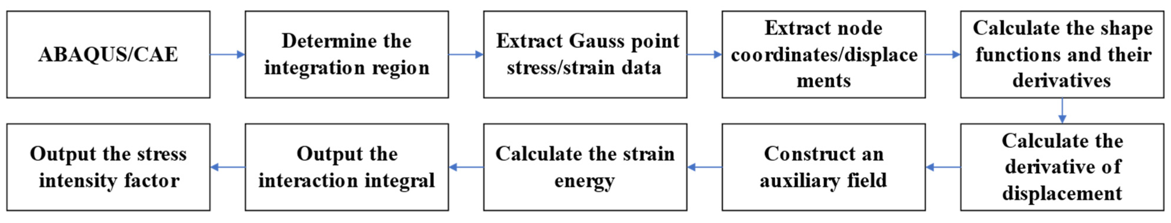
2. Fracture Parameter Solution Method Based on the Postprocessing Routine of ABAQUS

Finite element methods, such as ABAQUS, ANSYS, etc., have shown powerful pre-processing capabilities in model creation and mesh generation. This paper integrates the finite element method, ABAQUS 2022, with the interaction integral method to solve the crack problems in heterogeneous materials. By adopting a postprocessing routine, a Python v.3.11 program was written to extract the physical fields obtained from ABAQUS and substitute them into theoretical formulas. This approach allows for the rapid calculation of the interaction integral for complex models. The complete calculation procedure is illustrated in Figure 3. The following sections provide a detailed description of each step.

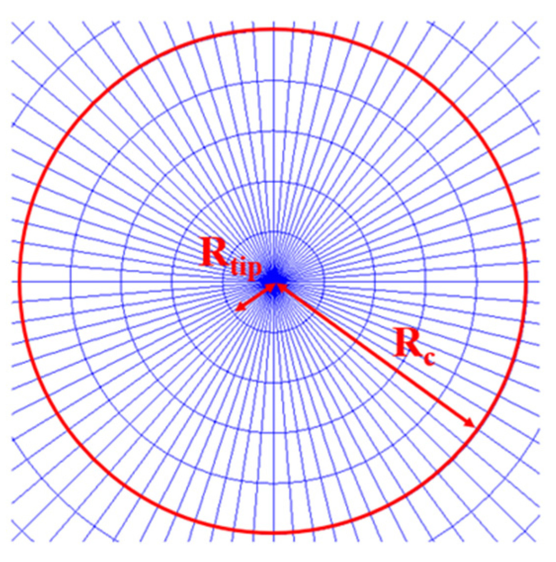
2.1. Selection of Integration Domain and Extraction of ABAQUS Result

After completing finite element modeling, crack setup, and meshing in ABAQUS, the result files are obtained through numerical computation. To ensure the accuracy of the subsequent fracture mechanics parameter calculations, the selection of an appropriate integration region is crucial. In this study, we define integration regions using circular paths with varying radii centered at the crack tip. The integration domains are established by creating these paths and tallying the finite elements they encompass or intersect. Additionally, the stress and strain fields at Gaussian integration points and the nodal displacement fields from ABAQUS results are extracted for the interaction integral computation. For the Jacobian matrix computation in the later finite element analysis, the global coordinates of nodes within the integration region are selected. Figure 4 illustrates the nodal and integration point locations for a four-node isoparametric linear element in a two-dimensional plane problem.

2.2. Construction of Auxiliary Fields

The interaction integral is the interaction part of the J-integral under actual and auxiliary fields. Choosing a proper auxiliary field can improve the efficiency of the derivation of the interaction integral. This section elaborates on the mathematical definition of the auxiliary field and develops a relevant calculation program.

Table 1. List of symbols.

Symbol	Meaning	Unit/Definition
E	Young’s modulus	MPa
$\nu$	Poisson’s ratio	/
u	Actual displacement	/
σ	Actual stress	/
ε	Actual strain	/
r	Radial coordinate	mm
θ	Angular coordinate	°
uaux	Auxiliary displacement	/
σaux	Auxiliary stress	/
εaux	Auxiliary strain	/
W	Strain energy density	J/mm3
C	Stiffness matrix	/
S	Compliance matrix	/
Stip	Compliance matrix at crack tip	/
J	J-integral	J/mm2
I	Interaction integral	J/mm2
K	Stress intensity factor	MPa·m1/2
q	Weight function	/
μ	Shear modulus	MPa
KI	Mode I stress intensity factor	MPa·m1/2
KII	Mode II stress intensity factor	MPa·m1/2
KIII	Mode III stress intensity factor	MPa·m1/2

lists the meanings of symbols in the formulas of the article.

For isotropic heterogeneous materials, the auxiliary field is typically defined in three ways: (1) equilibrium equation residuals; (2) compatibility equation residuals; (3) constant constitutive tensor equation. In this study, the second form is chosen, where the low-order terms of Williams’ crack-tip field for an infinite plate are used as the auxiliary field [25]. The auxiliary strain is derived from the actual material properties and the auxiliary stress field. The specific form is as follows:

$$u_i^{\mathrm{aux}}=K_{\mathrm{I}}^{\mathrm{aux}}\sqrt{{\displaystyle \frac{r}{2\mathsf{\pi }}}}{f}_i^{\mathrm{I}}(\theta ,S^{\mathrm{tip}})+K_{\mathrm{II}}^{\mathrm{aux}}\sqrt{{\displaystyle \frac{r}{2\mathsf{\pi }}}}{f}_i^{\mathrm{II}}(\theta ,S^{\mathrm{tip}}),$$

(3)

$${\sigma }_{ij}^{\mathrm{aux}}={\displaystyle \frac{K_{\mathrm{I}}^{\mathrm{aux}}}{\sqrt{2\mathsf{\pi }r}}}{g}_{ij}^{\mathrm{I}}(\theta ,S^{tip})+{\displaystyle \frac{K_{\mathrm{II}}^{\mathrm{aux}}}{\sqrt{2\mathsf{\pi }r}}}{g}_{ij}^{\mathrm{II}}(\theta ,S^{tip}),$$

(4)

$$\begin{array}{cc}{\epsilon }_{ij}^{\mathrm{aux}}=S_{ijkl}(x){\sigma }_{kl}^{\mathrm{aux}},& (i,j,k,l=1,2),\end{array}$$

(5)

In these equations, r and $\theta$ are polar coordinates. $S_{\mathrm{tip}}$ and $S_{ijkl}$ represent the compliance tensor and its components, respectively. For isotropic materials, the functions $f_i^{\mathrm{I}}$,$f_i^{\mathrm{II}}$, $g_i^{\mathrm{I}}$ and $g_i^{\mathrm{II}}$ are as follows:

$$\begin{array}{cc}{f}_1^{\mathrm{I}}={\displaystyle \frac{1}{2{\mu }_{\mathrm{tip}}}}\cos {\displaystyle \frac{\theta }{2}}\left({\kappa }_{\mathrm{tip}}-1+2{\sin }^2{\displaystyle \frac{\theta }{2}}\right),& f_1^{\mathrm{II}}={\displaystyle \frac{1}{2{\mu }_{\mathrm{tip}}}}\sin {\displaystyle \frac{\theta }{2}}\left({\kappa }_{\mathrm{tip}}+1+2{\cos }^2{\displaystyle \frac{\theta }{2}}\right),\\ f_2^{\mathrm{I}}={\displaystyle \frac{1}{2{\mu }_{\mathrm{tip}}}}\sin {\displaystyle \frac{\theta }{2}}\left({\kappa }_{\mathrm{tip}}+1-2{\cos }^2{\displaystyle \frac{\theta }{2}}\right),& f_2^{\mathrm{II}}=-{\displaystyle \frac{1}{2{\mu }_{\mathrm{tip}}}}\cos {\displaystyle \frac{\theta }{2}}\left({\kappa }_{\mathrm{tip}}-1-2{\sin }^2{\displaystyle \frac{\theta }{2}}\right)\end{array},$$

(6)

$$\begin{array}{l}\begin{array}{cc}{g}_{11}^{\mathrm{I}}=\cos {\displaystyle \frac{\theta }{2}}\left(1-\sin {\displaystyle \frac{\theta }{2}}\sin {\displaystyle \frac{3\theta }{2}}\right),& g_{11}^{\mathrm{II}}=-\sin {\displaystyle \frac{\theta }{2}}\left(2+\cos {\displaystyle \frac{\theta }{2}}\cos {\displaystyle \frac{3\theta }{2}}\right)\end{array}\\ \begin{array}{cc}{g}_{22}^{\mathrm{I}}=\cos {\displaystyle \frac{\theta }{2}}\left(1+\sin {\displaystyle \frac{\theta }{2}}\sin {\displaystyle \frac{3\theta }{2}}\right),& g_{22}^{\mathrm{II}}=\sin {\displaystyle \frac{\theta }{2}}\cos {\displaystyle \frac{\theta }{2}}\cos {\displaystyle \frac{3\theta }{2}}\end{array}\\ \begin{array}{cc}{g}_{12}^{\mathrm{I}}=g_{21}^{\mathrm{I}}=g_{22}^{\mathrm{II}},& g_{12}^{\mathrm{II}}=g_{21}^{\mathrm{II}}=g_{11}^{\mathrm{I}}\end{array}\end{array},$$

(7)

and

$${\kappa }_{\mathrm{tip}}=\left\{\begin{array}{cc}{\displaystyle \frac{3-{\nu }_{\mathrm{tip}}}{1+{\nu }_{\mathrm{tip}}}}& (\mathrm{Plane} \mathrm{stress})\\ 3-4{\nu }_{\mathrm{tip}}& (\mathrm{Plane} \mathrm{strain})\end{array}\right.,$$

(8)

In the equation, ${\mu }_{\mathrm{tip}}$ and ${\nu }_{\mathrm{tip}}$ are the shear modulus and Poisson’s ratio of the material at the crack tip.

2.3. Computation of Interaction Integral

The interaction integral (abbreviated as I-integral), also known as the interaction energy integral or the M-integral, is a two-state integral derived from the J-integral of the actual and specified auxiliary fields. Due to the designability of the auxiliary field in the I-integral, it has been widely used for various homogeneous, heterogeneous, and composite materials to determine critical fracture parameters such as stress intensity factors (SIFs) and T-stresses [26].

For linear elastic materials, stress, strain, and displacement satisfy the principle of superposition. Calculate the J-integral under the combined actual and auxiliary fields using Equation (1) to obtain the following:

$$J^S=\underset{\mathrm{\Gamma }\to 0}{\lim }{\displaystyle {\int }_{\mathrm{\Gamma }}[\frac{1}{2}({\sigma }_{ij}+{\sigma }_{ij}^{\mathrm{aux}})({\epsilon }_{ij}+{\epsilon }_{ij}^{\mathrm{aux}}){\delta }_{1i}-({\sigma }_{ij}+{\sigma }_{ij}^{\mathrm{aux}})(u_{j,1}+u_{j,1}^{\mathrm{aux}})]n_{i}d\mathrm{\Gamma }}=J+J^{\mathrm{aux}}+I,$$

(9)

After rearrangement, the equation can be divided into three parts: the J-integral for the actual field alone, the J-integral for the auxiliary field alone, and the interaction term between the actual and auxiliary fields. The interaction term is as follows:

$$I=\underset{\mathrm{\Gamma }\to 0}{\lim }{\displaystyle {\int }_{\mathrm{\Gamma }}[\frac{1}{2}({\sigma }_{jk}{\epsilon }_{jk}^{\mathrm{aux}}+{\sigma }_{jk}^{\mathrm{aux}}{\epsilon }_{jk}){\delta }_{1i}-({\sigma }_{ij}{u}_{j,1}^{\mathrm{aux}}+{\sigma }_{ij}^{\mathrm{aux}}{u}_{j,1})]n_{i}d\mathrm{\Gamma }}$$

(10)

Equation (10) is defined as the interaction integral. $\mathrm{\Gamma }$ is an infinitesimal closed loop including the crack tip.

As the interaction integral defined above is a line integral around an infinitesimal crack tip contour, it cannot be directly solved in finite element calculations. Therefore, we need to convert it into an area integral. There are two primary methods to accomplish this. The first method transforms the line integral in Equation (10) into the difference between a finite contour integral and an area integral of the surrounding region. The second method involves multiplying the integral in Equation (10) by a weighting function to directly convert it into an equivalent area integral. The first method may result in larger computational errors when calculating the line integral [27]. Therefore, this study adopts the second method to convert the line integral into an area integral. The weight function q is defined as 1 within the integration radius and 0 outside. According to Reference [23], the converted equivalent area integral form is as follows:

$$I={\displaystyle {\int }_A({\sigma }_{ij}{u}_{j,1}^{\mathrm{aux}}+{\sigma }_{ij}^{\mathrm{aux}}{u}_{j,1}-{\sigma }_{jk}^{\mathrm{aux}}{\epsilon }_{jk}{\delta }_{1i})q_{,i}dA}+{\displaystyle {\int }_A(-f_j{u}_{j,1}^{\mathrm{aux}}+{\sigma }_{ij}{u}_{j,i1}^{\mathrm{aux}}-{\sigma }_{ij,1}^{\mathrm{aux}}{\epsilon }_{ij})qdA},$$

(11)

In the equation, A is an area of finite size, including the crack tip, and $f_j$ is the body force of the element. Based on the crack tip strain field, equilibrium equations without body forces $f_j=0$, and the constitutive equations, Equation (11) can be expressed as follows:

$$I={\displaystyle {\int }_A({\sigma }_{ij}{u}_{j,1}^{\mathrm{aux}}+{\sigma }_{ij}^{\mathrm{aux}}{u}_{j,1}-{\sigma }_{jk}^{\mathrm{aux}}{\epsilon }_{jk}{\delta }_{1i})q_{,i}dA}+{\displaystyle {\int }_A{\sigma }_{ij}[S_{ijkl}^{\mathrm{tip}}-S_{ijkl}(x)]{\sigma }_{kl,1}^{\mathrm{aux}}qdA}$$

(12)

For heterogeneous materials, the elements within the integration region and the crack tip may be located in different materials, so there are different material parameters. The calculation of Equation (12) requires only the material properties at the crack tip and integration points, without involving the derivatives of material parameters. Thus, this form of interaction integral does not require differentiable material parameters, and compared to the traditional form, it broadens the applicable scope.

To enhance its computational efficiency, Equation (12) is transformed into the Gaussian quadrature summation form of Equation (13). A program is then written to iterate over all Gaussian points within the integration domain, perform weighted accumulation, and ultimately output the interaction integral terms.

$$I={{\displaystyle \sum _{e=1}^{e_A}{\displaystyle \sum _{p=1}^{p_e}\left\{\left({\sigma }_{ij}^{\mathrm{aux}}{u}_{j,1}^{AB}+{\sigma }_{ij}^{AB}{u}_{j,1}^{\mathrm{aux}}-{\sigma }_{jk}^{\mathrm{aux}}{\epsilon }_{jk}^{AB}{\delta }_{1i}\right)q_{,i}+{\sigma }_{ij}^{AB}[S_{ijkl}^{\mathrm{tip}}-S_{ijkl}(x)]{\sigma }_{kl,1}^{\mathrm{aux}}q\right\}}}}_p{\left|J\right|}_p{w}_p$$

(13)

In the formula, $e_A$ denotes the number of elements within integration area A, and $p_e$ represents the number of integration points within each element. ${\left|J\right|}_p$ is the determinant of the Jacobian matrix, $w_p$ is the weight coefficient for integration point p, and $u_{j,1}^{AB}$, ${\sigma }_{ij}^{AB}$, ${\epsilon }_{ij}^{AB}$ are the derivatives of displacement, strain tensor, and stress tensor component data obtained via the post-processing of the ABAQUS finite element computation results.

For three-dimensional cases, the interaction integral form for calculating stress intensity factors is similar to that in two-dimensional problems. The equivalent volume integral form of the interaction integral for a three-dimensional crack front is as follows:

$$\overline{I}={\displaystyle {\int }_V(u_{i,l}{\sigma }_{ij}^{\mathrm{aux}}}{q}_{l,j}+u_{i,l}^{\mathrm{aux}}{\sigma }_{ij}{q}_{l,j}-{\sigma }_{ij}^{\mathrm{aux}}{\epsilon }_{ij}{q}_{l,l})dV+{\displaystyle {\int }_V(u_{i,l}{\sigma }_{ij,j}^{\mathrm{aux}}+u_{i,lj}^{\mathrm{aux}}{\sigma }_{ij}-u_{i,l}^{\mathrm{aux}}{f}_i-{\sigma }_{ij,l}^{\mathrm{aux}}{\epsilon }_{ij})q_{l}dV},$$

(14)

The interaction integral at point s on the crack front can be expressed as follows:

$$I(s)={\displaystyle \frac{\overline{I}}{{\displaystyle {\int }_{L_c}△}a(p)dl}},$$

(15)

In the equation, $\Delta a(p)$ represents the virtual extension length of the crack front.

2.4. Computation of Stress Intensity Factors

After obtaining the interaction integral results, it is necessary to decompose and extract various types of stress intensity factors to determine the mixed-mode crack conditions. This is based on the relationship between the J-integral, strain energy release rate, and stress intensity factors in isotropic materials, as follows:

$$J=G={\displaystyle \frac{1}{{E^{\prime }}_{\mathrm{tip}}}}(K_{\mathrm{I}}^2+K_{\mathrm{II}}^2),$$

(16)

and

$${E^{\prime }}_{\mathrm{tip}}=\left\{\begin{array}{cc}{E}_{\mathrm{tip}}& (\mathrm{Plane} \mathrm{stress})\\ {\displaystyle \frac{E_{\mathrm{tip}}}{1-v_{\mathrm{tip}}^2}}& (\mathrm{Plane} \mathrm{strain})\end{array}\right.,$$

(17)

$E_{tip}$ and ${\nu }_{tip}$ are the Young’s modulus and Poisson’s ratio at the crack tip, respectively. The J-integral under the combined actual and auxiliary fields is expressed as follows:

$$J^S={\displaystyle \frac{1}{E_{\mathrm{tip}}^{\prime }}}[{(K_{\mathrm{I}}+K_{\mathrm{I}}^{\mathrm{aux}})}^2+{(K_{\mathrm{II}}+K_{\mathrm{II}}^{\mathrm{aux}})}^2]=J+J^{\mathrm{aux}}+I,$$

(18)

The J-integral due to the auxiliary field alone is expressed as follows:

$$J^{\mathrm{aux}}={\displaystyle \frac{1}{E_{\mathrm{tip}}^{\prime }}}[{(K_{\mathrm{I}}^{\mathrm{aux}})}^2+{(K_{\mathrm{II}}^{\mathrm{aux}})}^2],$$

(19)

The interaction integral is expressed as follows:

$$I={\displaystyle \frac{2}{E_{\mathrm{tip}}^{\prime }}}(K_{\mathrm{I}}{K}_{\mathrm{I}}^{\mathrm{aux}}+K_{\mathrm{II}}{K}_{\mathrm{II}}^{\mathrm{aux}}),$$

(20)

Substituting $\begin{array}{cc}{K}_{\mathrm{I}}^{\mathrm{aux}}=1,& K_{\mathrm{II}}^{\mathrm{aux}}=0\end{array}$ and $\begin{array}{cc}{K}_{\mathrm{I}}^{\mathrm{aux}}=0,& K_{\mathrm{II}}^{\mathrm{aux}}=1\end{array}$ into Equation (20), the Mode I and Mode II stress intensity factors are calculated via two interaction integral computations.

$$\begin{array}{cc}{K}_{\mathrm{I}}={\displaystyle \frac{E_{\mathrm{tip}}^{\prime }}{2}}{I}_{(1)},& K_{\mathrm{II}}={\displaystyle \frac{E_{\mathrm{tip}}^{\prime }}{2}}{I}_{(2)}\end{array},$$

(21)

where $I_{(1)}$ and $I_{(2)}$ denote the interaction integral values obtained from the two calculations.

For three-dimensional problems, the interaction integral and stress intensity factors satisfy the following relationship:

$$I(s)={\displaystyle \frac{2}{E^{\prime }(s)}}(K_{\mathrm{I}}{K}_{\mathrm{I}}^{\mathrm{aux}}+K_{\mathrm{II}}{K}_{\mathrm{II}}^{\mathrm{aux}})+{\displaystyle \frac{1}{\mu (s)}}{K}_{\mathrm{III}}{K}_{\mathrm{III}}^{\mathrm{aux}},$$

(22)

and

$$E^{\prime }(s)=\left\{\begin{array}{ll}E(s)& (\mathrm{Plane} \mathrm{stress})\\ {\displaystyle \frac{E(s)}{[1-{\nu }^2(s)]}}& (\mathrm{Plane} \mathrm{strain})\end{array}\right.,$$

(23)

$$\mu (s)={\displaystyle \frac{E(s)}{[2+2\nu (s)]}},$$

(24)

Set $K_{\mathrm{I}}^{\mathrm{aux}}=1,K_{\mathrm{II}}^{\mathrm{aux}}=K_{\mathrm{III}}^{\mathrm{aux}}=0$ in Equation (22) to obtain the Mode I stress intensity factor at point s. Similarly, adjust the coefficients to derive the Mode II and Mode III stress intensity factors.

2.5. The Advantages of the Present Method

The conventional J-integral can be expressed as follows:

$$J={\displaystyle {\int }_A({\sigma }_{ij}{u}_{j,1}-W{\delta }_{1i})q_{,i}dA}+{\displaystyle \frac{1}{2}}{\displaystyle {\int }_A{\sigma }_{ij}{S}_{ijkl,1}{\sigma }_{kl}qdA},$$

(25)

In the conventional J-integral, given by Equation (25), the derivatives of the material parameters are involved. Thus, the material properties must be differentiable when using the J-integral to solve the fracture parameters. However, in the interaction integral given by Equation (12), there are no derivative terms of material parameters. This means it does not require differentiable material properties. Instead, it only needs to calculate the difference between the material parameters at the integration point and the crack tip.

For complex material interface cases, the interaction integral can be expressed as follows:

$$I={\displaystyle {\int }_A({\sigma }_{ij}{u}_{j,1}^{\mathrm{aux}}+{\sigma }_{ij}^{\mathrm{aux}}{u}_{j,1}-{\sigma }_{jk}^{\mathrm{aux}}{\epsilon }_{jk}{\delta }_{1i})q_{,i}dA}+{\displaystyle {\int }_A{\sigma }_{ij}[S_{ijkl}^{\mathrm{tip}}-S_{ijkl}(x)]{\sigma }_{kl,1}^{\mathrm{aux}}qdA}+I_{\mathrm{interface}}^{\ast },$$

(26)

After solving the interfacial integral $I_{\mathrm{interface}}^{\ast }$ in a curve coordinate system based on the material interface, it was found that $I_{\mathrm{interface}}^{\ast }=0$, meaning the material interface makes no contribution to the interaction integral. Therefore, the interaction integral form derived from Equation (12) also applies to the cases with material interfaces. Compared with the J-integral, the method proposed in this paper can solve the crack problems in heterogeneous materials whose material properties are discontinuous.

The present integral interaction method is deeply embedded in the finite element simulation platform using the postprocessing routine of ABAQUS. This makes the traditional finite element method capable of dealing with the fracture problems in heterogeneous materials with complex material interfaces.

3. Numerical Examples

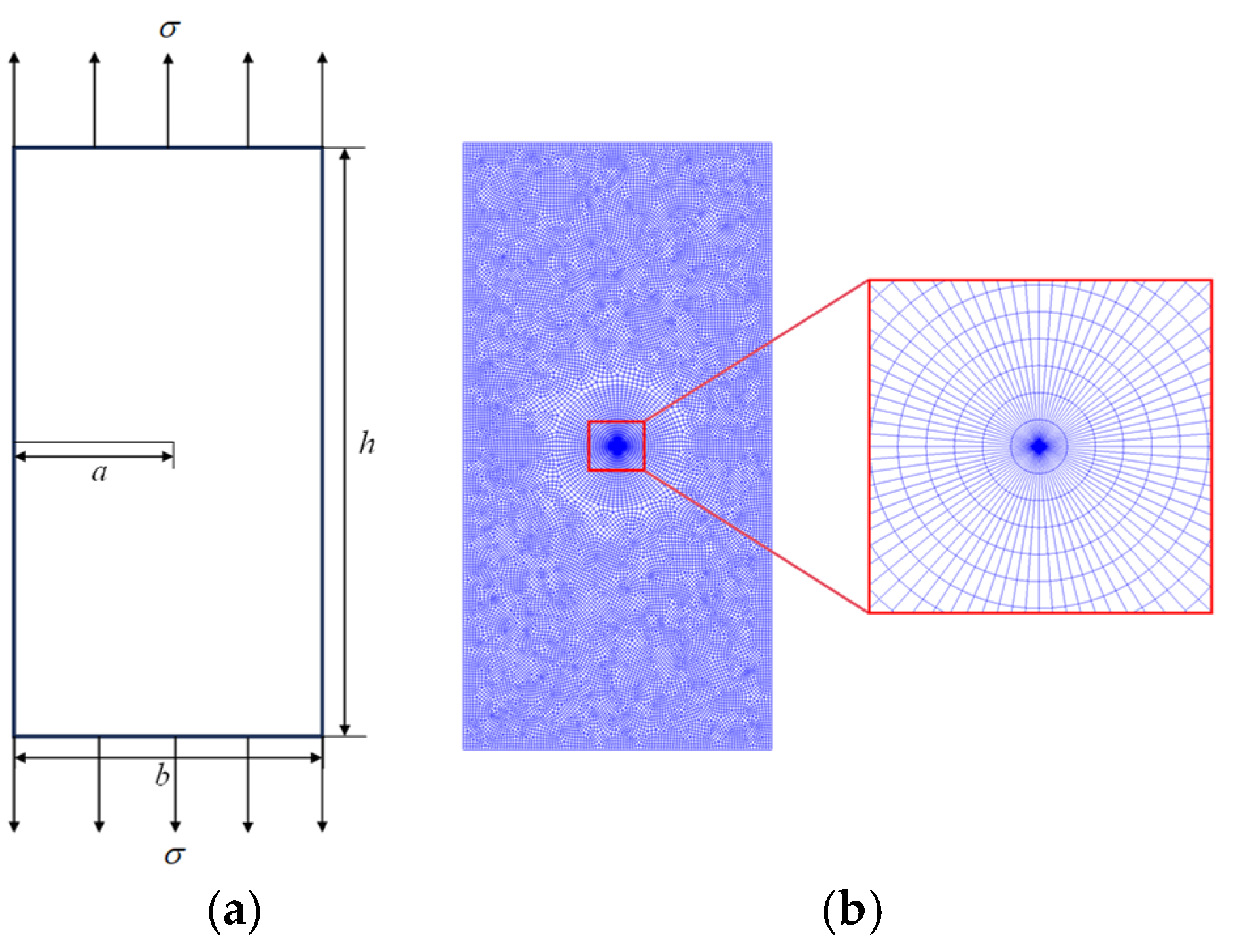
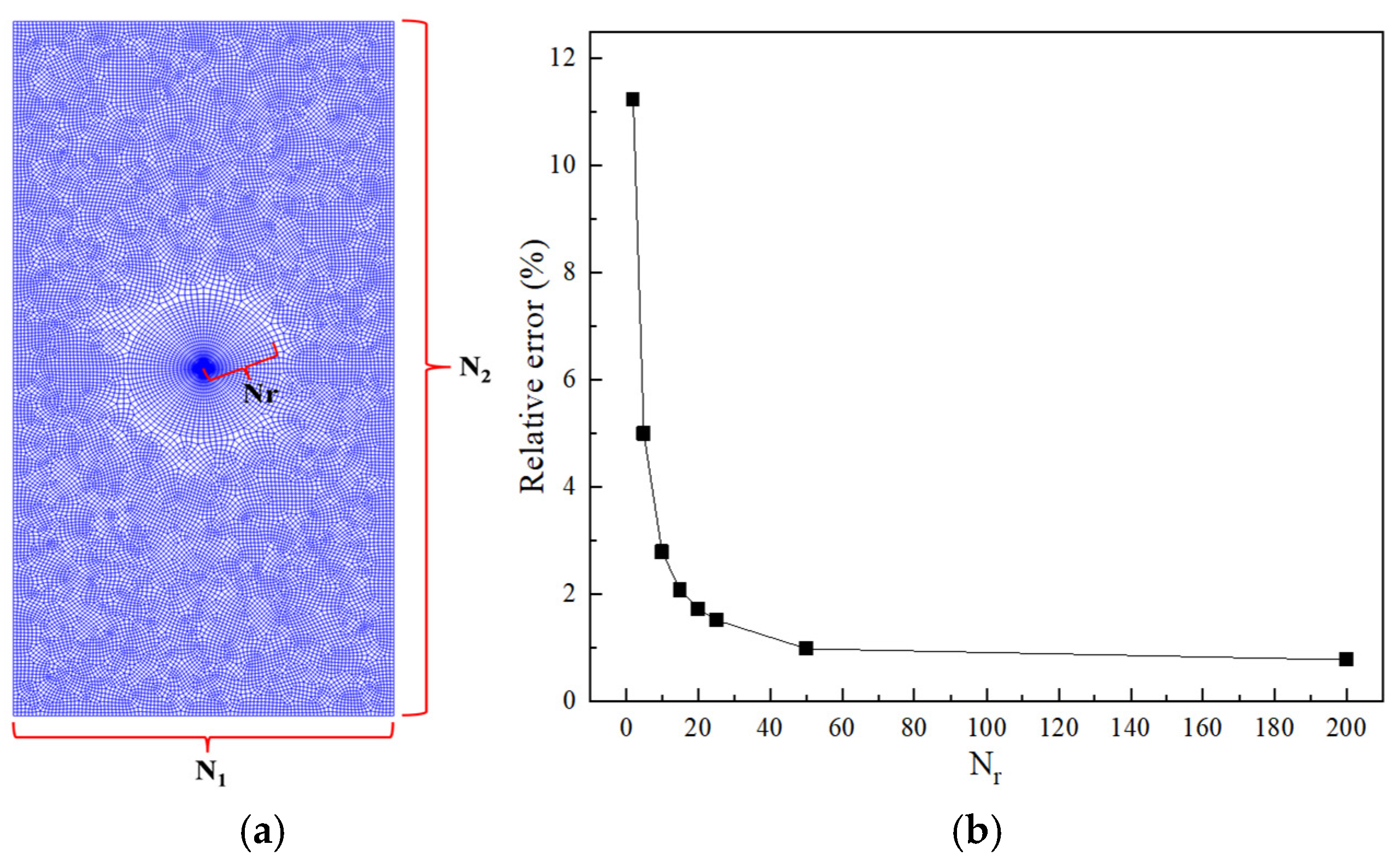
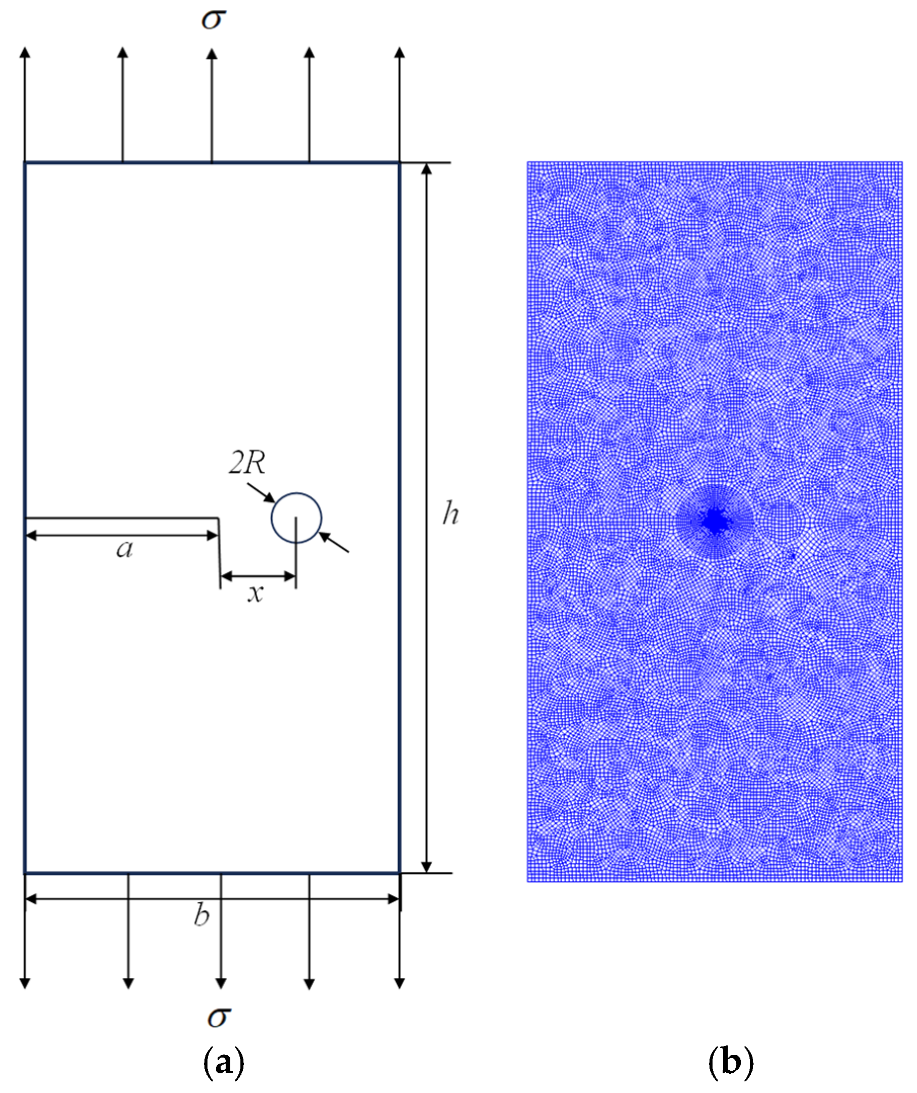
3.1. Numerical Examples of Homogeneous Material

To verify the accuracy of the method proposed in this paper, some typical numerical examples are selected.

(a)

Homogeneous Rectangular Plate with Edge Crack under Unidirectional Tensile Load

As shown in Figure 5a, a rectangular plate with length h = 100 mm and width b = 50 mm contains a horizontal edge crack of length a. The rectangular plate is subjected to uniform uniaxial tensile loads $\sigma =10 \mathrm{MPa}$ on upper and lower sides, with an elastic modulus and Poisson’s ratio of $E={10}^5 \mathrm{MPa}$ and $\nu =0.2$, respectively. The crack tip was implemented and defined using XFEM tools.

As shown in Figure 5b, the finite element mesh of the rectangular plate is presented for a/b = 0.5. Considering the singularity at the crack tip, CPS3 elements are utilized in the crack tip region to improve computational accuracy, while CPS4 elements are used in other areas. The entire mesh consists of 48,325 quadrilateral elements, 126 triangular elements, 48,451 elements in total and 48,919 nodes. The integral domain is selected as the region enclosed by a circle, with the crack tip as the center and a radius of 10 mm. The normalized factor is selected as $K_0=\sigma \sqrt{\pi a}$.

According to the crack state and load distribution of the model mentioned above, it is a mode I fracture problem. The theoretical solution of the mode I stress intensity factor is as follows:

$$K_{\mathrm{I}}=F\sigma \sqrt{\pi a},$$

(27)

$$F=1.12-0.23{\displaystyle \frac{a}{b}}+10.6{\left({\displaystyle \frac{a}{b}}\right)}^2-21.7{\left({\displaystyle \frac{a}{b}}\right)}^3+30.4{\left({\displaystyle \frac{a}{b}}\right)}^4,$$

(28)

Table 2. Normalized stress intensity factor of a homogeneous rectangular plate with an edge crack under a unidirectional tensile load.

a/b	Present	Theoretical	ABAQUS	Error A 1 [%]	Error B 2 [%]
0.1	1.176	1.184	1.171	0.7	0.4
0.2	1.362	1.373	1.360	0.8	0.1
0.3	1.653	1.665	1.651	0.7	0.1
0.4	2.098	2.113	2.101	0.7	0.1
0.5	2.821	2.843	2.823	0.8	0.1

¹ Error between the program and theoretical values. ² Error between the program and ABAQUS.

presents the normalized stress intensity factors from the present method, ABAQUS, and theoretical calculations at varying crack lengths (a/b). The results from the present method closely match those from ABAQUS and the theoretical solution, with relative errors below 0.8%. This provides evidence of the accuracy of the method.

(b)

Homogeneous Rectangular Plate with a Center-Inclined Crack Under Unidirectional Tensile Load

As shown in Figure 6a, there is a rectangular plate made of homogeneous material with a length of h = 62.5 mm and width of b = 50 mm. It has a central crack of length a = 25 mm, inclined at an angle β to the horizontal. The plate is subjected to uniform uniaxial tensile loads $\sigma =10 \mathrm{MPa}$ on the upper and lower sides, with a modulus of elasticity $E={10}^5 \mathrm{MPa}$ and Poisson’s ratio $\nu =0.2$.

As shown in Figure 6b, taking β = 45° as an example, the finite element meshes of the rectangular plate are presented. The CPS3 element is used at the crack tip with appropriate refinement to enhance the computational accuracy, and the CPS4 element is used for other parts. The entire mesh consists of 10,953 quadrilateral elements, 210 triangular elements, a total of 11,163 elements, and 11,280 nodes. The integral domain is the area enclosed by a circle with a radius of 10 mm centered at the crack tip. The normalized factor was selected as $K_0=\sigma \sqrt{\pi a}$.

Table 3. Normalized stress intensity factor of a homogeneous rectangular plate with a center-inclined crack under a unidirectional tensile load.

β [°]	Type	Present	Theoretical	ABAQUS	Error A 1 [%]	Error B 2 [%]
22.5	KI/K0	0.745	0.735	0.745	1.4	0
	KII/K0	0.279	0.272	0.280	2.6	0.4
45	KI/K0	0.438	0.438	0.438	0	0
	KII/K0	0.406	0.396	0.405	2.5	0.2
67.5	KI/K0	0.127	0.124	0.127	2.4	0
	KII/K0	0.287	0.286	0.286	0.3	0.3
75	KI/K0	0.058	0.057	0.058	1.8	0
	KII/K0	0.202	0.206	0.202	1.9	0

¹ Error between the program and theoretical values. ² Error between the program and ABAQUS.

presents the normalized stress intensity factors for different crack angles (β) computed using the present method, ABAQUS, and theoretical formulas. The present method’s results closely align with those of ABAQUS and the theoretical solution, showing relative errors of less than 3% and 0.5%, respectively.

To verify the mesh convergence of the present method in calculating fracture parameters at the crack tip, the example in Figure 5a is used to study the impact of overall and local mesh density near the crack tip on the convergence of the results. As shown in Figure 7a, mesh density is varied by changing the number of elements (N1 and N2) along the length and width of the rectangular plate, and Nr denotes the number of radial elements in the crack tip refinement zone. The normalized factor was selected as $K_0=\sigma \sqrt{\pi a}$.

First, Nr was fixed at 20 to analyze the impact of N1 × N2 on convergence. N1 × N2 were set at 8 × 16, 10 × 20, 34 × 66, 100 × 200, and 166 × 334. The integral domain was the area enclosed by a circle with a radius of 10 mm centered at the crack tip.

Table 4. Normalized SIFs for different mesh sizes.

N1 × N2	8 × 16	10 × 20	34 × 66	100 × 200	166 × 334
KI/K0	2.797	2.801	2.819	2.820	2.821

shows the normalized stress intensity factor results obtained under different mesh densities. When the mesh density N1 × N2 increases from 34 × 66 to 166 × 334, the stress intensity factor remains nearly unchanged, with a relative variation within ±0.07%.

Next, the mesh density N1 × N2 is fixed at 100 × 200 to analyze the convergence of the refined mesh of the crack tip. The effect of Nr varying from 2 to 50 on the stress intensity factor is examined. As shown in Figure 7b, when Nr > 50, the computed value stabilizes, with an error of less than 1% compared to the theoretical solution.

Through the verification of these two aspects presented above, it can be demonstrated that the present method possesses good mesh convergence in calculating fracture parameters at the crack tip.

Since the interaction integral is obtained by superimposing J-integrals, it should satisfy the domain-independence for different integration domains. To verify the domain-independence of the present method, the mesh and example in Figure 4 are used to calculate the stress intensity factors for different integral domains.

As shown in Figure 8, Rtip is the element length at the crack tip and Rc is the radius of the circular integration domain. The stress intensity factor is calculated for five integration domains with Rc/Rtip ratios of 5, 8, 10, 15, and 20. The normalized factor is selected as $K_0=\sigma \sqrt{\pi a}$. Table 4 lists the normalized stress intensity factors obtained from these domains. The relative error is defined as follows:

$$E_{\mathrm{rr}}=\left|{\displaystyle \frac{K_{\max }-K_{\min }}{K_{\mathrm{mean}}}}\right|\times 100\%,$$

(29)

In the equation, $K_{\max }$, $K_{\min }$, and $K_{\mathrm{mean}}$ represent the maximum, minimum, and average values of the stress intensity factor, respectively.

The calculation of

Table 5. Normalized SIFs for different integral domains.

Rc/Rtip	5	8	10	15	20
KI/K0	2.818	2.820	2.820	2.821	2.820

shows that the relative error of the stress intensity factor from different integration domains is within ±0.11%. This indicates that the interaction integral computed by the present method has good domain-independence.

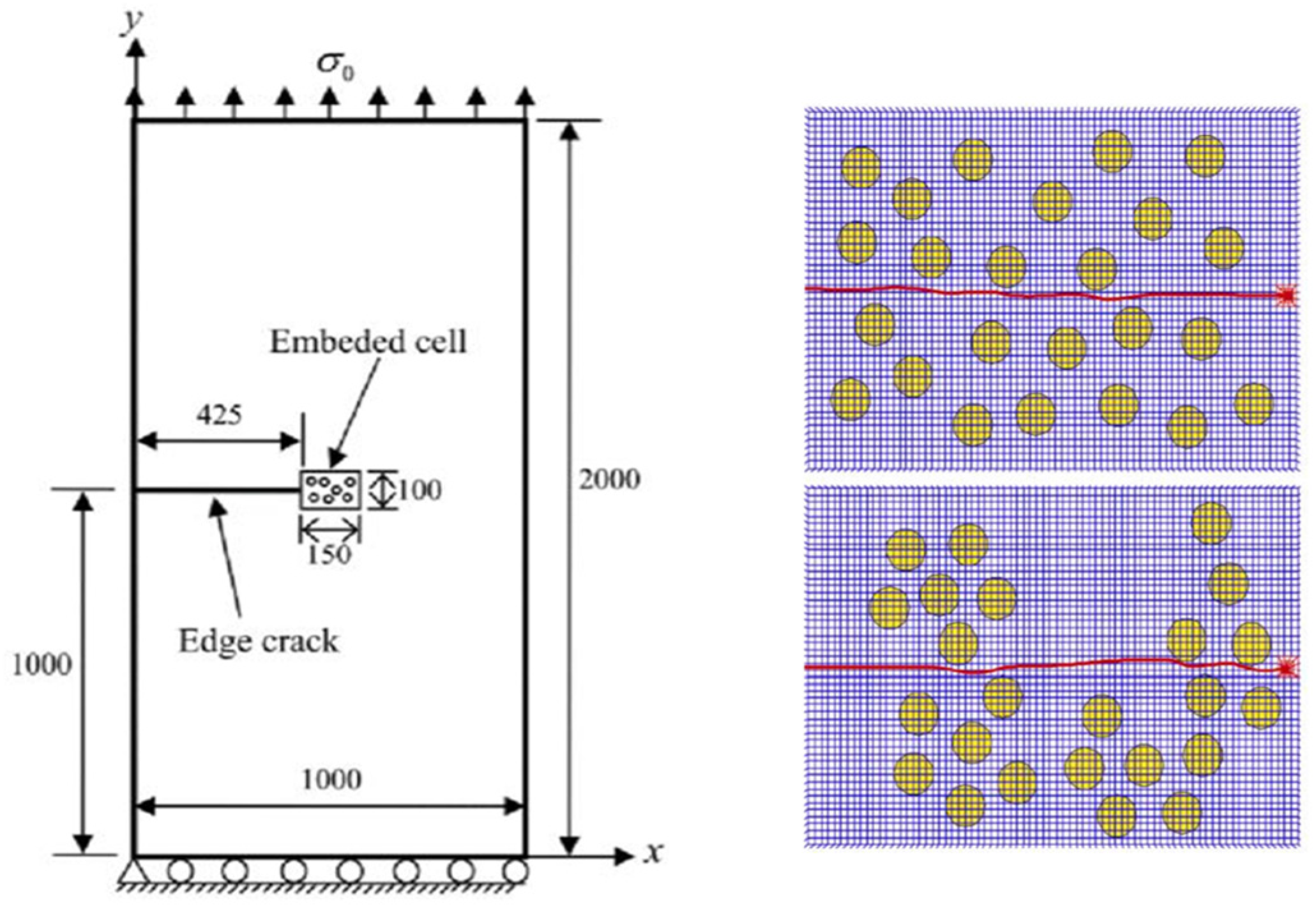
3.2. Numerical Examples of Heterogeneous Material Containing Inclusions

Composite materials commonly contain particulate inclusions within their internal structure, making them heterogeneous materials characterized by complex interfaces. This section validates the method for heterogeneous materials with inclusions and compares the results with the finite element results.

As shown in Figure 9, a rectangular plate of length h and width b has an edge crack of length a on one side. It contains a circular inclusion of radius R, whose center lies on the crack extension line, with a horizontal distance x between the inclusion center and the crack tip. The plate is subjected to uniform uniaxial tensile loads $\sigma =10\mathrm{MPa}$ on the upper and lower sides. The elastic moduli and Poisson’s ratios of the plate and inclusion are E₁, E₂ and, respectively. The data used in this example are as follows: h = 100 mm, b = 50 mm, R = 3 mm, x/R = 3, a = 25 mm, E₁ = 35 MPa, E₂ = 17.5 MPa, and ${\nu }_1={\nu }_2$ = 0.495.

Crack tips are meshed with CPS3 elements and refined to boost computational precision, while other regions use CPS4 elements. The mesh comprises 25,731 quadrilateral and 66 triangular elements, totaling 25,797 elements and 26,125 nodes. The stress intensity factors at crack tips are calculated by choosing integration domains of varying Rc/Rtip sizes, with the normalized factor defined as $K_0=\sigma \sqrt{\pi a}$.

In Figure 10, when the integration domain is small and excludes the inclusion or is large enough to fully contain it, both methods yield similar normalized stress intensity factors. However, when the integration domain intersects the inclusion, the stress intensity factors calculated by ABAQUS fluctuate significantly due to the unhandled interface derivative terms of the material parameter. This leads to inconsistent results across different domains, making accurate crack assessment difficult. In contrast, the method proposed in this paper ensures that the normalized stress intensity factor remains domain-independent, even when the domain intersects with the inclusion. Thus, the present method demonstrates unique advantages in handling heterogeneous materials with complex interfaces.

To analyze the influence of the inclusion’s properties on the stress intensity factor, the rectangular plate model with a circular inclusion and an edge crack shown in Figure 9a was selected. The aim was to study how inclusion parameters affect the stress intensity factor at the crack tip. The model dimensions were h = 100 mm, b = 50 mm, a = 25 mm, and R = 3 mm. The plate’s material properties were E₁ = 35 MPa and ${\nu }_1$ = 0.495, while the inclusion’s elastic modulus was E₂, with a Poisson’s ratio of ${\nu }_2$ = 0.495. By keeping the crack position and plate material properties constant and varying the inclusion’s horizontal position and elastic modulus, the study explores the influence of inclusion position and inclusion-to-plate modulus ratio on the stress intensity factor.

The normalized stress intensity factors at the crack tips were calculated for different inclusion-to-plate modulus ratios and inclusion positions. The normalized factor was the stress intensity factor when the plate has no inclusion. This paper analyzes two cases in which the inclusion’s elastic modulus is either larger or smaller than that of the plate. The results are shown in Figure 11, with the x-axis being the ratio of the inclusion center–crack tip distance to the inclusion radius.

As shown in Figure 11, when the inclusion’s elastic modulus exceeds the plate’s and approaches the crack tip, the normalized stress intensity factor decreases, indicating a crack-tip “blunting” effect. Conversely, when the inclusion’s modulus is lower than the plate’s and near the crack tip, the factor increases, showing a “sharpening” effect. Furthermore, the inclusion-to-plate modulus ratio significantly impacts the crack-tip stress intensity factor, with the “blunting” or “sharpening” effects becoming more pronounced as the ratio increases or decreases.

In actual composite materials, inclusions are usually multiple. As shown in Figure 12, in the two-dimensional rectangular plate of length h and width b, there are multiple circular inclusions with the radius R being randomly distributed. An edge crack of length a exists on one side of the plate, which is subjected to uniform uniaxial tensile loads $\sigma =10 \mathrm{MPa}$. The elastic modulus and Poisson’s ratio of the plate and inclusions are E₁, E₂ and ${\nu }_1$, ${\nu }_2$, respectively. The data used in this example are as follows: h = 100 mm, b = 50 mm, R = 3 mm, a = 25 mm, E₁ = 10⁵ MPa, ${\nu }_1$= 0.2, E₂ = 100 MPa, and ${\nu }_2$ = 0.2.

The crack tip was meshed with CPS3 elements and properly refined to enhance computational accuracy, while other regions used CPS4 elements. The entire mesh had 26,860 quadrilateral elements, 45 triangular elements, 26,905 elements in total, and 27,247 nodes. Integral domains with different Rc/Rtip ratios were chosen to calculate the stress intensity factor at the crack tip. The normalized factor was chosen as $K_0=\sigma \sqrt{\pi a}$.

Figure 13 compares the stress intensity factors from the present method and those from ABAQUS across different integration domains. When the domain is small, both methods yield similar results. As the domain grows and intersects the material interfaces, ABAQUS’s inability to handle the derivatives of material parameters means it fails to accurately reflect the crack-tip state. In contrast, the present method maintains stable values and satisfies domain-independence even when the integration domain crosses interfaces. This further highlights the advantage of the present method in solving the crack problems in heterogeneous materials with complex interfaces.

Furthermore, this paper analyzes the more realistic three-dimensional example. As shown in Figure 14, a cuboid of length h, width b, and height c contained a two-dimensional rectangular crack (length a, width c) and several cylindrical inclusions (base radius R, height c) were randomly distributed inside. The top and bottom surfaces of the cuboid were subjected to uniform uniaxial tensile loads $\sigma =10 \mathrm{MPa}$. The material parameters of the cuboid and inclusions were the same as those in the two-dimensional problem, specifically, h = 100 mm, b = 50 mm, c = 5 mm, a = 25 mm, and R = 3 mm.

The crack tip was meshed with wedge elements and properly refined to enhance computational accuracy, while other regions used hexahedral C3D8 elements. The entire mesh comprises 243 wedge elements, 94,963 hexahedral elements, 95,206 elements in total, and 110,694 nodes. Integral domains with different Rc/Rtip ratios were chosen to calculate the stress intensity factor at the mid-point of the three-dimensional crack front. The normalized factor was chosen as $K_0=\sigma \sqrt{\pi ac}$.

Figure 15 shows that, for three-dimensional heterogeneous materials with inclusions, the present method and ABAQUS results show a similar pattern to the two-dimensional case. When the domain intersects the inclusion, ABAQUS’s results make the crack assessment inaccurate. However, the present method maintains domain-independence for three-dimensional crack problems in materials with complex interfaces.

4. Summary and Conclusions

In this paper, an interaction integral method combined with the ABAQUS postprocessing routine technology is proposed for effectively calculating the crack fracture parameters for heterogeneous materials. Some conclusions are presented below:

(1)

The present method can be directly implemented within ABAQUS, and the computational results exhibit good accuracy, mesh convergence, and domain-independence.

(2)

For two-dimensional and three-dimensional models with inclusions, the results show that when the integration domain intersects the inclusions, the stress intensity factors calculated by ABAQUS fail to accurately reflect the crack-tip state, while the present method demonstrates good domain-independence, thereby expanding the practical application scope of ABAQUS.

(3)

The influence of the inclusion’s properties on the stress intensity factor was analyzed. The results show that high-modulus inclusions near the crack tip reduce the stress intensity factor. Conversely, low-modulus inclusions in the same area increase it.

(4)

The proposed method in this paper can be applied to heterogeneous materials with complex interfaces, such as particulate-reinforced composites and solid rocket motor grains. It can guide the crack conditions and crack propagation of practical components. In the future, it can also be combined with other software to provide guidance for engineering applications.

References

1. Chairi, M.; El Bahaoui, J.; Hanafi, I.; Cabrera, F.M.; Di Bella, G. Composite materials: A review of polymer and metal matrix composites, their mechanical characterization, and mechanical properties. In Next Generation Fiber-Reinforced Composites-New Insights; Intechopen: London, UK, 2023. [Google Scholar]
2. Janssen, M.; Zuidema, J.; Wanhill, R. Fracture Mechanics: Fundamentals and Applications, 2nd ed.; CRC Press: Boca Raton, FL, USA, 2017; p. 35. [Google Scholar]
3. Stern, M.; Becker, E.B.; Dunham, R.S. A contour integral computation of mixed-mode stress intensity. Int. J. Fract. 1976, 12, 359–368. [Google Scholar] [CrossRef]
4. Wang, Z.Y.; Yu, H.J.; Wang, Z.H. A local mesh replacement method for modeling near-interfacial crack growth in 2D composite structures. Theor. Appl. Fract. Mech. 2015, 75, 70–77. [Google Scholar] [CrossRef]
5. Li, Y.K.; Yu, H.J.; Guo, L.C.; Huang, K.; Bai, X.M. A new domain-independent interaction integral for three-dimensional non-homogeneous thermoelastic materials. Eng. Fract. Mech. 2020, 233, 107084. [Google Scholar] [CrossRef]
6. Wang, S.S.; Yau, J.F.; Corten, H.T. Three-dimensional stress fields of elastic interface cracks. J. Appl. Mech. 1980, 16, 247–259. [Google Scholar]
7. Nakamura, T. A mixed-mode crack analysis of rectilinear anisotropic solids using conservation laws of elasticity. Int. J. Fract. 1991, 58, 939–946. [Google Scholar]
8. Tabaza, O.; Okada, H.; Yusa, Y. A new approach of the interaction integral method with correction terms for cracks in three-dimensional functionally graded materials using the tetrahedral finite element. Theor. Appl. Fract. Mech. 2021, 115, 103065. [Google Scholar] [CrossRef]
9. Nahta, R.; Moran, B. Domain integrals for axisymmetric interface crack problems. Int. J. Solids Struct. 1993, 30, 2027–2040. [Google Scholar] [CrossRef]
10. Gosz, M.; Dolbow, J.; Moran, B. Domain integral formulation for stress intensity factor computation along curved three-dimensional interface cracks. Int. J. Solids Struct. 1998, 35, 1763–1783. [Google Scholar] [CrossRef]
11. Gosz, M.; Moran, B. An interaction energy integral method for computation of mixed-mode stress intensity factors along non-planar crack fronts in three dimensions. Eng. Fract. Mech. 2002, 69, 299–319. [Google Scholar] [CrossRef]
12. Nagashima, T.; Omoto, Y.; Tani, S. Stress intensity factor analysis of interface cracks using X-FEM. Int. J. Numer. Methods Eng. 2003, 56, 1151–1173. [Google Scholar] [CrossRef]
13. Sukumar, N.; Huang, Z.Y.; Prévost, J.H.; Suo, Z. Partition of unity enrichment for bimaterial interface cracks. Int. J. Numer. Methods Eng. 2004, 59, 1075–1102. [Google Scholar] [CrossRef]
14. Cisilino, A.P.; Ortiz, J.E. Three-dimensional boundary element assessment of a fibre/matrix interface crack under transverse loading. Comput. Struct. 2005, 83, 856–869. [Google Scholar] [CrossRef]
15. Ortiz, J.E.; Cisilino, A.P. Boundary element method for J-integral and stress intensity factor computations in three-dimensional interface cracks. Int. J. Fract. 2005, 133, 197–222. [Google Scholar] [CrossRef]
16. Merzbacher, M.J.; Horst, P. A model for interface cracks in layered orthotropic solids: Convergence of modal decomposition using the interaction integral method. Int. J. Numer. Methods Eng. 2009, 77, 1052–1071. [Google Scholar] [CrossRef]
17. Kim, J.H.; Paulino, G.H. T-stress, mixed-mode stress intensity factors, and crack initiation angles in functionally graded materials: A unified approach using the interaction integral method. Comput. Methods Appl. Mech. Eng. 2003, 192, 1463–1494. [Google Scholar] [CrossRef]
18. Yildirim, B. An equivalent domain integral method for fracture analysis of functionally graded materials under thermal stresses. J. Therm. Stress 2006, 29, 371–397. [Google Scholar] [CrossRef]
19. Duflot, M. The extended finite element method in thermoelastic fracture mechanics. Int. J. Numer. Methods Eng. 2008, 74, 827–847. [Google Scholar] [CrossRef]
20. Pathak, H. Crack interaction study in functionally graded materials (FGMs) using XFEM under thermal and mechanical loading environment. Mech. Adv. Mater. Struct. 2020, 27, 903–926. [Google Scholar] [CrossRef]
21. Zhu, S.; Yu, H.J.; Zhang, Y.B.; Yan, H.R.; Man, S.H.; Guo, L.C. Generalized dynamic domain-independent interaction integral in the transient fracture investigation of magneto-electro-elastic composites. Eng. Fract. Mech. 2023, 292, 109653. [Google Scholar] [CrossRef]
22. Guo, F.N.; Yu, H.J.; Zhang, Y.Y.; Guo, L.C. An interaction energy integral method for an interface crack in nonhomogeneous materials containing complex interfaces under thermal loading. Int. J. Solids Struct. 2023, 264, 112089. [Google Scholar] [CrossRef]
23. Yu, H.J.; Wu, L.Z.; Guo, L.C.; Du, S.Y.; He, Q.L. Investigation of mixed-mode stress intensity factors for nonhomogeneous materials using an interaction integral method. Int. J. Solids Struct. 2009, 46, 3710–3724. [Google Scholar] [CrossRef]
24. Yu, H.J.; Kuna, M. Interaction integral method for computation of crack parameters K–T–A review. Eng. Fract. Mech. 2021, 249, 107722. [Google Scholar] [CrossRef]
25. Williams, M.L. On the stress distribution at the base of a stationary crack. J. Appl. Mech. 1957, 24, 109–114. [Google Scholar] [CrossRef]
26. Gupta, M.; Alderliesten, R.C.; Benedictus, R. A review of T-stress and its effects in fracture mechanics. Eng. Fract. Mech. 2015, 134, 218–241. [Google Scholar] [CrossRef]
27. Moran, B.; Shih, C.F. Crack tip and associated domain integrals from momentum and energy balance. Eng. Fract. Mech. 1987, 27, 615–642. [Google Scholar] [CrossRef]
Figure 1. Definition of J integral.
Applsci 15 05827 g001
Figure 2. Simulation of crack propagation in complex interfacial materials using the interaction integral method [4].
Applsci 15 05827 g002
Figure 3. Flowchart of the calculation of interaction integral using the ABAQUS–Python postprocessing routine.
Applsci 15 05827 g003
Figure 4. Node and integration point locations in a two-dimensional isoparametric linear element.
Applsci 15 05827 g004
Figure 5. (a) Homogeneous rectangular plate with edge crack under unidirectional tensile load; (b) model meshes.
Applsci 15 05827 g005
Figure 6. (a) Homogeneous rectangular plate with a center-inclined crack under unidirectional tensile load; (b) model meshes.
Applsci 15 05827 g006
Figure 7. (a) The definition of mesh density; (b) the relative error for various refined meshes.
Applsci 15 05827 g007
Figure 8. The definition of integral domains.
Applsci 15 05827 g008
Figure 9. (a) Numerical example of two-dimensional heterogeneous materials with a single inclusion; (b) model meshes.
Applsci 15 05827 g009
Figure 10. Comparison of computational results between the present method and ABAQUS, providing a two-dimensional example with a single inclusion.
Applsci 15 05827 g010
Figure 11. The influence of elastic modulus of inclusions on normalized stress intensity factor.
Applsci 15 05827 g011
Figure 12. (a) Numerical example of two-dimensional heterogeneous materials with multiple inclusions; (b) model meshes.
Applsci 15 05827 g012
Figure 13. Comparison of the computational results between the present method and ABAQUS, showing a two-dimensional example with multiple inclusions.
Applsci 15 05827 g013
Figure 14. (a) A three-dimensional heterogeneous material with multiple inclusions; (b) model meshes.
Applsci 15 05827 g014
Figure 15. Comparison of computational results obtained by the present method and ABAQUS for a three-dimensional example with multiple inclusions.
Applsci 15 05827 g015