Article

Conditions for Guaranteeing Non-Overshooting Control of Nonlinear Systems with Full-State Constraints

School of Artificial Intelligence and Big Data, Hefei University, Hefei 230601, China
*
Author to whom correspondence should be addressed.
Appl. Sci. 2025, 15(11), 5816; https://doi.org/10.3390/app15115816
Submission received: 18 April 2025 / Revised: 15 May 2025 / Accepted: 15 May 2025 / Published: 22 May 2025

Abstract

:
In this paper, the problem of non-overshooting tracking control (NOTC) for a class of nonlinear systems with full-state constraints (FSCs) is studied. Firstly, this paper introduces the mapping constraint function to solve the FSC control problem and transform the controlled system into a new nonlinear system. Then, to obtain a closed-loop system that can solve the expression of tracking error, this paper transforms the n-order system into a system in which only the n-th subsystem is nonlinear by coordinate transformation, that is, subsystem 1 to subsystem n 1 are linear. Finally, according to the closed-loop system (CLS), the expressions of the first state of CLSs with n = 1 , n = 2 , n = 3 , and n 4 are solved, respectively. By analyzing these expressions, a wider range of conditions with NOTC are obtained. This algorithm obtains more conditions with non-overshooting. Compared with the existing results, the algorithm in this paper reduces the conservatism. Finally, the algorithm is applied to the single-link robot system, and the effectiveness of the algorithm is verified. That is, the algorithm in this paper not only makes all signals of the CLS bounded, but also makes the overshoot of the system zero.

1. Introduction

Since 1980s, scholars have paid more and more attention to nonlinear science, and nonlinear analysis in mathematics, nonlinear functional, and nonlinear dynamics in physics have developed rapidly [1]. At the same time, the theory of nonlinear systems has also developed vigorously [2,3,4,5,6,7], and more control theory experts have turned to research on nonlinear systems, and more engineers have tried to construct controllers with the theory of nonlinear systems, which has resulted in certain achievements. The feedback linearization method [8], backstepping method [9], sliding mode control method, and so on are proposed accordingly [10]. In order to ensure the security and improve the stability of the system, the main research result which is being focused on at present is the FSCs control method [11,12,13,14,15,16,17].
As a common state constraint method, FSC control has always been a research hotspot in the control field. At present, the algorithm combining barrier Lyapunov function (BLF), backstepping, and approximation control method is the main method used to solve the problem of FSCs control [11]. According to the definition, the value of the BLF tends to infinity as the function variable approaches the constraint boundary. When the BLF remains bounded under the action of the designed controller, the function variables will always remain within the constraint boundary; that is, the constraint is satisfied. This is also the key characteristic of the application of BLF to constraints control design.
However, the BLF also has some shortcomings. This algorithm directly constrains the state of the CLS rather than the state of the controlled system; that is, the constraint interval includes not only the states of the system, but also the virtual controllers. In this way, this method can be referred to as indirect FSC control. Therefore, the BLF control method needs to obtain the constraint interval through complicated calculations. To solve the shortage of BLF, reference [18] proposed a mapping logarithmic constraint function to solve the problem of FSCs control. The constraint interval in this method only contains the system state. Therefore, reasonable constraint parameters or functions can be directly designed according to the actual needs of the state. This method can be referred to as direct FSC control.
Both the BLF and the mapping logarithmic constraint function use constraint parameters or functions to play a security role in the system. For example, if the overshoot of the system is too large, we can reduce the overshoot of the system by designing constraint parameters or functions. However, due to the inherent characteristics of its method, the constraint parameters or functions cannot be designed to be zero, which means the overshoot of the system is unable to reach zero; that is, the NOTC cannot be realized. However, the NOTC is very useful in practical applications, and in some applications [19], it is also required that the control method can achieve the result with NOTC, such as the temperature control of sintering furnace [20], missile launch, attitude control of flight control system and welding operation, and so on. Therefore, it is necessary to study the NOTC.
At present, the research results of NOTC are mainly aimed at linear systems [21,22,23,24,25], and there are very few studies which focus on nonlinear systems. For the nonlinear strict-feedback system, an improved controller was designed for the first time based on backstepping reference [19], and thus a linear CLS was obtained. Reference [26] pointed out that reference [19] mainly used backstepping technology to construct control law and obtain a chain CLS, in which the first CLS state was a tracking error. By selecting design parameters, the initial values of all CLS states were guaranteed to be negative, so that all CLS states remain negative in the convergence process. This method abandons other NOTC conditions that guarantee the tracking error will be negative. Therefore, this kind of thinking is quite conservative. Then, reference [26] used the backstepping method to design an improved controller, and the CLS was the same as the linear CLS in reference [19], and then the conditions of NOTC were discussed based on the Laplace transform. Compared with references [19], reference [26] obtained wider conditions of non-overshooting, which reduced the conservatism. Reference [27] studied the problem of output tracking with non-overshooting of a feedback linearization nonlinear system, and proposed a controller design program using feedback linearization and global coordinate transformation technology. Compared with references [19,26], the nonlinear function in the controlled system in reference [27] not only needs to be assumed to be known, but also needs to be bounded, so this increases the conservatism. In addition, references [28,29,30,31] have studied the problem of non-overshooting control of nonlinear systems.
It is worth mentioning that in recent years, there have been some breakthroughs in NOTC of nonlinear systems. Reference [32] first proposed the mean-non-overshooting tracking control design for stochastic strict-feedback nonlinear systems. The obtained results ensure that the overshoot can be adjusted to be as small as possible under the condition that all the states of the CLS remain bounded. At the same time, reference [33] designs a finite-time control algorithm for nonlinear strict-feedback systems, which makes the overshoot arbitrarily small. However, compared with the NOTC algorithm, this method fails to achieve the control goal of non-overshooting, thus reducing the accuracy of non-overshooting.
The method in this paper is mainly aimed at a class of nonlinear systems, and the problem of NOTC with FSCs is studied. Compared with the existing related literature, this paper has the following differences:
(1)
Compared with the BLF [11], this paper uses the mapping constraint function, which is a direct constraint method, thus reducing the calculation burden of constraint parameters.
(2)
On the basis of FSCs, the problem of NOTC is discussed, which makes the FSCs method realize the result of NOTC. Compared with the existing FSCs method [11,12,13,14,15,16,17], the overshoot of tracking error can be 0.
(3)
Regarding NOTC, because the expression of tracking error is adopted in this paper, a wider range of non-overshooting in conditions can be obtained compared with that of the existing methods [19,26,27,32,33], which reduces the conservatism.
(4)
The most difficult problem that arises when designing the algorithm in this paper relates to obtaining a CLS that can solve the expression of tracking error. To obtain a CLS that can easily calculate the expression of tracking error, this paper needs to convert the situation in which each subsystem is nonlinear into a system that only contains the n-th subsystem as nonlinear (such as (25)). Otherwise, it is difficult to calculate the expression of tracking error for the obtained CLS. Then, this algorithm provides a method to transform the controlled system into a system that is simpler to deal with. Compared with the existing control results with NOTC, this algorithm is simpler.
The layout of the rest of this article is as follows: The problem formulation is given in Section 2. The full-state constraints control and control design are shown in Section 3. The NOTC is written in Section 4. An example is given in Section 5, and the conclusions of this paper are provided in Section 6.

2. Problem Formulation

Consider nonlinear systems as
ξ ˙ i = ξ i + 1 + f i ( ξ 1 , · · · , ξ i ) , i = 1 , · · · , n 1 , ξ ˙ n = u + f n ( ξ 1 , · · · , ξ n ) , y = ξ 1 ,
where ξ = [ ξ 1 , · · · , ξ n ] T , u R and y R are the system states, the system input and system output, respectively. Define ξ ¯ i = [ ξ 1 , · · · , ξ i ] T ( i = 1 , · · · , n ). f 1 ( · ) , · · · , f n ( · ) are nonlinear smooth known functions.
The expression for the tracking error e ( t ) in this article is as follows:
e ( t ) = y ( t ) y 0 ( t ) ,
where y 0 ( t ) is a smooth and bounded reference signal with n differentiable times.
According to reference [19], the NOTC means that the sign of the tracking error e ( t ) in t [ 0 , + ] is constant; that is,
e ( t ) 0 o r e ( t ) 0 .
Therefore, the control goal of this paper is to use the design state constraint non-overshoot controller, and the controlled system meets the following conclusions:
(1)
All signals of the CLS are bounded, and the tracking error satisfies lim t e ( t ) = 0 ;
(2)
The tracking error e ( t ) satisfies the condition of NOTC; that is, e ( t ) always keeps e ( t ) 0 or e ( t ) 0 ;
(3)
The constraint property of the BLFs is not violated; that is, the system state ξ i ( i = 1 , · · · , n ) satisfies the following constraints
k i 1 < ξ i ( t ) < k i 2 ,
where k i 1 < 0 and k i 2 > 0 are constraint parameters.
Lemma 1.
Define the following two functions.
Y 1 ( t ) = ln y 1 ( t ) k 1 k 2 y 1 ( t ) , Y 2 ( t ) = ln y 2 ( t ) k 1 k 2 y 2 ( t ) ,
where k 1 < 0 and k 2 > 0 are constants, and the functions y 1 ( t ) and y 2 ( t ) satisfy k 1 < y 1 ( t ) < k 2 and k 1 < y 2 ( t ) < k 2 , respectively.
If lim t ( Y 1 ( t ) Y 2 ( t ) ) = 0 , then
lim t ( y 1 ( t ) y 2 ( t ) ) = 0 .
Proof. 
Define Y ( t ) = Y 1 ( t ) Y 2 ( t ) . According to (5), we have
Y ( t ) = ln y 1 ( t ) k 1 k 2 y 1 ( t ) ln y 2 ( t ) k 1 k 2 y 2 ( t ) = ln ( y 1 ( t ) k 1 ) ( k 2 y 2 ( t ) ) ( k 2 y 1 ( t ) ) ( y 2 ( t ) k 1 ) .
From lim t ( Y 1 ( t ) Y 2 ( t ) ) = 0 , k 1 < y 1 ( t ) < k 2 and k 1 < y 2 ( t ) < k 2 , we have the following derivation
lim t Y ( t ) = 0 lim t ln ( y 1 ( t ) k 1 ) ( k 2 y 2 ( t ) ) ( k 2 y 1 ( t ) ) ( y 2 ( t ) k 1 ) = 0 lim t ( y 1 ( t ) k 1 ) ( k 2 y 2 ( t ) ) ( k 2 y 1 ( t ) ) ( y 2 ( t ) k 1 ) = 1 lim t ( y 1 ( t ) y 2 ( t ) ) ( k 2 k 1 ) = 0 lim t ( y 1 ( t ) y 2 ( t ) ) = 0 .

3. Full-State Constraints Control and Control Design

To solve the FSCs problem of the system (1), the following constraint function is introduced.
x i = ln ξ i ( t ) k i 1 k i 2 ξ i ( t ) , i = 1 , · · · , n ,
where k i 1 < 0 and k i 2 > 0 are constraint parameters.
From (5), we get
x i ˙ = k i 2 k i 1 ( ξ i k i 1 ) ( k i 2 ξ i ) ξ ˙ i .
Substituting (1) and the inverse functions of (9) into (10), the system is given as
x ˙ i = F i ( x ¯ i , x i + 1 ) , i = 1 , · · · , n 1 , x ˙ n = g n ( x n ) u + F n ( x ¯ n ) ,
where
F i ( x ¯ i , x i + 1 ) = g i ( x i ) ( f i ( k 12 e x 1 + k 11 1 + e x 1 , · · · , k i 2 e x i + k i 1 1 + e x i ) + k ( i + 1 ) 2 e x i + 1 + k ( i + 1 ) 1 1 + e x i + 1 ) , i = 1 , · · · , n 1 ,
g i ( x i ) = ( 1 + e x i ) 2 ( k i 2 k i 1 ) e x i , i = 1 , · · · , n ,
F n ( x ¯ n ) = g n ( x n ) f n ( k 12 e x 1 + k 11 1 + e x 1 , · · · , k n 2 e x n + k n 1 1 + e x n ) .
Remark 1.
According to (11), we can design the controller according to the algorithm in Reference [18]. However, it is a pity that the CLS obtained in this way is more complicated. As a result, it is difficult to find the expression of tracking error, and then it is impossible to get a wider range of conditions with NOTC.
Therefore, this paper has to make the following transformation.
Define θ 1 = x 1 and θ 2 = θ ˙ 1 , then
θ ˙ 2 = θ ¨ 1 = a 2 ( x ¯ 2 ) + b 2 ( x ¯ 3 ) ,
where
a 2 ( x ¯ 2 ) = F 1 ( x ¯ 2 ) x 1 F 1 ( x ¯ 2 ) , b 2 ( x ¯ 3 ) = F 1 ( x ¯ 2 ) x 2 F 2 ( x ¯ 3 ) .
Define θ 3 = θ ˙ 2 , then
θ ˙ 3 = θ ¨ 2 = a 3 ( x ¯ 3 ) + b 3 ( x ¯ 4 ) ,
where
b 3 ( x ¯ 4 ) = b 2 ( x ¯ 3 ) x 3 f 3 ( x ¯ 4 ) , a 3 ( x ¯ 3 ) = j = 1 2 [ a 2 ( x ¯ 2 ) x j F j ( x ¯ j + 1 ) + b 2 ( x ¯ 3 ) x j F j ( x ¯ j + 1 ) ] .
Define θ 4 = θ ˙ 3 , then
θ ˙ 4 = θ ¨ 3 = a 4 ( x ¯ 4 ) + b 4 ( x ¯ 5 ) ,
where
b 4 ( x ¯ 5 ) = b 3 ( x ¯ 4 ) x 4 F 4 ( x ¯ 5 ) , a 4 ( x ¯ 4 ) = j = 1 3 [ a 3 ( x ¯ 3 ) x j F j ( x ¯ j + 1 ) + b 3 ( x ¯ 4 ) x j F j ( x ¯ j + 1 ) ] .
Similarly, define θ i = θ ˙ i 1 ( i = 5 , · · · , n 1 ). We have
θ ˙ i = θ ¨ i 1 = a i ( x ¯ i ) + b i ( x ¯ i + 1 ) ,
where
b i ( x ¯ i + 1 ) = b i 1 ( x ¯ i ) x i f i ( x ¯ i + 1 ) , a i ( x ¯ i ) = j = 1 i 1 [ a i 1 ( x ¯ i 1 ) x j f j ( x ¯ j + 1 ) + b i 1 ( x ¯ i ) x j f j ( x ¯ j + 1 ) ] .
Similarly, define θ n = θ ˙ n 1 . Then, we have
θ ˙ n = θ ¨ n 1 = a n ( x ¯ n ) + b n ( x ¯ n ) u ,
where
b n ( x ¯ n ) = b n 1 ( x ¯ n ) x n g n ( x n ) , a n ( x ¯ n ) = j = 1 n 1 [ a n 1 ( x ¯ n 1 ) x j F j ( x ¯ j + 1 ) + b n 1 ( x ¯ n ) x j F j ( x ¯ j + 1 ) ] + b n 1 ( x ¯ n ) x n F n ( x ¯ n ) .
According to (11)–(24), we can summarize the following system
θ ˙ i = θ i + 1 , i = 1 , · · · , n 1 , θ ˙ n = a n ( x ¯ n ) + b n ( x ¯ n ) u .
Next, the controller is designed based on backstepping. First, we define the following coordinate transformation
η 1 = θ 1 Y 0 , η i = θ i α i 1 , i = 2 , · · · , n ,
where Y 0 = ln y 0 ( t ) k 11 k 12 y 0 ( t ) , and the constraint parameters k 11 and k 12 need to satisfy k 11 < y 0 ( t ) < k 12 , and α i 1 is the virtual controller to be designed. According to the process of designing the controller by backstepping, the virtual controllers and the controller u are designed as follows
α 1 = ε 1 η 1 + Y ˙ 0 , α i = ε i η i + α ˙ i 1 , i = 2 , · · · , n 1 , u = 1 b n ( x ¯ n ) [ ε n η n + α ˙ n 1 a n ( x ¯ n ) ] ,
where ε 1 > 1 2 , ε i > 1 ( i = 2 , · · · , n 1 ) and ε n > 1 2 is the control gain parameter. According to the above design process, the definition of b n ( x ¯ n ) satisfies b n ( x ¯ n ) 0 .
Let Lyapunov function V = 1 2 Σ j = 1 n η j 2 . Substituting the designed virtual controllers and controller (23) into V ˙ , then
V ˙ n = j = 1 n ε j η j 2 + j = 1 n 1 η j η j + 1 ( ε 1 1 2 ) η 1 2 j = 2 n 1 ( ε j 1 ) η j 2 ( ε n 1 2 ) η n 2 ρ V n ,
where ρ = min { ( 2 c 1 1 ) , ( 2 c i 2 ) , ( 2 c n 1 ) } ( i = 2 , · · · , n 1 ).
Therefore, signals η 1 , · · · , η n are bounded, and η 1 , · · · , η n satisfy lim t η 1 = 0 , · · · , lim t η n = 0 . According to Lemma 1, lim t e ( t ) = 0 , and the signals θ 1 , · · · , θ n are bounded. From the definition of θ 1 , · · · , θ n , signals x 1 , F 1 ( x ¯ 2 ) , · · · , F n 1 ( x ¯ n ) are bounded.
Since F 1 ( x ¯ 2 ) is a smooth function, there is at least one point ϵ 1 ( ϵ 1 ( min ( 0 , x 2 ) , max ( 0 , x 2 ) ) ) to make
F 1 ( x 1 , x 2 ) F 1 ( x 1 , 0 ) = F 1 ( x 1 , x 2 ) x 2 | x 2 = ϵ 1 ( x 2 0 ) .
Then, x 2 ( t ) is also bounded. Similarly, we can determine that x 3 ( t ) , · · · , x n ( t ) are bounded. According to (5), the FSCs have not been violated. Therefore, k i 1 < ξ i ( t ) < k i 2 , ( i = 1 , · · · , n ).
Remark 2.
According to (28), we can get
| η i | 2 | V n ( 0 ) | e ρ t , i = 1 , · · · , n .
From the above formula, we can see that the amplitude of the closed-loop system will increase with the increase in the initial value V n ( 0 ) . And with the increase in the parameter ρ, the convergence speed of the closed-loop system increases.

4. Non-Overshooting Tracking Control

In this section, we will calculate the expressions of tracking error through a CLS. Then, the non-overshooting control conditions with system orders of n = 1 , n = 2 , n = 3 , and n 4 are obtained, respectively.
Combining (25)–(27), we can obtain the following CLS.
η ˙ 1 = ε 1 η 1 + η 2 , η ˙ i = ε i η i + η i + 1 , i = 2 , · · · , n 1 , η ˙ n = ε n η n ,
We will analyze the control problem with NOTC conditions according to the following situations.
(1)
The situation when n = 1 .
The CLS (30) is a first-order system η ˙ 1 = ε 1 η 1 . This subsystem is integrated along [ 0 , t ] , and η 1 ( t ) is obtained as
η 1 ( t ) = η 1 ( 0 ) e ε 1 t ,
where η 1 ( 0 ) is the initial value of η 1 ( t ) .
Then, we obtain
η 1 ( 0 ) 0 η 1 ( t ) 0 ,
From (2), (9), (26) and Y 0 = ln y 0 ( t ) k 11 k 12 y 0 ( t ) , we have
η 1 ( t ) 0 θ 1 ( t ) Y 0 ( t ) 0 ln ξ 1 ( t ) k 11 k 12 ξ 1 ( t ) ln y 0 ( t ) k 11 k 12 y 0 ( t ) 0 ( ξ 1 ( t ) k 11 ) ( k 12 y 0 ( t ) ) ( k 12 ξ 1 ( t ) ) ( y 0 ( t ) k 11 ) 1 ( k 12 k 11 ) ( y ( t ) y 0 ( t ) ) 0 .
Since k 12 k 11 > 0 , then
y ( t ) y 0 ( t ) 0 e ( t ) 0 .
Combining (32)–(34), we get
η 1 ( 0 ) 0 e ( t ) 0 .
Similarly, the following result is also true
η 1 ( 0 ) 0 e ( t ) 0 .
To sum up, we can obtain the following theorem.
Theorem 1.
For the first-order system (1), we can make all the signals of the CLS bounded by designing the controller (27), and the tracking error satisfies lim t e ( t ) = 0 . At the same time, the NOTC needs to satisfy one of the conditions (35) and (36).
(2)
The situation when n = 2 .
The CLS is a second-order system η ˙ 1 = ε 1 η 1 + η 2 and η ˙ 2 = ε 2 η 2 .
We will divide it into two cases to obtain the condition of non-overshooting.
Case 1:  ε 1 ε 2 .
We first solve the integral of η 2 along [ 0 , t ] is η 2 ( t ) = η 2 ( 0 ) e ε 2 t , where η 2 ( 0 ) is the initial value of η 2 ( t ) . Then, substituting η 2 ( t ) into η ˙ 1 = ε 1 η 1 + η 2 to get
η ˙ 1 = ε 1 η 1 + η 2 ( 0 ) e ε 2 t .
This subsystem is integrated along [ 0 , t ] , and η 1 ( t ) is obtained as
η 1 ( t ) = [ η 1 ( 0 ) η 2 ( 0 ) ε 1 ε 2 ] e ε 1 t + η 2 ( 0 ) ε 1 ε 2 e ε 2 t ,
By analyzing (38), we can get the following conditions
η 1 ( 0 ) 0 , η 2 ( 0 ) 0 , ε 1 η 2 ( 0 ) η 1 ( 0 ) + ε 2 , ε 2 η 2 ( 0 ) η 1 ( 0 ) , η 1 ( t ) 0 ,
η 1 ( 0 ) 0 , ε 1 < ε 2 , η 1 ( 0 ) η 2 ( 0 ) ε 1 ε 2 , η 1 ( t ) 0 .
According to (33) and (34), the following two conditions with non-overshooting can be obtained.
η 1 ( 0 ) 0 , η 2 ( 0 ) 0 , ε 1 η 2 ( 0 ) η 1 ( 0 ) + ε 2 , ε 2 η 2 ( 0 ) η 1 ( 0 ) , e ( t ) 0 ,
η 1 ( 0 ) 0 , ε 1 < ε 2 , η 1 ( 0 ) η 2 ( 0 ) ε 1 ε 2 , e ( t ) 0 .
Case 2:  ε 1 = ε 2 = ε .
According to ε 1 = ε 2 = ε and (30), we solve η ˙ 1 = ε η 1 + η 2 as follows
η 1 ( t ) = [ η 1 ( 0 ) + η 2 ( 0 ) t ] e ε t .
By analyzing Equation (43), we can obtain the following conditions
η 1 ( 0 ) 0 , η 2 ( 0 ) 0 , η 1 ( t ) 0 ,
η 1 ( 0 ) 0 , η 2 ( 0 ) 0 , η 1 ( t ) 0 .
According to (33) and (34), the following two conditions with non-overshooting can be obtained.
η 1 ( 0 ) 0 , η 2 ( 0 ) 0 , e ( t ) 0 ,
η 1 ( 0 ) 0 , η 2 ( 0 ) 0 , e ( t ) 0 .
To sum up, we can obtain the following theorem.
Theorem 2.
For the second-order system (1), we constrain the controller (27) so that all signals of the CLS are bounded, and the tracking error satisfies lim t e ( t ) = 0 , and the states constraint is not violated. At the same time, NOTC can result in the following two situations, according to the control gain:
(1) 
If ε 1 ε 2 , then NOTC can satisfy (41) or (42);
(2) 
If ε 1 = ε 2 , then NOTC can satisfy (46) or (47).
(3)
The situation when  n = 3 .
The CLS is a third-order system; that is, η ˙ 1 = ε 1 η 1 + η 2 and η ˙ 2 = ε 2 η 2 + η 3 and η ˙ 3 = ε 3 η 3 . We will divide it into several cases to obtain the conditions of NOTC.
Case 1:  ε 1 ε 2 ε 3 .
Then, we obtain the expressions of η 3 ( t ) and η 2 ( t ) as follows
η 3 ( t ) = η 3 ( 0 ) e ε 3 t , η 2 ( t ) = [ η 2 ( 0 ) η 3 ( 0 ) ε 2 ε 3 ] e ε 2 t + η 3 ( 0 ) ε 2 ε 3 e ε 3 t ,
where η 3 ( 0 ) is the initial value of η 3 ( t ) .
Then, substituting (48) into η ˙ 1 = ε 1 η 1 + η 2 to get
η ˙ 1 = ε 1 η 1 + [ η 2 ( 0 ) η 3 ( 0 ) ε 2 ε 3 ] e ε 2 t + η 3 ( 0 ) ε 2 ε 3 e ε 3 t .
This subsystem is integrated along [ 0 , t ] , and η 1 ( t ) is obtained as
η 1 ( t ) = [ η 1 ( 0 ) η 2 ( 0 ) ε 1 ε 2 + η 3 ( 0 ) ( ε 1 ε 2 ) ( ε 2 ε 3 ) η 3 ( 0 ) ( ε 1 ε 3 ) ( ε 2 ε 3 ) ] e ε 1 t + [ η 2 ( 0 ) ε 1 ε 2 η 3 ( 0 ) ( ε 1 ε 2 ) ( ε 2 ε 3 ) ] e ε 2 t + η 3 ( 0 ) ( ε 1 ε 3 ) ( ε 2 ε 3 ) e ε 3 t ,
we obtain the following conditions by analyzing (50).
η 1 ( 0 ) η 2 ( 0 ) ε 1 ε 2 η 3 ( 0 ) ( ε 1 ε 2 ) ( ε 1 ε 3 ) , η 2 ( 0 ) ( ε 1 ε 2 ) ( ε 2 ε 3 ) η 3 ( 0 ) ( ε 1 ε 3 ) ( ε 2 ε 3 ) , η 3 ( 0 ) ( ε 1 ε 3 ) ( ε 2 ε 3 ) 0 , η 1 ( t ) 0 .
η 1 ( 0 ) η 2 ( 0 ) ε 1 ε 2 η 3 ( 0 ) ( ε 1 ε 2 ) ( ε 1 ε 3 ) , η 2 ( 0 ) ε 1 ε 2 η 3 ( 0 ) ( ε 1 ε 2 ) ( ε 2 ε 3 ) , η 2 ( 0 ) ε 1 ε 2 η 3 ( 0 ) ( ε 1 ε 2 ) ( ε 1 ε 3 ) , ε 2 < ε 3 , η 1 ( t ) 0 .
η 1 ( 0 ) η 3 ( 0 ) ε 1 ε 2 η 3 ( 0 ) ( ε 1 ε 2 ) ( ε 1 ε 3 ) , η 3 ( 0 ) ( ε 1 ε 3 ) ( ε 2 ε 3 ) 0 , η 2 ( 0 ) ε 1 ε 2 η 3 ( 0 ) ( ε 1 ε 3 ) ( ε 2 ε 3 ) , ε 3 < ε 2 , η 1 ( t ) 0 .
η 1 ( 0 ) η 2 ( 0 ) ε 1 ε 2 η 3 ( 0 ) ( ε 1 ε 2 ) ( ε 2 ε 3 ) , η 1 ( 0 ) η 2 ( 0 ) ε 1 ε 2 η 3 ( 0 ) ( ε 1 ε 2 ) ( ε 1 ε 3 ) , η 2 ( 0 ) ε 1 ε 2 η 3 ( 0 ) ( ε 1 ε 2 ) ( ε 2 ε 3 ) , ε 1 < ε 3 , η 1 ( t ) 0 .
η 2 ( 0 ) ε 1 ε 2 η 3 ( 0 ) ( ε 1 ε 2 ) ( ε 2 ε 3 ) , η 1 ( 0 ) η 2 ( 0 ) ε 1 ε 2 η 3 ( 0 ) ( ε 1 ε 2 ) ( ε 2 ε 3 ) , η 3 ( 0 ) ( ε 1 ε 3 ) ( ε 2 ε 3 ) 0 , ε 3 < ε 1 , η 1 ( t ) 0 .
η 3 ( 0 ) ( ε 1 ε 3 ) ( ε 2 ε 3 ) 0 , η 1 ( 0 ) η 2 ( 0 ) ε 1 ε 2 η 3 ( 0 ) ( ε 1 ε 2 ) ( ε 1 ε 3 ) , η 1 ( 0 ) η 3 ( 0 ) ( c 1 c 3 ) ( c 2 c 3 ) , ε 1 < ε 2 , η 1 ( t ) 0 .
η 3 ( 0 ) ( ε 1 ε 3 ) ( ε 2 ε 3 ) 0 , η 2 ( 0 ) η 3 ( 0 ) ε 2 ε 3 , η 1 ( 0 ) η 3 ( 0 ) ( ε 1 ε 3 ) ( ε 2 ε 3 ) , ε 2 < ε 1 . η 1 ( t ) 0 .
According to (33) and (34), η 1 ( t ) 0 e ( t ) 0 . Therefore, any of inequalities (51)–(57) can satisfy that the tracking error satisfies e ( t ) 0 . Then, inequalities (51)–(57) are NOTC conditions.
In the same way, we can obtain the following conditions by analyzing (50)
η 1 ( 0 ) η 2 ( 0 ) ε 1 ε 2 η 3 ( 0 ) ( ε 1 ε 2 ) ( ε 1 ε 3 ) , η 2 ( 0 ) ( ε 1 ε 2 ) ( ε 2 ε 3 ) η 3 ( 0 ) ( ε 1 ε 3 ) ( ε 2 ε 3 ) , η 3 ( 0 ) ( ε 1 ε 3 ) ( ε 2 ε 3 ) 0 . η 1 ( t ) 0 .
η 1 ( 0 ) η 2 ( 0 ) ε 1 ε 2 η 3 ( 0 ) ( ε 1 ε 2 ) ( ε 1 ε 3 ) , η 2 ( 0 ) ε 1 ε 2 η 3 ( 0 ) ( ε 1 ε 2 ) ( ε 2 ε 3 ) , η 2 ( 0 ) ε 1 ε 2 η 3 ( 0 ) ( ε 1 ε 2 ) ( ε 1 ε 3 ) , ε 2 < ε 3 , η 1 ( t ) 0 .
η 1 ( 0 ) η 3 ( 0 ) ε 1 ε 2 η 3 ( 0 ) ( ε 1 ε 2 ) ( ε 1 ε 3 ) , η 3 ( 0 ) ( ε 1 ε 3 ) ( ε 2 ε 3 ) 0 , η 2 ( 0 ) ε 1 ε 2 η 3 ( 0 ) ( ε 1 ε 2 ) ( ε 1 ε 3 ) , ε 3 < ε 2 , η 1 ( t ) 0 .
η 1 ( 0 ) η 2 ( 0 ) ε 1 ε 2 η 3 ( 0 ) ( ε 1 ε 2 ) ( ε 2 ε 3 ) , η 1 ( 0 ) η 2 ( 0 ) ε 1 ε 2 η 3 ( 0 ) ( ε 1 ε 2 ) ( ε 1 ε 3 ) , η 2 ( 0 ) ε 1 ε 2 η 3 ( 0 ) ( ε 1 ε 2 ) ( ε 2 ε 3 ) , ε 1 < ε 3 , η 1 ( t ) 0 .
η 2 ( 0 ) ε 1 ε 2 η 3 ( 0 ) ( ε 1 ε 2 ) ( ε 2 ε 3 ) , η 1 ( 0 ) η 2 ( 0 ) ε 1 ε 2 η 3 ( 0 ) ( ε 1 ε 2 ) ( ε 2 ε 3 ) , η 3 ( 0 ) ( ε 1 ε 3 ) ( ε 2 ε 3 ) 0 , ε 3 < ε 1 , η 1 ( t ) 0 .
η 3 ( 0 ) ( ε 1 ε 3 ) ( ε 2 ε 3 ) 0 , η 1 ( 0 ) η 2 ( 0 ) ε 1 ε 2 η 3 ( 0 ) ( ε 1 ε 2 ) ( ε 1 ε 3 ) , η 1 ( 0 ) η 3 ( 0 ) ( ε 1 ε 2 ) ( ε 2 ε 3 ) , ε 1 < ε 2 , η 1 ( t ) 0 .
η 3 ( 0 ) ( ε 1 ε 3 ) ( ε 2 ε 3 ) 0 , η 2 ( 0 ) η 3 ( 0 ) ( ε 2 ε 3 ) , η 1 ( 0 ) η 3 ( 0 ) ( ε 1 ε 3 ) ( ε 2 ε 3 ) , ε 2 < ε 1 , η 1 ( t ) 0 .
Similarly, according to (33) and (34), η 1 ( t ) 0 e ( t ) 0 . Therefore, any of the inequalities (58)–(64) can satisfy that the tracking error satisfies e ( t ) 0 . Then, inequalities (58)–(64) are NOTC conditions.
Case 2:  ε 1 = ε 2 = ε ε 3 .
In this case, we can determine the expression of ε 3 ( t ) and ε 2 ( t ) as shown in (48). According to ε 1 = ε 2 = ε , we integrate η ˙ 1 = ε η 1 + η 2 along [ 0 , t ] , then η 1 ( t ) is
η 1 ( t ) = [ η 1 ( 0 ) η 3 ( 0 ) ( ε ε 3 ) 2 + ( η 2 ( 0 ) η 3 ( 0 ) ε ε 3 ) t ] e ε t + η 3 ( 0 ) ( ε ε 3 ) 2 e ε 3 t .
we obtain the following conditions by analyzing (65)
η 1 ( 0 ) η 3 ( 0 ) ( ε ε 3 ) 2 , η 2 ( 0 ) η 3 ( 0 ) ε ε 3 , η 3 ( 0 ) 0 , η 1 ( t ) 0 .
η 1 ( 0 ) 0 , η 2 ( 0 ) η 3 ( 0 ) ε ε 3 , η 3 ( 0 ) 0 , ε < ε 3 , η 1 ( t ) 0 .
η 1 ( 0 ) 0 , η 2 ( 0 ) η 3 ( 0 ) ε ε 3 , η 3 ( 0 ) 0 , ε > ε 3 . η 1 ( t ) 0 .
η 1 ( 0 ) η 3 ( 0 ) ( ε ε 3 ) 2 , η 2 ( 0 ) η 3 ( 0 ) ε ε 3 , η 3 ( 0 ) 0 , ε < ε 3 , η 1 ( t ) 0 .
According to (33) and (34), η 1 ( t ) 0 e ( t ) 0 . Therefore, any of the inequalities (66)–(69) can indicate that the tracking error satisfies e ( t ) 0 . Then, inequalities (66)–(69) are NOTC conditions.
In the same way, we can obtain the following conditions by analyzing (65)
η 1 ( 0 ) η 3 ( 0 ) ( ε ε 3 ) 2 , η 2 ( 0 ) η 3 ( 0 ) ε ε 3 , η 3 ( 0 ) 0 , η 1 ( t ) 0 .
η 1 ( 0 ) 0 , η 2 ( 0 ) η 3 ( 0 ) ε ε 3 , η 3 ( 0 ) 0 , ε < ε 3 , η 1 ( t ) 0 .
η 1 ( 0 ) η 3 ( 0 ) ( ε ε 3 ) 2 , η 2 ( 0 ) η 3 ( 0 ) ε ε 3 , η 3 ( 0 ) 0 , ε < ε 3 , η 1 ( t ) 0 .
η 1 ( 0 ) 0 , η 2 ( 0 ) η 3 ( 0 ) ε ε 3 , η 3 ( 0 ) 0 , ε 3 < ε . η 1 ( t ) 0 .
According to (33) and (34), η 1 ( t ) 0 e ( t ) 0 . Therefore, any of the inequalities (70)–(73) can indicate that the tracking error satisfies e ( t ) 0 . Then, inequalities (70)–(73) are NOTC conditions.
Case 3:  ε 1 ε 2 = ε 3 = ε .
According to (30), we integrate this subsystem along [ 0 , t ] , η 3 ( t ) is obtained as (48), and η 2 ( t ) and η 1 ( t ) can be written as
η 2 ( t ) = ( η 2 ( 0 ) + η 3 ( 0 ) t ) e ε t ,
η 1 ( t ) = [ η 1 ( 0 ) η 2 ( 0 ) ε 1 ε + η 3 ( 0 ) ( ε 1 ε ) 2 ] e ε 1 t + [ η 2 ( 0 ) ε 1 ε η 3 ( 0 ) ( ε 1 ε ) 2 + η 3 ( 0 ) ε 1 ε t ] e ε t .
We obtain the following conditions by analyzing (75)
η 1 ( 0 ) η 2 ( 0 ) ε 1 ε η 3 ( 0 ) ( ε 1 ε ) 2 , η 2 ( 0 ) ε 1 ε η 3 ( 0 ) ( ε 1 ε ) 2 , η 3 ( 0 ) ε 1 ε 0 , η 1 ( t ) 0 .
η 1 ( 0 ) 0 , η 3 ( 0 ) 0 , η 2 ( 0 ) ε 1 ε η 1 ( 0 ) + η 3 ( 0 ) ( ε 1 ε ) 2 , ε > ε 1 , η 1 ( t ) 0 .
η 1 ( 0 ) η 2 ( 0 ) ε 1 ε η 3 ( 0 ) ( ε 1 ε ) 2 , η 3 ( 0 ) 0 , η 2 ( 0 ) ε 1 c η 3 ( 0 ) ( ε 1 ε ) 2 , ε > ε 1 , η 1 ( t ) 0 .
η 1 ( 0 ) 0 , η 2 ( 0 ) η 3 ( 0 ) ε 1 ε , η 3 ( 0 ) 0 , ε < ε 1 , η 1 ( t ) 0 .
According to (33) and (34), η 1 ( t ) 0 e ( t ) 0 . Therefore, any of the inequalities (76)–(79) can satisfy that the tracking error satisfies e ( t ) 0 . Then, inequalities (76)–(79) are NOTC conditions.
In the same way, we can obtain the following conditions by analyzing (75)
η 1 ( 0 ) η 2 ( 0 ) ε 1 ε η 3 ( 0 ) ( ε 1 ε ) 2 , η 2 ( 0 ) ε 1 ε η 3 ( 0 ) ( ε 1 ε ) 2 , η 3 ( 0 ) ε 1 ε 0 , η 1 ( t ) 0 .
η 1 ( 0 ) 0 , η 3 ( 0 ) 0 , η 2 ( 0 ) ε 1 ε η 1 ( 0 ) + η 3 ( 0 ) ( ε 1 ε ) 2 , ε > ε 1 , η 1 ( t ) 0 .
η 1 ( 0 ) η 2 ( 0 ) ε 1 ε η 3 ( 0 ) ( ε 1 ε ) 2 , η 3 ( 0 ) 0 , η 2 ( 0 ) ε 1 ε η 3 ( 0 ) ( ε 1 ε ) 2 , ε > ε 1 , η 1 ( t ) 0 .
η 1 ( 0 ) 0 , η 2 ( 0 ) η 3 ( 0 ) ε 1 ε , η 3 ( 0 ) 0 , ε < ε 1 , η 1 ( t ) 0 .
According to (33) and (34), η 1 ( t ) 0 e ( t ) 0 . Therefore, any of the inequalities (80)–(83) can satisfy that the tracking error satisfies e ( t ) 0 . Then, inequalities (80)–(83) are NOTC conditions.
Case 4:  ε 1 = ε 3 = ε ε 2 .
According to (30), we integrate this subsystem along [ 0 , t ] , η 3 ( t ) and η 2 ( t ) are obtained as (48), and η 1 ( t ) can be written as
η 1 ( t ) = [ η 1 ( 0 ) η 2 ( 0 ) ε ε 2 η 3 ( 0 ) ( ε ε 2 ) 2 + η 3 ( 0 ) ε 2 ε t ] e ε t + [ η 2 ( 0 ) ε ε 2 + η 3 ( 0 ) ( ε ε 2 ) 2 ] e ε 2 t .
We obtain the following conditions by analyzing (84)
η 3 ( 0 ) η 2 η 0 , η 3 ( 0 ) ( η η 2 ) 2 η 2 ( 0 ) ε 2 ε , η 1 ( 0 ) η 2 ( 0 ) ε ε 2 + η 3 ( 0 ) ( ε ε 2 ) 2 , η 1 ( t ) 0 .
η 1 ( 0 ) 0 , η 2 ( 0 ) η 3 ( 0 ) ε 2 ε , η 3 ( 0 ) 0 , ε 2 < ε , η 1 ( t ) 0 .
η 1 ( 0 ) 0 , η 3 ( 0 ) 0 , η 2 ( 0 ) ε ε 2 + η 3 ( 0 ) ( ε ε 2 ) 2 0 , ε < ε 2 , η 1 ( t ) 0 .
η 1 ( 0 ) η 2 ( 0 ) ε ε 2 + η 3 ( 0 ) ( ε ε 2 ) 2 , η 3 ( 0 ) 0 , η 2 ( 0 ) ε ε 2 + η 3 ( 0 ) ( ε ε 2 ) 2 0 , ε < ε 2 . η 1 ( t ) 0 .
According to (33) and (34), η 1 ( t ) 0 e ( t ) 0 . Therefore, any one of the inequalities (85)–(88) can satisfy that the tracking error satisfies e ( t ) 0 . Then, inequalities (85)–(88) are NOTC conditions.
In the same way, we can obtain the following conditions by analyzing (84)
η 3 ( 0 ) ε 2 ε 0 , η 3 ( 0 ) ε ε 2 + η 2 ( 0 ) ε 2 ε 0 , η 1 ( 0 ) η 2 ( 0 ) ε ε 2 + η 3 ( 0 ) ( ε ε 2 ) 2 , η 1 ( t ) 0 .
η 1 ( 0 ) 0 , η 2 ( 0 ) ε ε 2 + η 3 ( 0 ) ( ε ε 2 ) 2 0 , η 3 ( 0 ) 0 , ε < ε 2 , η 1 ( t ) 0 .
η 1 ( 0 ) η 2 ( 0 ) ε ε 2 + η 3 ( 0 ) ( ε ε 2 ) 2 , η 3 ( 0 ) 0 , η 2 ( 0 ) ε ε 2 + η 3 ( 0 ) ( ε ε 2 ) 2 0 , ε < ε 2 , η 1 ( t ) 0 .
η 1 ( 0 ) 0 , η 2 ( 0 ) ε ε 2 + η 3 ( 0 ) ( ε ε 2 ) 2 0 , η 3 ( 0 ) 0 , η 2 ( 0 ) ε ε 2 + η 3 ( 0 ) ( ε ε 2 ) 2 0 , ε 2 < ε . η 1 ( t ) 0 .
According to (33) and (34), η 1 ( t ) 0 e ( t ) 0 . Therefore, any one of the inequalities (89)–(92) can satisfy that the tracking error satisfies e ( t ) 0 . Then, inequalities (89)–(92) are NOTC conditions.
Case 5:  ε 1 = ε 2 = ε 3 = ε .
According to (30), we integrate this subsystem along [ 0 , t ] , η 3 ( t ) is obtained as (48), and η 2 ( t ) is obtained as (74). Then, η 1 ( t ) can be written as
η 1 ( t ) = ( η 1 ( 0 ) + η 2 ( 0 ) t + η 3 ( 0 ) t 2 ) e ε t .
We obtain the following conditions by analyzing (93)
η 1 ( 0 ) 0 , η 2 ( 0 ) 0 , η 3 ( 0 ) 0 , η 1 ( t ) 0 ,
η 3 ( 0 ) < 0 , 2 η 1 ( 0 ) η 3 ( 0 ) η 2 2 ( 0 ) 0 , η 1 ( t ) 0 .
According to (33) and (34), η 1 ( t ) 0 e ( t ) 0 . Therefore, either of the inequalities (94) and (95) can satisfy that the tracking error satisfies e ( t ) 0 . Then, inequalities (94) and (95) are NOTC conditions.
Subsequently, we obtain one of the conditions for ensuring that η 1 ( t ) 0 is as follows
η 1 ( 0 ) 0 , η 2 ( 0 ) 0 , η 3 ( 0 ) 0 , η 1 ( t ) 0 ,
η 3 ( 0 ) > 0 , 2 η 1 ( 0 ) η 3 ( 0 ) η 2 2 ( 0 ) 0 . η 1 ( t ) 0 ,
According to (33) and (34), η 1 ( t ) 0 e ( t ) 0 . Therefore, inequalities (96) and (97) can satisfy that the tracking error satisfies e ( t ) 0 . Then, inequalities (96) and (97) are NOTC conditions.
To sum up, we obtain the following theorem.
Theorem 3.
For the third-order system (1), we constrain the controller (27) so that all signals of the CLS are bounded, and the tracking error satisfies lim t e ( t ) = 0 , and the states constraint is not violated. At the same time, NOTC can create the following two situations according to the control gain:
(1) 
If ε 1 ε 2 ε 3 , NOTC conditions need to satisfy one of the conditions (51)–(64);
(2) 
If ε 1 = ε 2 ε 3 , NOTC conditions need to satisfy one of the conditions (66)–(73);
(3) 
If ε 1 ε 2 = ε 3 , NOTC conditions need to satisfy one of the conditions (76)–(83);
(4) 
If ε 1 = ε 3 ε 2 , NOTC conditions need to satisfy one of the conditions (85)–(92);
(5) 
If ε 1 = ε 2 = ε 3 , NOTC conditions need to satisfy one of the conditions (94)–(97).
(4)
The situation when n 4 .
If the order of the system is n 4 , if the conditions of NOTC are analyzed by calculating the equation of η 1 ( t ) , then the calculation amount at this time is very complicated. Therefore, this article will introduce the following methods in this part. This method no longer depends on the control gain ε 1 , · · · , ε n . At the same time, this method is divided into the following two parts to illustrate.
Case 1:  η n ( 0 ) 0 .
The subsystem η ˙ n = c n η n is integrated along [ 0 , t ] . Then, we get η n ( t ) as
η n ( t ) = η n ( 0 ) e ε n t .
If η n ( t ) 0 , then
η n ( 0 ) 0 η n ( t ) 0 .
According to η ˙ n 1 ( t ) = ε n η n 1 ( t ) + η n ( t ) . We have
η ˙ n 1 ( t ) ε n 1 η n 1 ( t ) .
This subsystem (100) is integrated along [ 0 , t ] . Then,
η n 1 ( t ) η n 1 ( 0 ) e ε n 1 t .
If η n 1 ( t ) 0 , then
η n 1 ( 0 ) 0 η n 1 ( t ) 0 .
Similarly, we get
η 1 ( t ) η 1 ( 0 ) e ε 1 t .
To sum up, the following inequality is satisfied
η 1 ( 0 ) 0 , η i ( 0 ) 0 , i = 2 , · · · , n 1 , η n ( 0 ) 0 . η 1 ( t ) 0 .
According to (33) and (34), η 1 ( t ) 0 e ( t ) 0 . Therefore, inequality (104) can satisfy that the tracking error satisfies e ( t ) 0 . Then, inequality (104) is a NOTC condition.
Case 2:  η n ( 0 ) 0 .
From (98), if η n ( t ) 0 , then
η n ( 0 ) 0 η n ( t ) 0 .
According to η ˙ n 1 ( t ) = ε n 1 η n 1 ( t ) + η n ( t ) . We get
η ˙ n 1 ( t ) ε n 1 η n 1 ( t ) .
We integrate this subsystem along [ 0 , t ] . The following inequality can be obtained
η n 1 ( t ) η n 1 ( 0 ) e ε n 1 t .
If η n ( t ) 0 , then
E n ( 0 ) 0 E n ( t ) 0 .
Similarly, we have
η 2 ( t ) η 2 ( 0 ) e ε 2 t .
Then, we have
η 2 ( 0 ) 0 η 2 ( t ) 0 .
So η ˙ 1 ( t ) ε 1 η 1 ( t ) . This subsystem is integrated along [ 0 , t ] . We have
η 1 ( t ) η 1 ( 0 ) e ε 1 t .
To sum up, the condition of η 1 ( t ) 0 needs to satisfy the following inequality
η 1 ( 0 ) 0 , η i ( 0 ) 0 , i = 2 , · · · , n 1 , η n ( 0 ) 0 , η 1 ( t ) 0 .
According to (33) and (34), η 1 ( t ) 0 e ( t ) 0 . Therefore, inequality (104) can satisfy that the tracking error satisfies e ( t ) 0 . Then, inequality (112) is a NOTC condition.
To sum up, we obtain the following theorem.
Theorem 4.
For the n-order system (1), we constrain the controller (27) so that all signals of the CLS are bounded, and the tracking error satisfies lim t e ( t ) = 0 , and the states constraint is not violated. At the same time, NOTC can create the following two situations according to initial value η n ( 0 ) :
(1) 
If η n ( 0 ) 0 , the NOTC condition needs to satisfy the condition (104);
(2) 
If η n ( 0 ) 0 , the NOTC condition needs to satisfy the condition (112).

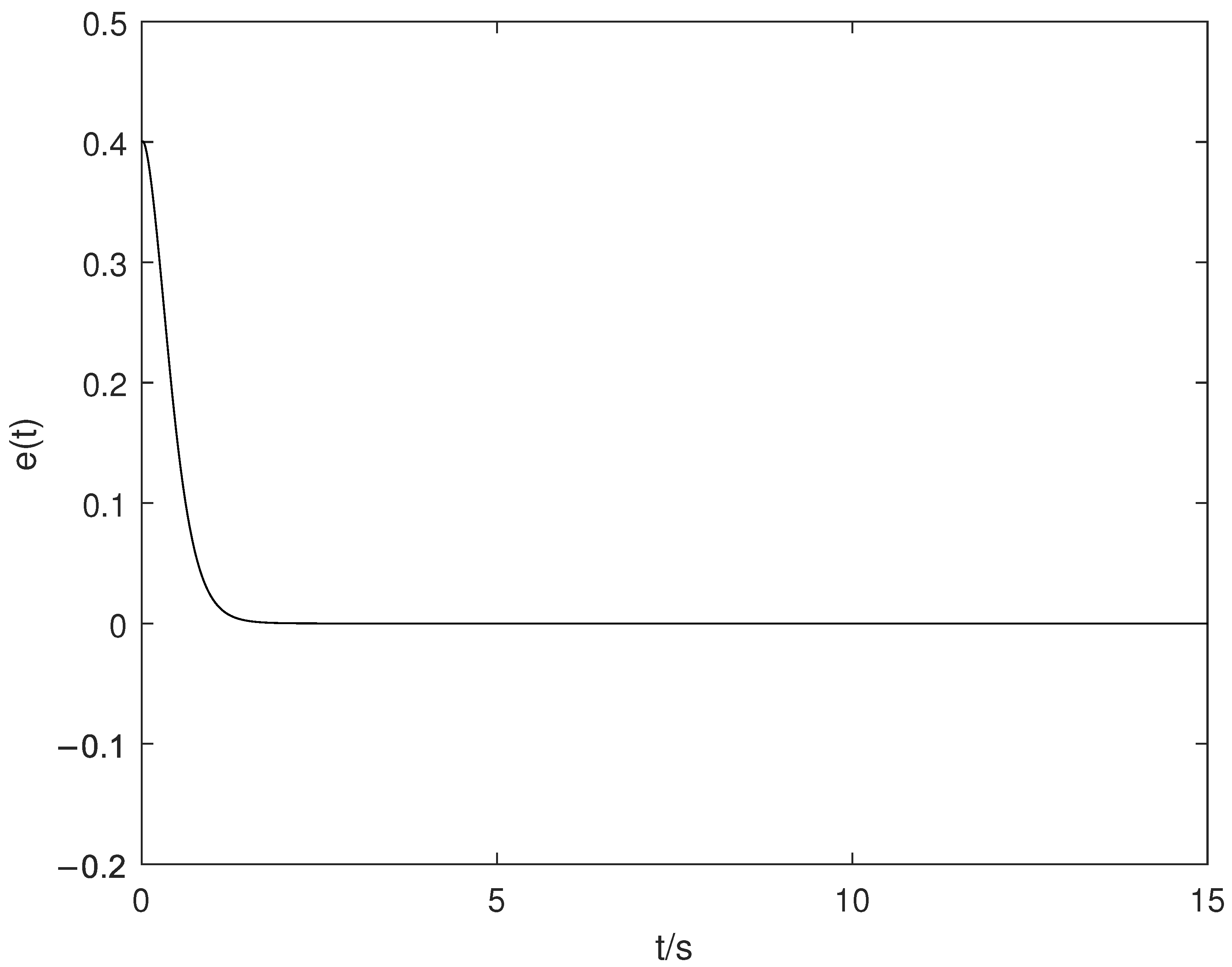
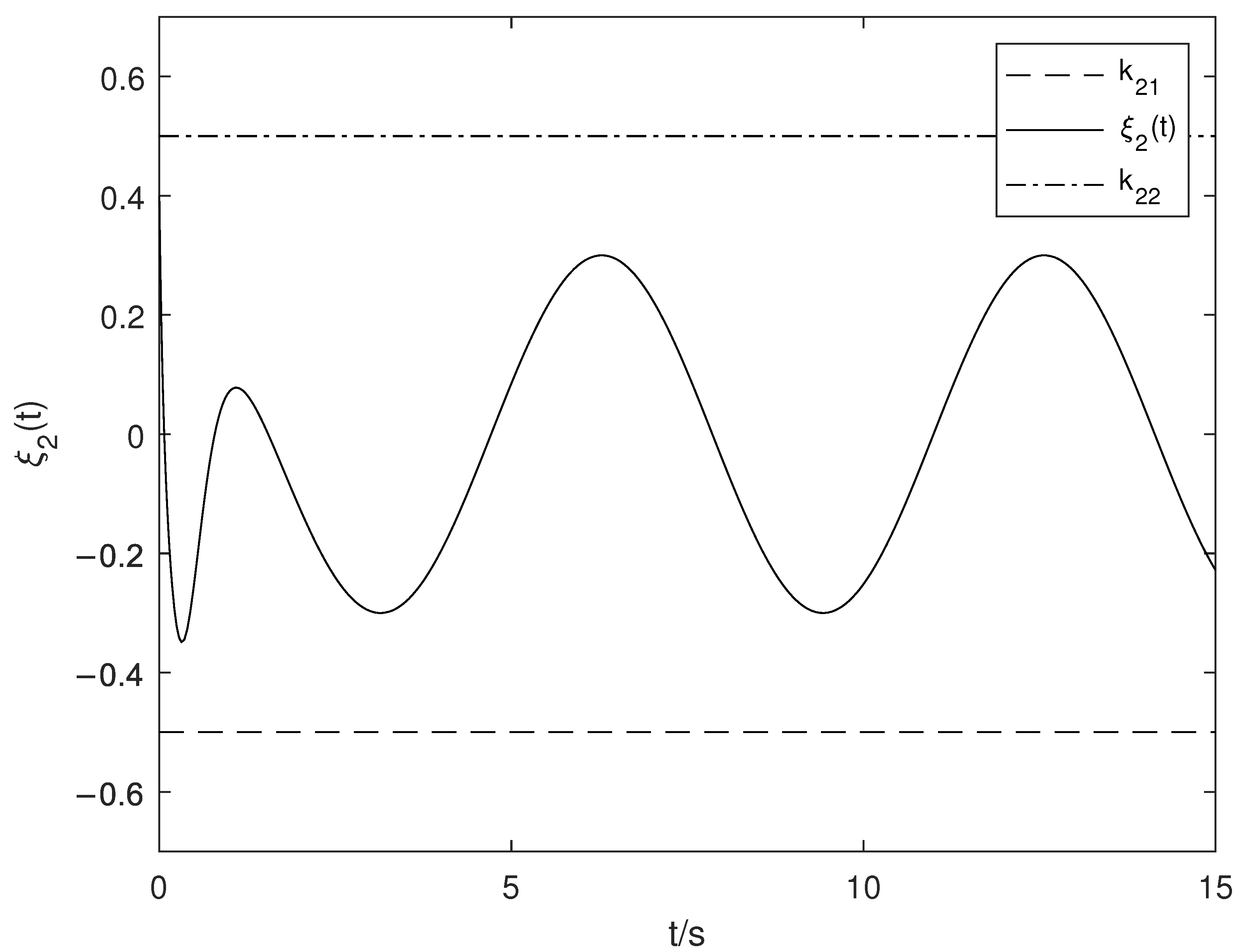
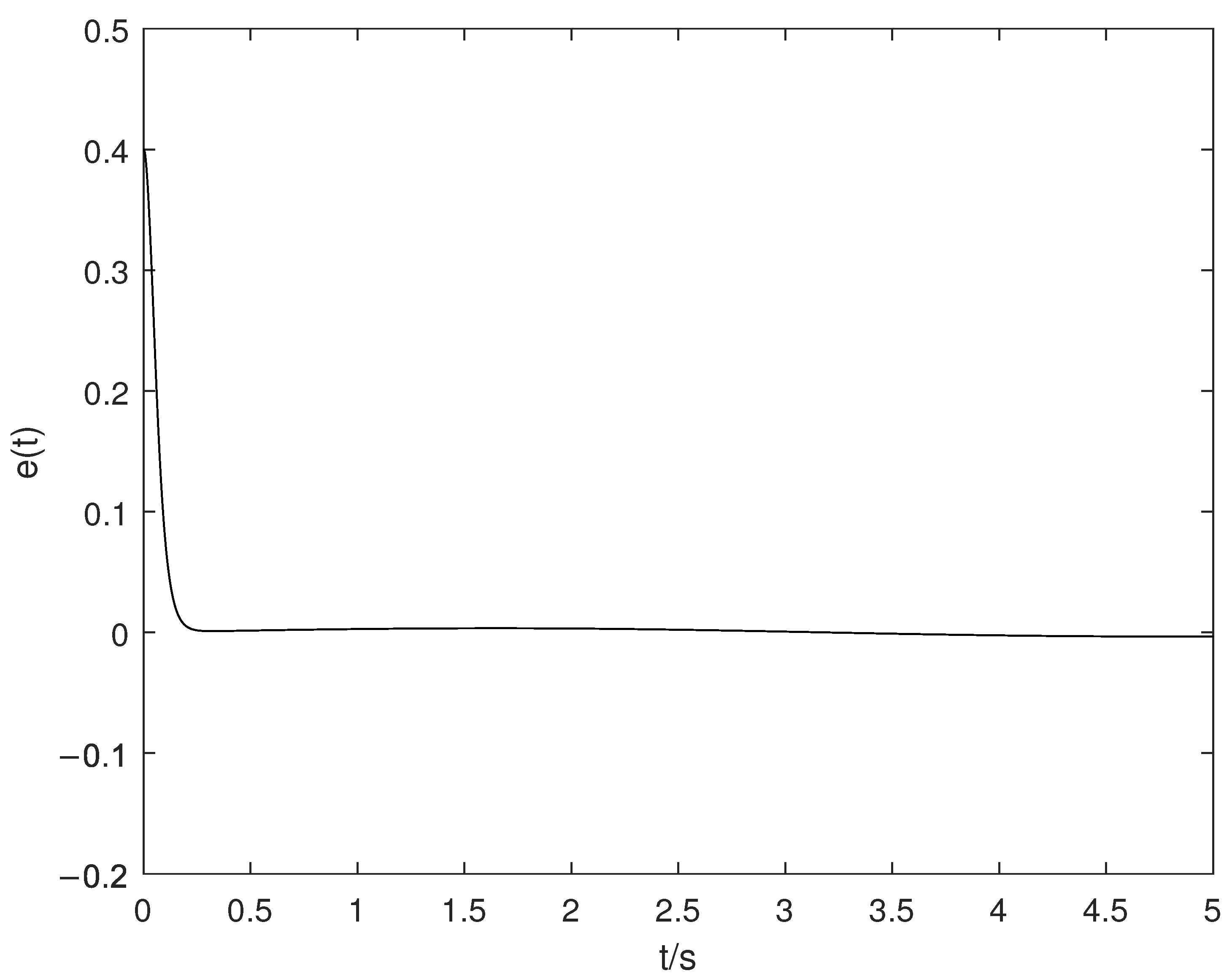
5. Simulation Example

Example 1.
To better reflect the effectiveness of the proposed algorithm, we use the mathematical model of the single-link robot to verify it in this section. According to [34,35], the mathematical model of a single-link robot is as follows:
M 0 q ¨ + 1 2 m g l sin ( q ) = u ,
where u is the input torque; q is the angle; M 0 is the moment of inertia; g is the acceleration caused by gravity; m and l are the mass and length of the connecting rod.
Define ξ 1 = q and ξ 2 = q ˙ . Then, system (1) is expressed as
ξ ˙ 1 ξ ˙ 2 = 0 1 0 0 ξ 1 ξ 2 + 0 1 [ u M 0 m g l sin ( ξ 1 ) 2 M 0 ] ,
where f 1 ( ξ 1 ) = 0 , and f 2 ( ξ ¯ 2 ) = m g l sin ( ξ 1 ) 2 M 0 . According to [10], m = 1 k g , l = 1 m , M 0 = 0.5 k g m 2 and g = 9.8 N / k g .
Define constraint functions as
x 1 = ln ξ 1 ( t ) k 11 k 12 ξ 1 ( t ) , x 2 = ln ξ 2 ( t ) k 21 k 22 ξ 2 ( t ) .
Then, we have
x ˙ 1 = F 1 ( x ¯ 1 , x 2 ) , x ˙ 2 = g 2 ( x 2 ) u + F 2 ( x ¯ 2 ) ,
where
F 1 ( x ¯ 2 ) = g 1 ( x 1 ) k 22 e x 2 + k 21 1 + e x 2 ,
g i ( x i ) = ( 1 + e x i ) 2 ( k i 2 k i 1 ) e x i , i = 1 , 2 ,
F 2 ( x ¯ 2 ) = g 2 ( x 2 ) f 2 ( k 12 e x 1 + k 11 1 + e x 1 , k 22 e x 2 + k 21 1 + e x 2 ) .
Define θ 1 = x 1 and θ 2 = θ ˙ 1 . According to (25), we have
θ ˙ 1 = θ 2 , θ ˙ 2 = a 2 ( x ¯ 2 ) + b 2 ( x ¯ 2 ) u .
Then, we use the backstepping method to redefine η 1 = θ 1 Y 0 and η 2 = θ 2 α 1 . The controller is designed as
α 1 = ε 1 η 1 + Y ˙ 0 , u = 1 b 2 ( x ¯ 2 ) [ ε 2 η 2 + α ˙ 1 a 2 ( x ¯ 2 ) ] .
In this paper, the constraints of system states are required to satisfy 0.5 < ξ 1 < 0.5 and 0.5 < ξ 2 < 0.5 , so we design the constraint parameters as k 11 = 0.5 , k 12 = 0.5 , k 21 = 0.5 and k 22 = 0.5 . The control gain can be assigned to ε 1 = 5 and ε 2 = 5 . At the same time, the initial values of system states are ξ 1 ( 0 ) = 0.4 and ξ 2 ( 0 ) = 0.4 .
After calculation, we have the following deduction according to the NOTC condition (47)
η 1 ( 0 ) = 2 ln ( 3 2 ) > 0 , η 2 ( 0 ) = 40 9 + 10 ln ( 3 2 ) 1.2 > 0 e ( t ) > 0 .
The simulation results are shown in Figure 1, Figure 2 and Figure 3.
Figure 1 shows the time trajectories of tracking error e ( t ) . Figure 2 shows the time trajectory of system state ξ 1 ( t ) . Figure 3 shows the time trajectory of system state ξ 2 ( t ) . Figure 4 shows the time trajectory of u ( t ) . According to Figure 1, Figure 2, Figure 3 and Figure 4, we draw the following conclusions:
(1)
Figure 1 shows that the tracking error e ( t ) is non-overshoot, which shows that the non-overshoot algorithm in this paper is effective.
(2)
Figure 2 and Figure 3 shows that the trajectories of system states ξ 1 ( t ) and ξ 2 ( t ) are both within the constraint range. This shows that the constraint algorithm in this paper is effective.
Figure 5 is a simulation result obtained using the algorithm in Reference [36]. Then, compared with Figure 5, it is obvious that the overshoot of Figure 1 is smaller and the convergence speed is faster. This shows that the algorithm in this paper is superior.
Next, let ξ ˙ 1 = ξ 2 + 0.2 sin ( ξ 1 ) , where 0.2 sin ( ξ 1 ) can be assumed as disturbance or modeling error. Then, we set the control gain parameters as ε 1 = 10 and ε 2 = 10 . The rest of the data remain unchanged. We can obtain the simulation result as shown in Figure 6.
Figure 6 shows the trajectory of tracking error e ( t ) in the presence of disturbance. Although there is disturbance, the overshoot of tracking error e ( t ) is still almost zero. So the algorithm in this paper is effective.

6. Conclusions

In this paper, the FSCs control and NOTC of a class of nonlinear systems have been studied. Through two coordinate transformations, the system is transformed into a system whose subsystems are linear from the order 1 to the order n 1 . Based on backstepping, by designing the controller, a suitable CLS can be obtained; thus, the expression of tracking error can be obtained, and then the conditions of NOTC can be analyzed. The algorithm in this paper can not only make all the signals of the closed-loop system bounded, but can also make the overshoot of the system zero for each condition with non-overshooting. According to the simulation section, the algorithm in this paper is effective. The algorithm in this paper obtains more conditions with non-overshooting. Therefore, compared with the existing results, the algorithm in this paper reduces the conservatism.
The method proposed in this paper primarily focuses on the research findings for SISO systems. Compared to such systems, MIMO systems are more aligned with practical requirements and represent a more generalized scenario. Therefore, future work will investigate the non-overshooting control problem for multi-input–multi-output systems.

Author Contributions

Conceptualization, X.-Q.X. and C.Z.; Methodology, X.-Q.X.; Formal analysis, C.Z.; Investigation, C.Z.; Resources, C.Z.; Data curation, X.-Q.X.; Writing—original draft, X.-Q.X. and C.Z.; Visualization, X.-Q.X.; Supervision, C.Z.; Project administration, C.Z. All authors have read and agreed to the published version of the manuscript.

Funding

This work is partly supported by the Key Education Teaching Management Project of Anhui Province (2023JXGL039) and the “101 Plan” Project of Anhui Province (2023YLYJH038).

Institutional Review Board Statement

Not applicable.

Informed Consent Statement

Not applicable.

Data Availability Statement

The raw data supporting the conclusions of this article will be made available by the authors on request.

Acknowledgments

During the preparation of this manuscript, the authors used the Deespseek for the purposes of grammar checking and correcting typos. The authors have reviewed and edited the output and take full responsibility for the content of this publication.

Conflicts of Interest

The authors declare no conflicts of interest.

Abbreviations

The following abbreviations are used in this manuscript:
NOTCNon-Overshooting Tracking Control
FSCsFull-State Constraints
CLSClosed-Loop System
BLFBarrier Lyapunov Function

References

  1. Campbell, D.K. Nonlinear Science. In Los Alamos Science; University of Minnesota: Minneapolis, MN, USA, 1987. [Google Scholar]
  2. Cui, G.Z.; Xu, S.Y.; Ma, Q.; Li, Y.M.; Zhang, Z.Q. Prescribed performance distributed consensus control for nonlinear multi-agent systems with unknown dead-zone input. Int. J. Control 2018, 91, 1053–1065. [Google Scholar] [CrossRef]
  3. Zhang, T.L.; Su, S.F.; Wei, W.; Yeh, R.H. Practically Predefined-Time Adaptive Fuzzy Tracking Control for Nonlinear Stochastic Systems. IEEE Trans. Cybern. 2023, 53, 8000–8012. [Google Scholar] [CrossRef]
  4. Zhao, K.; Song, Y.D.; Ma, T.D.; He, L. Prescribed Performance Control of Uncertain Euler-Lagrange Systems Subject to Full-State Constraints. IEEE Trans. Neural Netw. Learn. Syst. 2018, 29, 3478–3489. [Google Scholar] [PubMed]
  5. Shi, S.; Gu, J.; Xu, S.Y.; Min, H.F. Globally Fixed-Time High-Order Sliding Mode Control for New Sliding Mode Systems Subject to Mismatched Terms and Its Application. IEEE Trans. Ind. Electron. 2020, 67, 10776–10786. [Google Scholar] [CrossRef]
  6. Wang, L.; Sun, W.; Su, S.F.; Zhao, X.D. Adaptive Asymptotic Tracking Control for Flexible-Joint Robots With Prescribed Performance: Design and Experiments. IEEE Trans. Syst. Man Cybern. Syst. 2023, 53, 3707–3717. [Google Scholar] [CrossRef]
  7. Tang, F.H.; Niu, B.; Wang, H.Q.; Zhang, L.; Zhao, X.D. Adaptive Fuzzy Tracking Control of Switched MIMO Nonlinear Systems With Full State Constraints and Unknown Control Directions. IEEE Trans. Circ. Syst. II-Express Briefs 2022, 69, 2912–2916. [Google Scholar] [CrossRef]
  8. Tran, T.T. Feedback linearization and backstepping: An equivalence in control design of strict-feedback form. IMA J. Math. Control Inf. 2020, 37, 1049–1069. [Google Scholar] [CrossRef]
  9. Min, H.F.; Xu, S.Y.; Zhang, B.Y.; Ma, Q.; Yuan, D.M. Fixed-Time Lyapunov Criteria and State-Feedback Controller Design for Stochastic Nonlinear Systems. IEEE-CAA J. Autom. Sin. 2022, 9, 1005–1014. [Google Scholar] [CrossRef]
  10. Edwards, C.; Spurgeon, S.K. Sliding Mode Control: Theory and Applications; CRC Press: Boca Raton, FL, USA, 1998. [Google Scholar]
  11. Liu, S.L.; Niu, B.; Zong, G.D.; Zhao, X.D.; Xu, N. Adaptive Neural Dynamic-Memory Event-Triggered Control of High-Order Random Nonlinear Systems with Deferred Output Constraints. IEEE Trans. Autom. Sci. Eng. 2018, 21, 923–933. [Google Scholar] [CrossRef]
  12. Jia, F.J.; Lu, J.W.; Li, Y.M. Neural network adaptive output regulation for non-linear uncertain systems with full-state constraints. IMA J. Math. Control Inf. 2021, 38, 992–1009. [Google Scholar] [CrossRef]
  13. Liu, Y.J.; Tong, S.C. Barrier Lyapunov Functions-based adaptive control for a class of nonlinear pure-feedback systems with full state constraints. Automatica 2016, 64, 70–75. [Google Scholar] [CrossRef]
  14. Jia, F.J.; Yan, X.; Wang, X.H.; Lu, J.W.; Li, Y.M. Robust adaptive prescribed performance dynamic surface control for uncertain nonlinear pure-feedback systems. J. Frankl. Inst. 2020, 357, 2752–2772. [Google Scholar] [CrossRef]
  15. Liang, X.L.; Ge, S.S.; Li, D.Y. Coordinated tracking control of multi agent systems with full-state constraints. J. Frankl. Inst. 2023, 360, 12030–12054. [Google Scholar] [CrossRef]
  16. Niu, B.; Zhang, Y.; Zhao, X.D.; Wang, H.Q.; Sun, W. Adaptive Predefined-Time Bipartite Consensus Tracking Control of Constrained Nonlinear MASs: An Improved Nonlinear Mapping Function Method. IEEE Trans. Cybern. 2023, 53, 6017–6026. [Google Scholar] [CrossRef]
  17. Ortiz, D.C.; Chairez, I.; Poznyak, A. Sliding-Mode Control of Full-State Constraint Nonlinear Systems: A Barrier Lyapunov Function Approach. IEEE Trans. Syst. Man Cybern. Syst. 2022, 52, 6593–6606. [Google Scholar] [CrossRef]
  18. Zhang, T.P.; Xia, M.Z.; Yi, Y. Adaptive neural dynamic surface control of strict-feedback nonlinear systems with full state constraints and unmodeled dynamics. Automatica 2017, 81, 232–239. [Google Scholar] [CrossRef]
  19. Krstic, M.; Bement, M. Nonovershooting control of strict-feedback nonlinear systems. IEEE Trans. Autom. Control 2006, 51, 1938–1943. [Google Scholar] [CrossRef]
  20. Zhan, J.Z.; Liu, Y.L. The design of a sinter furnace hearting control system for quick temperature rise without overshooting. Ind. Instrum. Autom. 2006, 3, 64–65. [Google Scholar]
  21. Darbha, S.; Bhattacharyya, S.P. On the synthesis of controllers for a non-overshooting step response. IEEE Trans. Autom. Control 2003, 48, 797–799. [Google Scholar] [CrossRef]
  22. Bement, M.; Jayasuriysa, S. Construction of a set of non-overshooting tracking controllers. J. Dyn. Syst. Meas. Control 2004, 126, 558–567. [Google Scholar] [CrossRef]
  23. Bement, M.; Jayasuriysa, S. Use of state feedback to achieve a non-overshooting step response for a class of non-minimum phase systems. J. Dyn. Syst. Meas. Control 2004, 126, 657–660. [Google Scholar] [CrossRef]
  24. Lin, S.K.; Fang, C.J. Nonovershooting and monotone nondecreasing step responses of a third-order SISO linear system. IEEE Trans. Autom. Control 1997, 42, 1299–1303. [Google Scholar]
  25. Darbha, S. On the synthesis of controllers for continuous time LTI systems that achieve a non-negative impulse response. Automatica 2003, 39, 159–165. [Google Scholar] [CrossRef]
  26. Chen, X.P.; Xu, H.B. Non-overshooting control for a class of nonlinear systems. Control Decis. 2013, 28, 627–631. [Google Scholar]
  27. Zhu, C.; Zhao, C.C. Non-overshooting output tracking of feedback linearisable nonlinear systems. Int. J. Control 2013, 86, 821–832. [Google Scholar] [CrossRef]
  28. Jia, F.J. Non-overshooting control of nonlinear pure-feedback systems. Syst. Control Lett. 2025, 185, 105743. [Google Scholar] [CrossRef]
  29. Jia, F.J. Non-overshooting tracking control for nonlinear systems with prescribed finite-time. ISA Trans. 2024, 151, 174–182. [Google Scholar] [CrossRef] [PubMed]
  30. Jia, F.J.; Zhu, Q.X. Non-Overshooting Tracking Control for Nonlinear Pure-Feedback Systems. IEEE Trans. Syst. Man Cybern. Syst. 2025, 55, 1277–1285. [Google Scholar] [CrossRef]
  31. Hazem, Z.B.; Guler, N.; Altaif, A.H. A study of advanced mathematical modeling and adaptive control strategies for trajectory tracking in the Mitsubishi RV-2AJ 5-DOF Robotic Arm. Discov. Robot. 2025, 1, 2. [Google Scholar] [CrossRef]
  32. Li, W.Q.; Krstic, M. Mean-nonovershooting control of stochastic nonlinear systems. IEEE Trans. Autom. Control 2021, 66, 5756–5771. [Google Scholar] [CrossRef]
  33. Song, L.; Tong, S.C. Finite-time mean-nonovershooting control for stochastic nonlinear systems. Int. J. Syst. Sci. 2023, 54, 1047–1055. [Google Scholar] [CrossRef]
  34. Tee, K.P.; Ge, S.Z. Control of nonlinear systems with partial state constraints using a barrier Lyapunov function. In. J. Control 2011, 84, 2008–2023. [Google Scholar] [CrossRef]
  35. Liu, J.; Chen, Z.Q.; Liu, Z.X.; Zhang, X.H. Distributed robust consensus control for nonlinear multiagent systems by using output regulation approach. IMA J. Math. Control Inf. 2014, 32, 515–535. [Google Scholar] [CrossRef]
  36. Jia, F.J.; Lu, J.W.; Li, Y.M.; Li, F.Y. Fuzzy adaptive stabilization control for nonlinear systems with FSCs. Fuzzy Sets Syst. 2024, 473, 108738. [Google Scholar] [CrossRef]
Figure 1. The time trajectories of e ( t ) .
Applsci 15 05816 g001
Figure 2. The time trajectory of ξ 1 ( t ) .
Applsci 15 05816 g002
Figure 3. The time trajectory of ξ 2 ( t ) .
Applsci 15 05816 g003
Figure 4. The time trajectory of u ( t ) .
Applsci 15 05816 g004
Figure 5. The time trajectories of e ( t ) in [36].
Applsci 15 05816 g005
Figure 6. The time trajectories of e ( t ) .
Applsci 15 05816 g006
Disclaimer/Publisher’s Note: The statements, opinions and data contained in all publications are solely those of the individual author(s) and contributor(s) and not of MDPI and/or the editor(s). MDPI and/or the editor(s) disclaim responsibility for any injury to people or property resulting from any ideas, methods, instructions or products referred to in the content.

