Methodology for Feature Selection of Time Domain Vibration Signals for Assessing the Failure Severity Levels in Gearboxes

Abstract

Early failure detection in gear systems reduces unplanned downtime and associated maintenance costs in rotating machinery. Although numerous indicators can be extracted from vibration signals, selecting the most relevant ones remains challenging. This study proposes a methodology for selecting time-domain features to classify fault severity levels in spur gearboxes. Vibration signals are acquired using six accelerometers and processed to extract 64 statistical condition indicators (CIs). The most informative subset of CIs is identified and selected through a wrapper-based selection approach and artificial intelligence tools. The selected features are then evaluated based on the classification accuracy and the area under the curve (AUC) in receiver operating characteristic (ROC) achieved using Random Forest (RF) and K-nearest neighbours (K-NN) models, with performance exceeding 98%. Additionally, the effect of sensor position and inclination on signal quality and classification performance is analysed using factorial analysis of variance (ANOVA) and multiple comparison tests. The results confirm the robustness of the selected CIs and the minimal influence of sensor placement variability, supporting the practical applicability of the proposed approach in industrial settings. The methodology offers a structured framework for selecting condition indicators in vibration signals, experimentally validated using multiple sensors and fault severity levels, and it is both automated and straightforward to implement.

1. Introduction

Transmission systems, particularly gearboxes, constitute critical subsystems in rotating machinery owing to their capability to deliver high-efficiency power transfer under confined spatial constraints and their ability to sustain elevated mechanical loads. For this reason, condition-based monitoring (CBM) is essential for the early detection of failures, helping to prevent machine operation downtime and unplanned maintenance activities [1,2].

Among the signals used in failure diagnosis, vibration stands out for its ease of acquisition and sensitivity to changes in mechanical conditions. However, its analysis is complex, including stationary, non-stationary, and resonant components [3,4]. This complexity necessitates applying advanced signal processing techniques to extract useful information for system diagnostics.

The monitoring process is typically divided into three stages: data acquisition, feature extraction, and failure identification. Data are captured via sensors placed at various locations on the system, providing accurate and reliable signals [5,6]. Feature extraction is then performed by calculating condition indicators (CIs), which are statistical parameters that reflect the system’s health condition [7,8,9].

CIs can be obtained in different domains. In the time domain, as shown in [10], in the frequency domain by transforming the signal from the time domain using the fast Fourier transform (FFT) [11], or in the time-frequency domain via wavelet transform [4,12]. In the time domain, CIs can be classified as conventional—such as root mean square, mean, variance, kurtosis, and skewness—or non-conventional, including absolute mean value, waveform length, zero crossings, Wilson amplitude, and slope sign changes, among others [13].

Several studies have shown that an appropriate combination of CIs enhances the sensitivity of diagnostic systems. However, a poor combination may introduce redundancy or contradictions that degrade model performance [14]. Consequently, feature selection is a crucial step in optimising classification models.

Feature selection is critical in developing machine learning models, particularly when dealing with high-dimensional data. The wrapper method is a feature selection technique that evaluates different subsets of variables based on the performance of a machine learning model, often resulting in improved predictive accuracy. This contrasts with filter methods, which assess variables independently of the model [15]. A significant advantage of the wrapper approach lies in its ability to identify combinations of features that may be uninformative in isolation but, when combined, enhance the model’s performance [5,16,17]. In this study, the wrapper method uses the Random Forest (RF) algorithm to rank the importance of the condition indicators (CIs).

To validate the proposed methodology, resampling techniques such as bootstrap and repeated hold-out are used to assess the model’s stability and the variability of the results [18,19]. For classification, machine learning models such as RF and K-NN are used, both of which are widely applied in the literature for failure detection in gearboxes [14,20,21,22].

Although there are studies that use CIs and statistical models for failure diagnosis [10,16], as well as investigations into optimal sensor placement [23,24], no methodology has been reported that combines CIs ranking through a wrapper approach with the evaluation of the effect of sensor position and inclination on diagnostic accuracy.

In this context, the objectives of this study are as follows: (a) To propose a feature selection methodology that establishes a CIs ranking based on time-domain vibration signals from a spur gearbox. (b) To evaluate the performance of the selected CIs using Random forest and K-nearest neighbours classification models. (c) To determine whether the sensor’s position and inclination significantly influence feature extraction and the performance of the classification model.

In summary, the main contributions of this work are:

1.

The design of a structured methodology for selecting relevant time-domain condition indicators from vibration signals.

2.

The validation of this selection using two widely adopted classifiers in the literature (Random Forest and K-nearest neighbours)

3.

The experimental evaluation of the effect of sensor position and inclination on fault classification performance in gear systems.

These contributions aim to support condition-based monitoring strategies that are robust, interpretable, and applicable in real industrial environments.

2. Materials and Methods

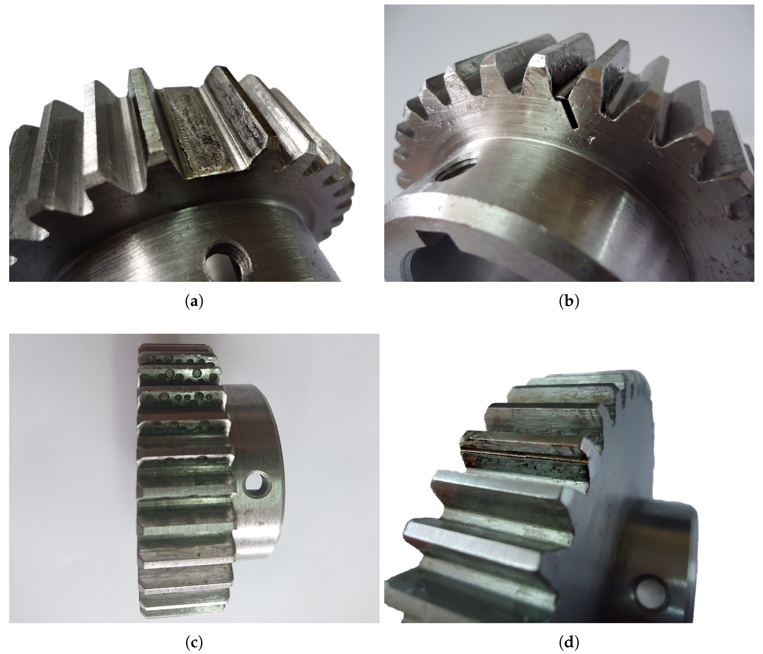
2.1. Experimental Bench

This work was developed with the vibration signal obtained from the experimental bench represented in Figure 1. It has a 1.5 kW, 1200 rpm, three-phase 220 V motor, and a 1.5 kW frequency inverter. The motor is coupled to a single-stage spur gearbox; the gears have Z1 = 32 and Z2 = 48 teeth. The load is simulated by an 8.83 kW electromagnetic brake on the output shaft. The vibration signal was obtained through six accelerometers (A1–A6) in (m/s²). Accelerometers A1, A4, A5, and A6 were installed in a vertical position defined by the z-axis. A1 and A4 were mounted on the gearbox’s input shaft, whereas A5 and A6 were installed on the output shaft to capture vibration signals associated with both transmission stages. Accelerometer A2 was mounted inclined ${45}^{\circ }$ concerning the x, and z axes, while A3 was mounted inclined ${45}^{\circ }$ concerning the x, y, and z axes. The vibration signal is fed to a computer, which collects the data using LabVIEW 2024 Q1 and Matlab R2024a software.

Four failure types were simulated on the gear Z1, breaking (Figure 2a), cracking (Figure 2b), pitting (Figure 2c), and scuffing (Figure 2d). Each failure mode was evaluated under baseline operating conditions (P1) and across nine progressive severity levels (P2–P10) to characterise the system’s response under varying failure intensities. Motor speed was adjusted to F1 = 8 Hz, F2 = 14 Hz, and F3 = 20 Hz using a frequency inverter, while load conditions were varied to L1 = 0 V, 10 V, and L3 = 20 V via an electromagnetic braking system. Considering ten severity levels, three motor speeds, three load conditions, and ten experimental repetitions, a database comprising 900 observations per accelerometer was generated.

The experimental bench also has an encoder (E1), a laser encoder (LE1), two acoustic emission sensors (EA), and two microphones (M) for the gearbox and the power supply lines to the motor with three voltage meters (V) and three electric current clamp (CC).

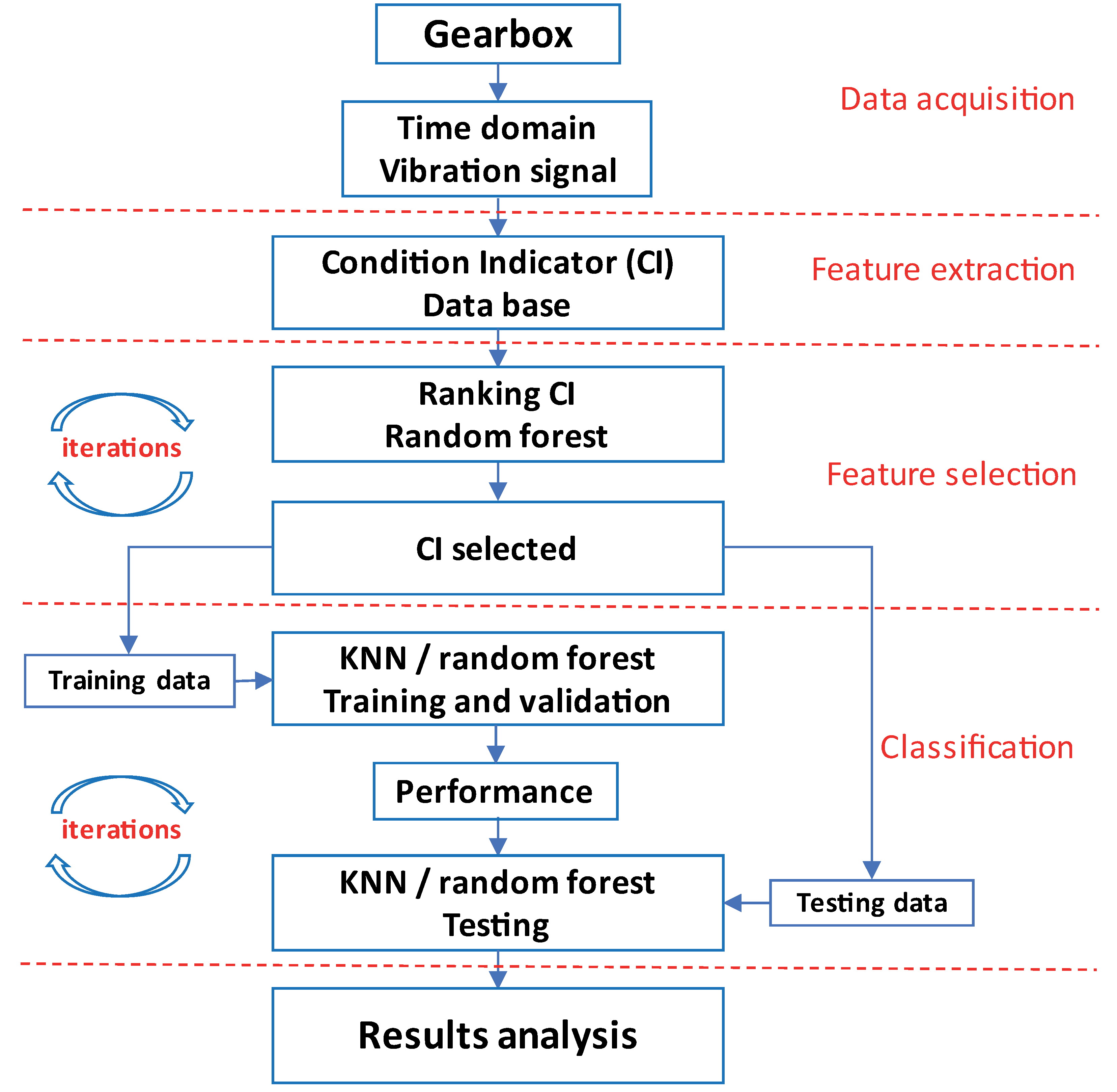
2.2. Methodology

The methodology proposed is outlined in Figure 3. It comprises the following stages: acquisition of vibration data, extraction and selection of features, classification of failure severity levels, and statistical evaluation of the effects of sensor positioning and inclination.

2.2.1. Data Acquisition

Using six accelerometers (A1–A6) installed at different positions and inclinations on the gearbox, the vibration signal (Figure 4) was obtained. Each accelerometer sampled data at a frequency of 50 kHz, and a 10 s acquisition period produced 500,000 acceleration measurements per sensor.

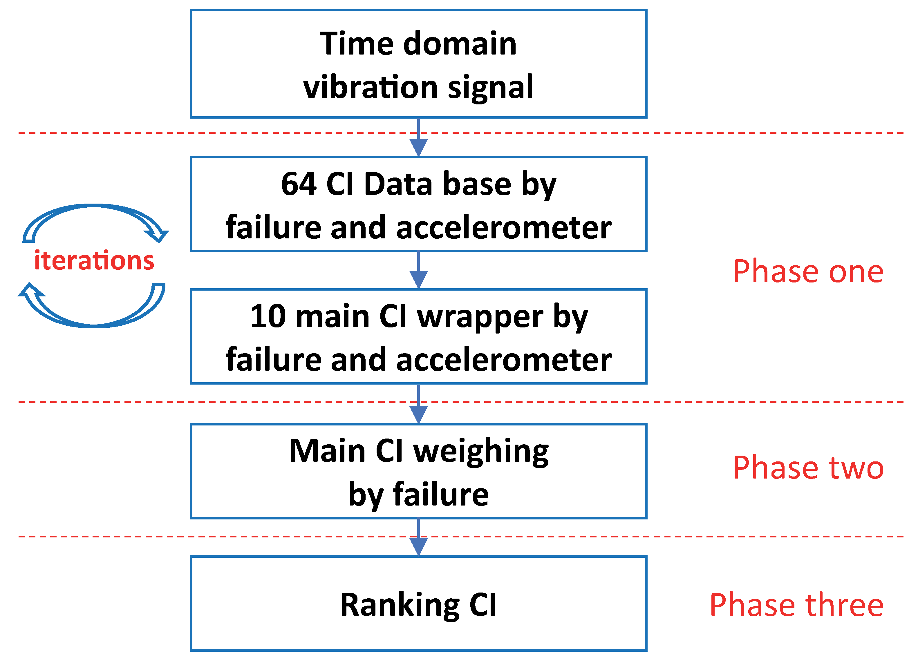
2.2.2. Feature Extraction

Feature extraction from the time-domain vibration signals was done using 64 condition indicators (CIs) for each accelerometer and failure type. These indicators effectively capture different aspects of vibration dynamics in mechanical systems [13]. The detailed formulas and descriptions of the studied CIs can be found in Appendix A.

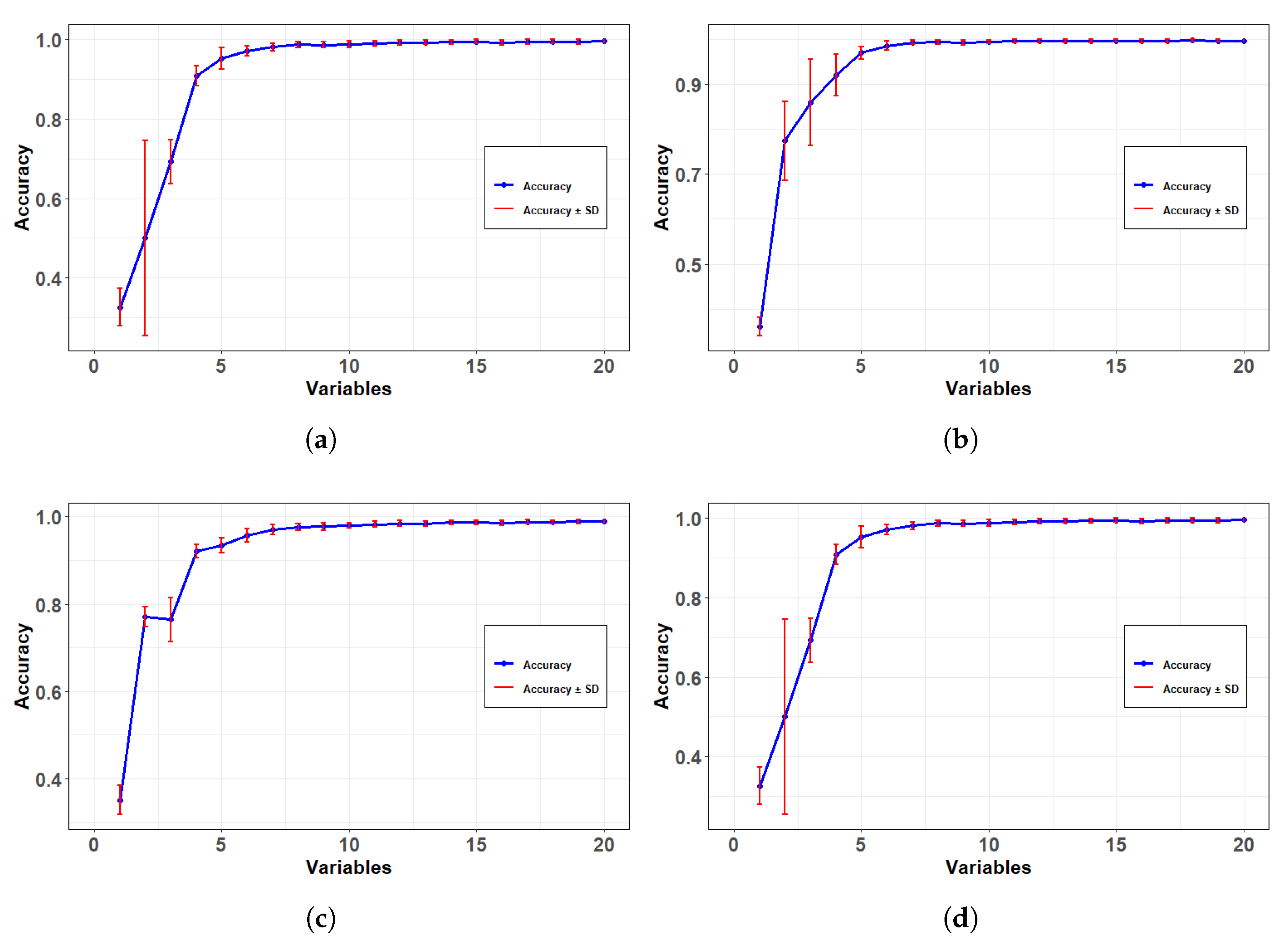
2.2.3. Feature Selection

Feature selection focused on the data acquired by accelerometers A1, A2, and A3, while the remaining accelerometers (A4, A5, and A6) were used to validate the robustness of the selected subset. The selection process is illustrated in Figure 5.

A wrapper-based approach was employed using the random forest (RF) classifier, as this type of method evaluates the performance of feature subsets within the learning model itself, improving selection quality. Additionally, RF allows for estimating each CI relative importance by calculating its mean influence (MI) on the model’s performance.

The selection process consisted of the following phases:

• Phase 1:

Preparation of the RF classification model (mathematically detailed in Section 2.2.4) was carried out by optimising its hyperparameters, using the 64 computed condition indicators (CIs). These CIs were iteratively introduced into the classification model, with the training dataset (from accelerometers A1–A3) being resampled using the bootstrap method until maximum accuracy was achieved.

The machine learning wrapper method was applied once the RF classifier’s hyperparameters were optimised. This consisted of testing and evaluating different combinations of CIs to determine which yielded the best performance within the RF model, based on the average importance of each CI. The top 10 most relevant CIs were selected for each accelerometer, and a descending weight from 10 to 1 was assigned according to their ranking.

• Phase 2:

The weights of each CI were summed by failure type across the three accelerometers to determine their relative influence of each kind of failure.

• Phase 3:

Finally, the weights accumulated for each failure type were aggregated. The CIs with the highest total weights that appeared across all failure types were selected. This resulted in a final subset of the 7 most relevant CIs used as input for classification models. The monitoring method is ready for implementation with the selected condition indicators and the optimised classification model.

2.2.4. Classification Models

In this study, the performance of the selected condition indicators (CIs) was evaluated using two classification models: Random Forest (RF) and K-nearest Neighbours (K-NN), both widely recognised and proven to be effective in fault diagnosis tasks [4,14,20,21,22]. RF was used as the primary model, and K-NN was applied as a comparative technique. These algorithms were selected due to their robustness, interpretability, simplicity, low computational demand, reduced sensitivity to noise, and ease of implementation—qualities that make them particularly suitable for real-time industrial applications [25,26,27]. Their use is therefore justified in scenarios where timely and reliable fault detection is prioritised over theoretical optimality [28,29].

Although more complex models, such as deep neural networks or advanced ensemble architectures, are available, they typically require larger datasets, greater computational capacity, and often lack interpretability. In contrast, RF and K-NN offer optimal performance with minimal parameter tuning and allow better traceability of each CI’s contribution to the classification outcome, which is essential for practical industrial monitoring applications.

Moreover, these classifiers enable a direct validation of the selected subset of CIs, supporting the analysis of their relationship with varying fault severity levels.

• Random forest (RF): RF is a classification model represented by Equation (1), composed of multiple tree-based classifiers. For each ith tree, an independent random vector $\left(V_i\right)$ is generated. Each tree is trained on a subset of the data and votes for the most popular category in the input vector $\left(x\right)$. The classification error, described by Equation (2), depends on the margin $\left(mg\right)$, which measures the average number of votes received for the correct class, and on the probability distribution $P_{X,Y}$ in the feature-label space [30].

  $$RF=h{(x,V_i)}_{i=1}^N,i=1,2,3...,N$$

  (1)

  $$E=P_{X,Y}\left(mg(X,Y)\right)$$

  (2)
• k-nearest neighbours (K-NN): K-NN is a non-parametric algorithm used for classification tasks in which new instances are categorised based on their proximity to existing samples within the feature space. The method assigns weights according to distance and infers the class of an unknown observation through a majority voting mechanism [31]. K-NN requires only the selection of the parameter k to define the number of neighbours and the appropriate distance metric [32].
  The K-NN classification algorithm works as follows:
  Given a training set $D{(x_i,y_i)}_{i=1}^N$, where $x_i$ is a training vector and $y_i$ its class label, and a test instance $(x^{\prime },y^{\prime })$, the predicted class $y^{\prime }$ is determined using Equation (3):

  $$y^{\prime }=\underbrace{\arg \max }\psi \sum (x^{\prime },y^{\prime })\in D^{\prime }{w}_i\delta (\psi ,y_i)$$

  (3)
  Here, $\psi$ is a candidate class label, $y_i$ is the label of the ith nearest neighbour, $\delta (·)$ is the indicator function returning 1 if the labels match and 0 otherwise, and $w_i$, as defined in Equation (4), represents a weighting coefficient derived from the distance $d(x^{\prime },x_i)$ between the query instance and its ith nearest neighbour.

  $$w_i={\displaystyle \frac{1}{{\left(d(x^{\prime },x_i)\right)}^2}}$$

  (4)
  The default distance metric is Euclidean, although alternatives such as Mahalanobis, Manhattan, and Minkowski distances can also be used [33].

A repeated hold-out resampling process was applied to evaluate model performance. During each iteration, the databases were partitioned in 70% for model training and 30% for model testing. The method enables the estimation of model variability across multiple subsets and yields robust performance metrics such as the accuracy rate and the area under the curve (AUC) associated with the receiver operating characteristic (ROC) analysis [19,34]. Two vectors of 1000 observations were obtained for each accelerometer, failure type, and classification model—one for accuracy and one for AUC.

2.2.5. Analysis of the Effect of Sensor Position and Inclination on the Vibration Signal

The accuracy vectors obtained in Section 2.2.4 were analysed to assess the effect of sensor placement on model performance. Factorial analysis of variance (ANOVA) and post-hoc Tukey testing were applied to determine if sensor position and inclination, failure type, and classification model statistically impacted the results.

2.2.6. Computational Tools

All calculations, modelling, and statistical analyses were conducted using the R programming language within the RStudio 2024.04.0 integrated development environment [35]. Dedicated libraries were used for signal processing, statistical modelling, feature selection, and variance analysis.

3. Results and Discussion

The first objective of this work was to rank the CIs of the vibration signal in the time domain using the proposed methodology. In order to fulfil this objective, the process detailed in Section 2.2.3 was carried out.

By developing the procedure detailed in phase 1, the $\lambda$-value mtry = 11 was determined for the RF classifier. The top 10 CIs were selected because the variability in classification accuracy reduced for the four types of failures, as detailed in Figure 6. Subsequently, after assigning the weighting,

Table 1. Main CIs by failure and accelerometer.

Failure	A1		A2		A3		Weighing
	Variable (CI)	MI	Variable (CI)	MI	Variable (CI)	MI	Value
Breaking	TMHO	11.88	Mean	10.75	Zero crossing	11.74	10
	Mean	11.83	TMHO	10.70	Energy operator	11.18	9
	Zero crossing	11.17	Zero crossing	10.53	Mean	11.06	8
	Shape factor	9.78	Energy operator	10.48	TMHO	11.01	7
	SDIF	9.67	Kurtosis	9.31	SSC	10.94	6
	SSC	8.80	Latitud factor	9.11	Crest factor	9.14	5
	Skewness	8.73	Waveform	8.63	Impulse factor	8.93	4
	Energy operator	8.51	SSC	8.61	Latitud factor	8.89	3
	Margin index	8.43	Log-Log ratio	8.61	Kurtosis	8.32	2
	Log-Log ratio	8.28	Crest factor	8.59	Skewness	8.17	1
Crack	Skewness	11.29	SSC	10.14	Skewness	12.55	10
	Mean	10.06	Clearance factor	10.10	SSC	11.62	9
	TMHO	10.05	Skewness	9.88	Zero crossing	11.25	8
	Energy operator	9.98	TMHO	8.98	Energy operator	9.20	7
	SSC	9.38	Mean	8.95	FSM	9.14	6
	SDIF	9.03	FSM	8.93	Mean	8.82	5
	Kurtosis	8.95	Zero crossing	8.71	TMHO	8.81	4
	Shape factor	8.93	Kurtosis	8.32	Latitud factor	7.76	3
	FSM	8.89	NNNL	8.30	Clearance factor	7.32	2
	Zero crossing	8.55	Energy operator	7.84	Kurtosis	7.24	1
Pitting	Skewness	12.58	Energy operator	10.06	SSC	12.49	10
	TMHO	11.37	SSC	9.99	Mean	10.73	9
	Mean	11.25	TMHO	9.60	TMHO	10.70	8
	SDIF	10.09	Mean	9.55	Zero crossing	10.09	7
	Shape factor	10.06	Clearance factor	9.51	Energy operator	9.79	6
	FSM	9.03	Kurtosis	9.48	Skewness	9.39	5
	Kurtosis	8.80	Waveform	8.35	Kurtosis	8.37	4
	Energy operator	8.23	Shape factor	8.25	Latitud factor	8.17	3
	Latitud factor	8.23	Impulse factor	8.20	Shape factor	7.79	2
	Log-Log ratio	8.20	SDIF	8.15	SDIF	7.76	1
Scuffing	TMHO	11.82	TMHO	11.60	TMHO	11.69	10
	Mean	11.72	Mean	11.55	Mean	11.69	9
	Zero crossing	11.30	FSM	10.46	Skewness	10.92	8
	Skewness	10.47	Zero crossing	9.95	FSM	10.67	7
	SDIF	10.11	Skewness	8.69	Energy operator	8.54	6
	Shape factor	9.80	Waveform	8.65	Impulse factor	8.18	5
	SSC	9.60	Clearance factor	8.51	Zero crossing	8.02	4
	Kurtosis	9.04	Pulse	8.42	Kurtosis	8.01	3
	FSM	8.38	Kurtosis	8.26	Clearance factor	7.99	2
	Wavelength	8.34	Impulse factor	8.23	Crest factor	7.94	1

TMHO = Temporal moments higher order; SDIF = Standard deviation impulse factor; SSC = Slope sign change; FSM = Fifth statistic moment; NNNL = Normalized normal negative likelihoog.

was obtained for breaking (B), cracking (C), pitting (P), and scuffing (S) failures.

In order to determine the CIs weighting by failure types, phase 2 was carried out, and the results presented in

Table 2. Main CIs for failure.

CI Breaking	Weighing	CI Cracking	Weighing	CI Pitting	Weighing	CI Scuffing	Weighing
Mean	27	Skewness	28	TMHO	25	TMHO	30
Zero crossing	26	SSC	25	Mean	24	Mean	27
TMHO	26	Mean	20	Energy operator	19	Skewness	21
Energy operator	19	TMHO	19	SSC	19	Zero crossing	19
SSC	14	Energy operator	15	Skewness	15	FSM	17
Kurtosis	8	FSM	13	Kurtosis	13	Kurtosis	8
Latitud factor	8	Zero crossing	13	Shape factor	11	Energy operator	6
Shape factor	7	Clearance factor	11	SDIF	9	Impulse factor	6
SDIF	6	Kurtosis	8	Zero crossing	7	Clearance factor	6
Crest factor	6	SDIF	5	Clearance factor	6	SDIF	6
Skewness	5	Shape factor	3	FSM	5	Shape factor	5
Waveform	4	Latitud factor	3	Latitud factor	5	Waveform	5
Impulse factor	4	NNNL	2	Waveform	4	SSC	4
Log-Log ratio	3			Impulse factor	2	Pulse index	3
Margin index	2			Log-Log ratio	1	Wavelength	1
						Crest factor	1

were obtained.

The total weighting and count per failure types in the CIs exposed in phase 3 are detailed in

Table 3. Ranking CI.

Ranking CI	# Failures	Weighing	Ranking CI	# Failures	Weighing
TMHO	4	100	Clearance factor	3	23
Mean	4	98	Latitud factor	3	16
Skewness	4	70	Waveform	3	13
Zero crossing	4	65	Impulse factor	3	12
SSC	4	61	Crest factor	2	7
Energy operator	4	59	Log-Log ratio	2	5
Kurtosis	4	37	Pulse	1	3
FSM	3	35	Verosneg	1	2
SDIF	4	27	MarginI	1	1
Shape factor	4	25	Wavelength	1	1

. The top 7 CIs were selected because they have the highest weighting and are present in all failure types. This procedure reduces the dimensionality of the DBs.

The CIs selected in the ranking were Temporal moments higher order (TMHO), Mean, Skewness, Zero crossing, Slope sign change (SSC), Energy operator and Kurtosis. The calculation equations of the CIs are detailed in

Table 4. Main CIs formulas.

CI	Formula
Temporal moments higher order	$|{\displaystyle \frac{1}{N}}{\sum }_{i=1}^N{x}_i^m|$ m = 3 as default
Mean	${\displaystyle \frac{1}{N}}{\sum }_{i=1}^N{x}_i$
Skewness	${\displaystyle \frac{N{\sum }_{i=1}^N{(x_i-T1)}^3}{T{3}^3}}$
Zero crossing	$$\begin{gathered} {\sum }_{i=1}^{N}step\left[sign(-x_i\ast x_{i+1})\right] \\ step=\left\{\begin{array}{c}1,ifx>0\\ 0,ifx=0\\ -1,ifx<0\end{array}\right. \\ sign=\left\{\begin{array}{c}1,ifx>0\\ {\displaystyle \frac{1}{2}},ifx=0& \\ 0,ifx<0\end{array}\right. \end{gathered}$$
Slope sign change	$$\begin{gathered} {\sum }_{i=2}^{N}f[(x_i-x_{i-1})\ast (x_i-x_{i+1})] \\ f=\left\{\begin{array}{c}1,ifx\ge threshold\\ 0,otherwise\end{array}\right. \end{gathered}$$
Energy operator	${\displaystyle \frac{N^2{\sum }_{i=1}^N{(\Delta y_i-\Delta \overline{y})}^4}{{\left[{\sum }_{i=1}^N{(\Delta y_i-\Delta \overline{y})}^2\right]}^2}}$
Kurtosis	${\displaystyle \frac{N{\sum }_{i=1}^N{(x_i-T1)}^4}{{\left[{\sum }_{i=1}^N{(x_i-T1)}^2\right]}^2}}$

. With the selected CIs, new DBs with 900 observations and these 7 CIs were constructed. These DBs were used to compute the accuracy and AUC metrics for the RF and k-nn algorithms.

A complementary statistical analysis was incorporated based on the Bhattacharyya distance [36] to strengthen the validity of the final set of selected features, quantifying the separation of condition indicators (CIs) across class distributions. This metric was calculated for all 64 CIs, considering comparisons between the baseline class (P1) and the various fault severity levels.

The results showed that the CIs selected through the proposed wrapper-based approach exhibited higher Bhattacharyya distance, confirming their discriminative capability. In contrast, multiple CIs with consistently low distances were identified and not selected during the feature selection phase, reinforcing the consistency between the statistical analysis and the multivariable classification performance. This comparison is detailed in

Table 5. Bhattacharyya distance by CIs in breaking failure.

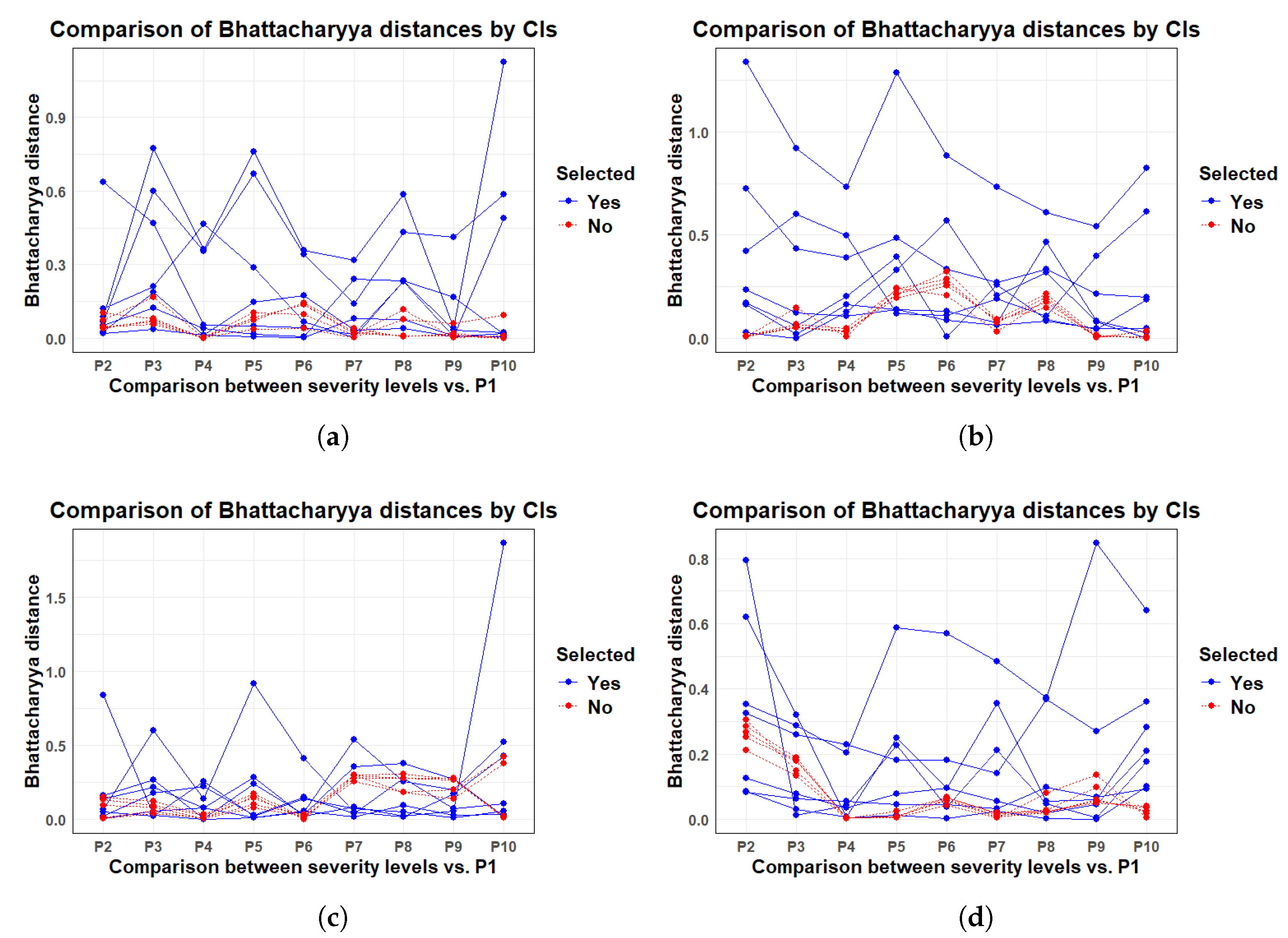
CI	P10_P1	P2_P1	P3_P1	P4_P1	P5_P1	P6_P1	P7_P1	P8_P1	P9_P1	Selected
Mean	0.0064	0.0201	0.0358	0.0120	0.0078	0.0022	0.0814	0.0765	0.0093	✓
Kurtosis	1.1276	0.0884	0.7727	0.3634	0.7616	0.3588	0.3181	0.5865	0.0418	✓
Skewness	0.5866	0.0673	0.5990	0.3561	0.6712	0.3422	0.1406	0.4332	0.4136	✓
Energy operator	0.4896	0.6353	0.4698	0.0545	0.0502	0.0424	0.0176	0.2303	0.0057	✓
Zero crossing	0.0179	0.1221	0.2126	0.4674	0.2867	0.0666	0.0040	0.2359	0.1662	✓
Slope sign change	0.0194	0.0261	0.1891	0.0148	0.1490	0.1738	0.0322	0.0399	0.0064	✓
TMHO	0.0230	0.0533	0.1255	0.0410	0.0162	0.0074	0.2399	0.2359	0.0340	✓
Log detector	0.0006	0.0404	0.0724	0.0021	0.0840	0.1366	0.0213	0.0087	0.0112	X
Norm entropy	0.0007	0.0453	0.0661	0.0012	0.0823	0.1366	0.0281	0.0086	0.0149	X
Log energy entropy	0.0008	0.0476	0.0577	0.0019	0.0742	0.1435	0.0386	0.0073	0.0185	X
Wilson amplitude	0.0091	0.1034	0.0797	0.0033	0.1043	0.0973	0.0146	0.1169	0.0027	X
Mean square error	0.0950	0.0739	0.1665	0.0016	0.0375	0.0415	0.0025	0.0768	0.0597	X

,

Table 6. Bhattacharyya distance by CIs in cracking failure.

CI	P10_P1	P2_P1	P3_P1	P4_P1	P5_P1	P6_P1	P7_P1	P8_P1	P9_P1	Selected
Mean	0.0467	0.2361	0.1220	0.1081	0.1406	0.0883	0.0663	0.0858	0.0475	✓
Kurtosis	0.6123	0.4206	0.6007	0.4965	0.1207	0.1125	0.1914	0.1097	0.3974	✓
Skewness	0.1861	0.1702	0.0594	0.2048	0.3946	0.0068	0.2588	0.0923	0.0442	✓
Energy operator	0.8258	1.3385	0.9205	0.7314	1.2859	0.8833	0.7326	0.6106	0.5430	✓
Zero crossing	0.0289	0.1653	0.0218	0.1630	0.1393	0.1320	0.0774	0.4657	0.0853	✓
Slope sign change	0.0016	0.0301	0.0016	0.1294	0.3304	0.5692	0.2089	0.3196	0.0809	✓
TMHO	0.1989	0.7253	0.4340	0.3886	0.4875	0.3356	0.2727	0.3328	0.2164	✓
Log energy entropy	0.0069	0.0121	0.0523	0.0367	0.1946	0.2538	0.0917	0.1494	0.0118	X
Norm entropy	0.0074	0.0137	0.0577	0.0370	0.2174	0.2710	0.0837	0.1746	0.0093	X
Wave form	0.0370	0.0103	0.1494	0.0105	0.2426	0.2064	0.0313	0.1865	0.0043	X
Log detector	0.0093	0.0144	0.0666	0.0468	0.2375	0.2878	0.0763	0.2004	0.0075	X
Wilson amplitude	0.0018	0.0075	0.0526	0.0345	0.2109	0.3241	0.0926	0.2138	0.0181	X

,

Table 7. Bhattacharyya distance by CIs in pitting failure.

CI	P10_P1	P2_P1	P3_P1	P4_P1	P5_P1	P6_P1	P7_P1	P8_P1	P9_P1	Selected
Mean	0.0344	0.0079	0.0576	0.0756	0.0103	0.0551	0.0165	0.0969	0.0273	✓
Kurtosis	1.8664	0.1378	0.2153	0.0763	0.2812	0.0229	0.0822	0.0239	0.0544	✓
Skewness	0.4265	0.0650	0.6016	0.1370	0.9159	0.4084	0.0473	0.0161	0.1699	✓
Energy operator	0.5188	0.8403	0.0285	0.0011	0.0130	0.0513	0.5376	0.2571	0.2024	✓
Zero crossing	0.0545	0.0504	0.0194	0.2574	0.0243	0.1362	0.0741	0.0494	0.0109	✓
Slope sign change	0.0179	0.1600	0.2648	0.0039	0.2379	0.0339	0.3576	0.3789	0.2742	✓
TMHO	0.1061	0.0216	0.1777	0.2243	0.0270	0.1476	0.0393	0.2778	0.0729	✓
Clearence factor	0.3758	0.0045	0.0405	0.0121	0.1001	0.0329	0.2984	0.1857	0.1385	X
Pulse	0.4189	0.0105	0.0527	0.0051	0.0752	0.0239	0.2541	0.1810	0.1995	X
Wilson amplitude	0.0223	0.0961	0.0833	0.0059	0.1526	0.0015	0.3008	0.3050	0.2722	X
Log detector	0.0143	0.1348	0.0958	0.0278	0.1441	0.0088	0.2943	0.2784	0.2781	X
Norm entropy	0.0102	0.1506	0.1200	0.0335	0.1722	0.0168	0.2747	0.2784	0.2680	X

and

Table 8. Bhattacharyya distance by CIs in scuffing failure.

CI	P10_P1	P2_P1	P3_P1	P4_P1	P5_P1	P6_P1	P7_P1	P8_P1	P9_P1	Selected
Mean	0.0916	0.0829	0.0618	0.0545	0.0442	0.0441	0.0333	0.0979	0.0664	✓
Kurtosis	0.6395	0.3533	0.2871	0.2039	0.5874	0.5694	0.4844	0.3728	0.8484	✓
Skewness	0.2082	0.0850	0.0304	0.0070	0.2501	0.0966	0.0539	0.0202	0.0445	✓
Energy operator	0.1757	0.7935	0.0116	0.0435	0.2258	0.0384	0.2111	0.0480	0.0040	✓
Zero crossing	0.2809	0.1266	0.0771	0.0356	0.0772	0.0958	0.3544	0.0552	0.0606	✓
Slope sign change	0.0997	0.6204	0.3210	0.0049	0.0124	0.0011	0.0246	0.0010	0.0000	✓
TMHO	0.3601	0.3251	0.2599	0.2294	0.1819	0.1822	0.1395	0.3670	0.2683	✓
Wave form	0.0176	0.2126	0.1325	0.0012	0.0259	0.0645	0.0202	0.0260	0.0968	X
Log entropy	0.0391	0.2530	0.1784	0.0045	0.0060	0.0688	0.0162	0.0248	0.0505	X
Norm entropy	0.0336	0.2667	0.1801	0.0043	0.0066	0.0609	0.0128	0.0221	0.0559	X
Log Detector	0.0245	0.2847	0.1892	0.0042	0.0058	0.0564	0.0075	0.0193	0.0595	X
Wilson amplitude	0.0043	0.3042	0.1484	0.0051	0.0039	0.0429	0.0055	0.0799	0.1350	X

and visually represented in Figure 7.

Additionally, the methodological risk, widely discussed by Rencher [37], that some features with low individual informativeness could still provide value when combined with others, was taken into account. This risk was mitigated by employing a multivariable wrapper approach using Random Forest, which evaluates the performance of entire subsets of features and captures non-linear interactions.

In the work done by Nayana et al. [13], the vibration signal was analysed using 6 conventional and 6 non-conventional CIs to analyse bearing failures. In Sánchez et al. [10], feature extraction was performed starting from 30 CIs, and then a ranking of 10 CIs was performed using different filtering methods for different gear DB. In Patel et al. [38], 15 CIs were used to detect bearing failures. In contrast to the above mentioned works, we propose extracting features from the vibration signal using 64 CIs in the time domain. This leads to expand the options of CIs that can be included in the feature selection process for later use in the classification models.

The second objective presented was to measure the performance of the 7 selected CIs in the RF and K-NN classification models, for which, in the first instance, the $\lambda$-values in the classification models were determined and adjusted, being mtry = 3 for RF and k = 5 for K-NN. Subsequently, the accuracy and AUC in classifying the fault severity level were calculated. The results of the accuracy and AUC by accelerometer, failure and classifier are detailed in

Table 9. Accuracy by accelerometer, failure and classifier.

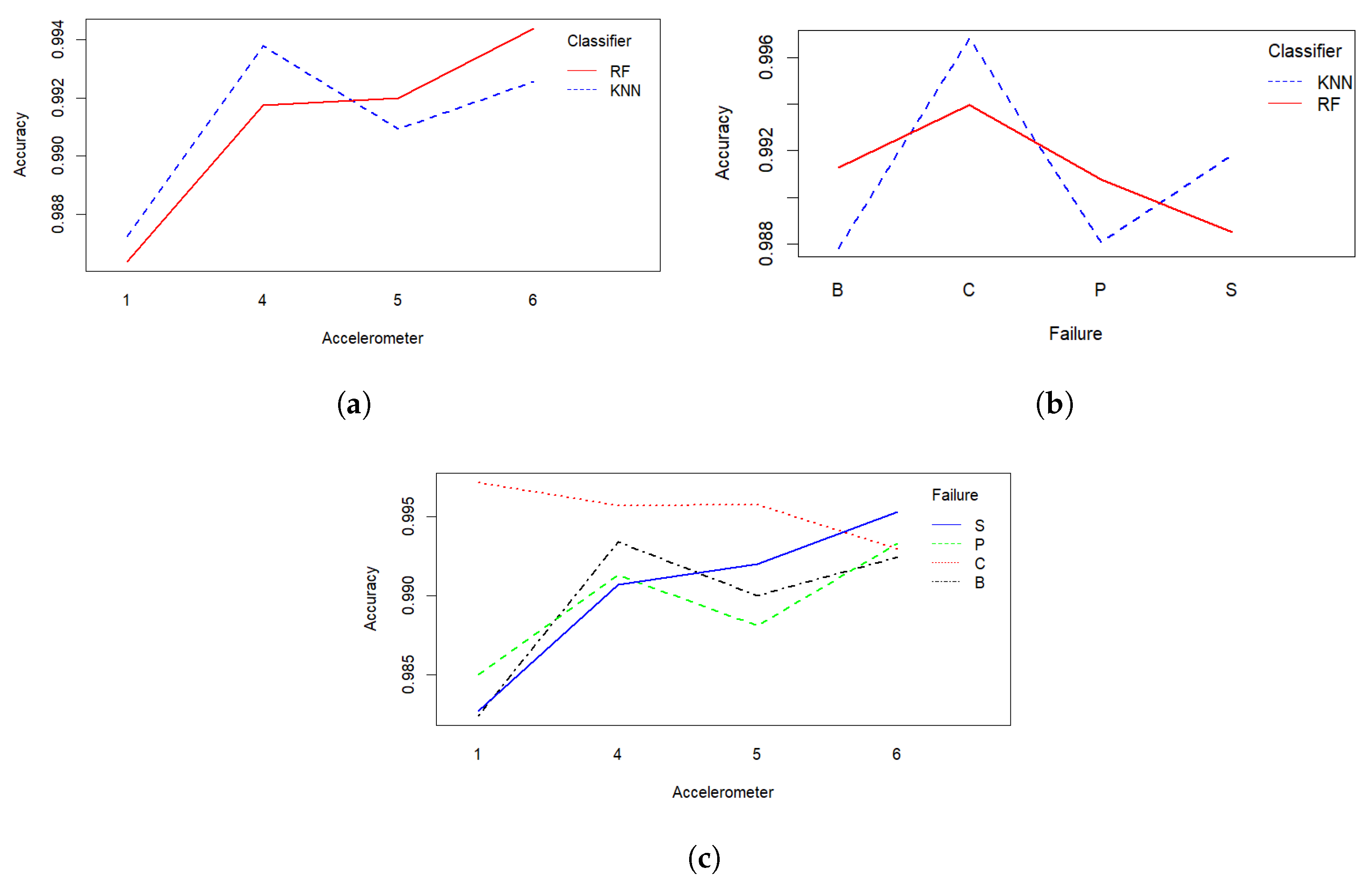
A	Breaking		Cracking		Pitting		Scuffing
	RF	K-NN	RF	K-NN	RF	K-NN	RF	K-NN
A1	0.9841	0.9807	0.9960	0.9983	0.9849	0.9850	0.9805	0.9850
A2	0.9884	0.9886	0.9948	0.9967	0.9921	0.9904	0.9827	0.9928
A3	0.9872	0.9826	0.9949	0.9909	0.9906	0.9928	0.9908	0.9959
A4	0.9908	0.9960	0.9939	0.9974	0.9923	0.9897	0.9894	0.9920
A5	0.9929	0.9871	0.9948	0.9967	0.9904	0.9858	0.9899	0.9941
A6	0.9974	0.9875	0.9911	0.9947	0.9947	0.9918	0.9943	0.9962

and

Table 10. AUC multiclass by accelerometer, failure and classifier.

A	Breaking		Cracking		Pitting		Scuffing
	RF	K-NN	RF	K-NN	RF	K-NN	RF	K-NN
A1	0.9922	0.9871	0.9965	0.9988	0.9885	0.9894	0.9905	0.9929
A2	0.9920	0.9930	0.9970	0.9982	0.9969	0.9962	0.9943	0.9968
A3	0.9956	0.9913	0.9950	0.9921	0.9935	0.9949	0.9952	0.9982
A4	0.9959	0.9980	0.9950	0.9987	0.9981	0.9967	0.9971	0.9970
A5	0.9964	0.9959	0.9983	0.9969	0.9926	0.9926	0.9961	0.9976
A6	0.9994	0.9960	0.9937	0.9961	0.9973	0.9978	0.9992	0.9990

respectively.

In Sánchez et al. [10], a 10 CIs ranking was performed using the filtering method for different gear DB in the time domain. When using the 10 CIs ranking in the RF and K-NN ranking models, the calculated accuracy in some DB was less than 85%. In the work done by Patel et al. [38], 15 CIs were used to detect bearing failures, resulting in values higher than 95% accuracy for the RF classification model. In this research, by using the wrapper method for the ranking of CIs and the RF and K-NN classification models, the classification accuracy and AUC values exceed 98%, as detailed in Table 9 and Table 10, respectively, when using only 7 CIs for all failure types, accelerometers and in the two classification models, thus reducing the dimensionality of the DB and increasing the efficiency in the classification process and reduce the computing time involved in processing the information.

The third objective of this work was to determine whether sensor position and inclination influence the extraction of vibration signal features for a classification model. To meet this objective, factorial ANOVA and Tukey’s post-hoc comparisons were conducted to assess differences in classification accuracy. The factors considered in the analysis were accelerometer position, failure, and the classification model employed.

The accelerometers A1, A4, A5 and A6 results were analysed to determine the influence of the sensor position. The ANOVA results indicated statistically significant differences (p-value < 0.001) in the average classification accuracy across the four accelerometers and for the four types of failure. In contrast, no significant difference was observed between the classification models (p-value = 1), while a significant interaction (p-value < 0.001) was found between the accelerometer:classifier (Figure 8a), failure:classifier (Figure 8b), and accelerometer:failure (Figure 8c) factors. A summary of the ANOVA results is presented in

Table 11. Anova factorial test for position.

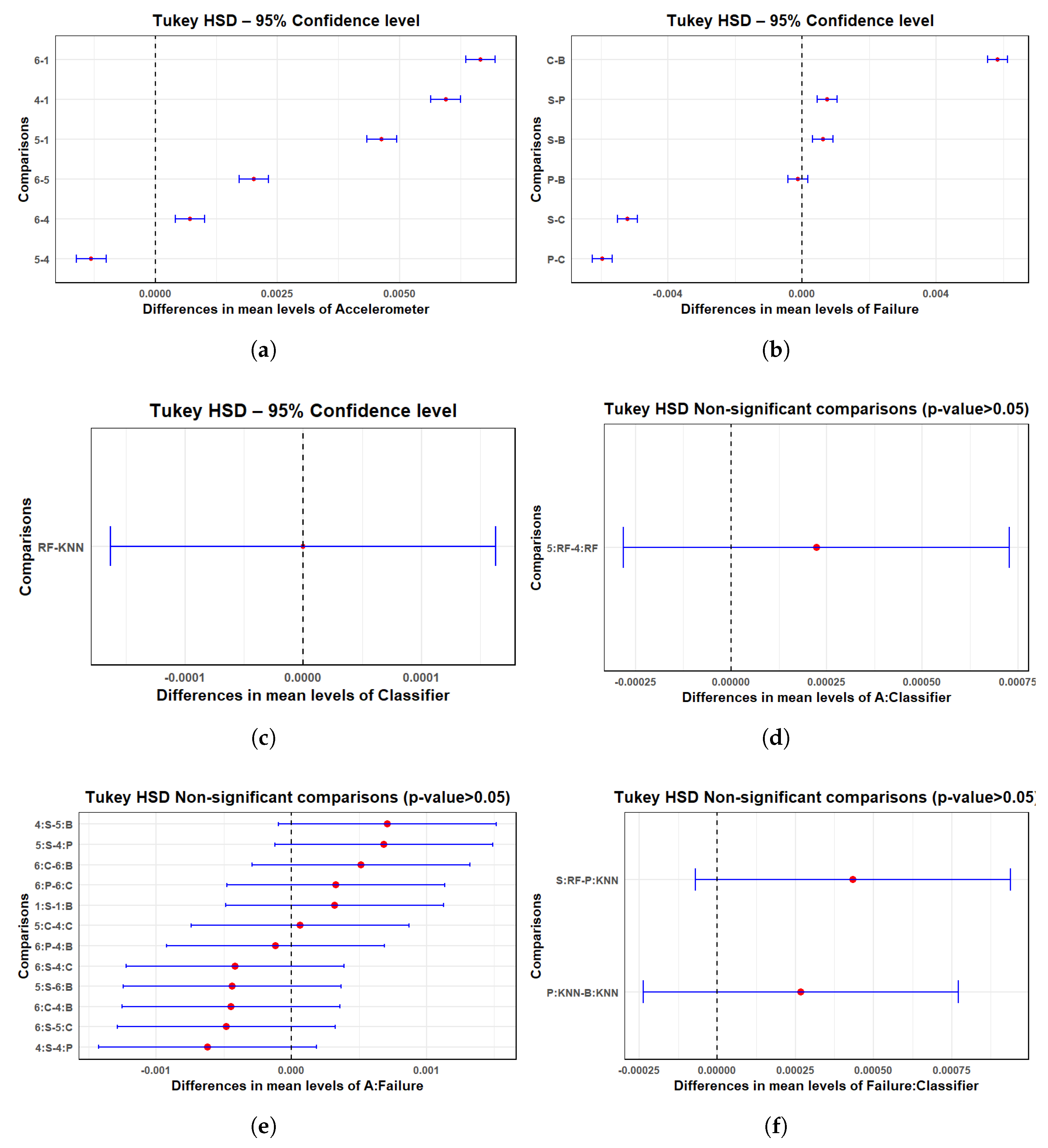
Factor	Df	Sum Square	Mean Square	F-Value	p-Value
A	3	0.2150	0.07168	1295.10	<0.001
Failure	3	0.1954	0.06512	1176.70	<0.001
Classifier	1	0.0000	0.00000	0.00	<0.001
A:Failure	9	0.2012	0.02236	404.00	<0.001
Failure:Classifier	3	0.0762	0.02539	458.70	<0.001
A:Classifier	3	0.0184	0.00614	111.00	<0.001

Df = Degrees freedom.

.

Regarding the influence of sensor inclination, the results obtained for accelerometers A1, A2 and A3 were analysed. The ANOVA test revealed statistically significant differences (p-value < 0.001) in the average classification accuracy across the three accelerometers, the four types of failure, and the two classification models. In addition, significant interaction effects (p-value < 0.001) were observed between the accelerometer:classifier (Figure 9a), failure:classifier (Figure 9b), and accelerometer:failure (Figure 9c) factors. A summary of the ANOVA results is presented in

Table 12. ANOVA factorial test for inclination.

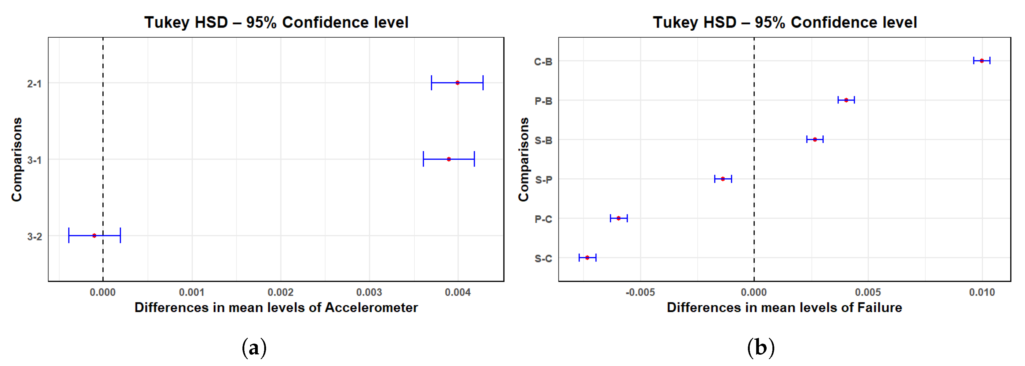
Factor	Df	Sum Square	Mean Square	F-Value	p-Value
A	2	0.0829	0.04145	680.78	<0.001
Failure	3	0.3211	0.10704	1757.89	<0.001
Classifier	1	0.0065	0.00655	107.49	<0.001
A:Failure	6	0.1427	0.02378	390.56	<0.001
Failure:Classifier	3	0.0689	0.02296	377.06	<0.001
A:Classifier	2	0.0089	0.00446	73.31	<0.001

Df = Degrees freedom.

.

Figure 10 and Figure 11 illustrate the results of Tukey’s post-hoc analyses for sensor position and inclination, respectively, highlighting the significant differences and interaction effects among the evaluated factors.As can be seen in these graphs, the differences between pairs of factor levels are practically all significant except in some cases. However, these differences are of little practical relevance as they are less than 1%, as detailed in Table 9 for the four failure types. This consideration is particularly relevant in real-world applications, where surrounding components and system attachments often limit the physical space available for sensor placement on gearboxes.

In Pichika et al. [23] and Vanrak et al. [24], a sensor’s optimum position in a gearbox when moving it along the x, y and z axes are studied and determined to extract the best information from the vibration signal. This position, although optimal, is often not accessible due to the physical layout or mounting of the gearbox. In this work, it has been determined that there are significant differences in the position and inclination of the sensor. However, the results indicate that they are of no practical importance.

4. Conclusions

In this research, a methodological proposal was made for selecting vibration signal characteristics in the time domain for a spur gearbox based on the wrapper method using RF as a classifier. The study employed a complex and realistic dataset, generated under varying motor speeds and load conditions, to better simulate real-world operating scenarios. With the proposed methodology, 7 CIs (Temporal moments higher order, Mean, Skewness, Zero crossing, Slope sign change, Energy operator and Kurtosis) were obtained, which are predominant in the four failure types: breaking, cracking, pitting and scuffing for the feature extraction process and the performance of the classification models.

By using the 7 CIs obtained in the feature selection stage in the RF and K-NN classification models, the average values of the classification accuracy of the failure severity level as well as the AUC values exceeded 98% across all six accelerometers and four failure types, indicating that the selected CIs are highly effective for analysing vibration signals and accurately determining the severity level of various failure types.

The comparison of classification accuracy values using factorial ANOVA and Tukey’s post-hoc tests revealed statistically significant differences associated with variations in sensor position and inclination. These differences, being less than 1%, are of no practical importance, so when a sensor is installed in a gearbox by moving it either along the drive shaft or the driven shaft and with some degree of inclination, the information obtained from the vibration signal will be minimally affected. The developed methodology is ideal for early detection and assessment of failure severity levels in gearboxes.

5. Future Works

Develop a multivariate statistical process control system for monitoring gearbox condition using vibration signals. Use the proposed methodology to analyse the signal acquired through the gearbox’s acoustic emission, voltage, noise, and electric current sensors.

References

- Dong, E.; Zhang, E.; Zhan, X.; Cheng, Z. A novel dynamic predictive maintenance framework for gearboxes utilizing 341 nonlinear Wiener process. Meas. Sci. Technol. 2024, 35, 126210. [Google Scholar] [CrossRef]
- Goswami, P.; Rai, R.N. A systematic review on failure modes and proposed methodology to artificially seed faults for promoting PHM studies in laboratory environment for an industrial gearbox. Eng. Fail. Anal. 2023, 146, 107076. [Google Scholar] [CrossRef]
- Cerrada, M.; Zurita, G.; Cabrera, D.; Sánchez, R.V.; Artés, M.; Li, C. Fault diagnosis in spur gears based on genetic algorithm and random forest. Mech. Syst. Signal Process. 2016, 70, 87–103. [Google Scholar] [CrossRef]
- Pérez-Torres, A.; Sánchez, R.V.; Barceló-Cerdá, S. Selection of the level of vibration signal decomposition and mother wavelets to determine the level of failure severity in spur gearboxes. Qual. Reliab. Eng. Int. 2024, 40, 3439–3451. [Google Scholar] [CrossRef]
- Sendlbeck, S.; Fimpel, A.; Siewerin, B.; Otto, M.; Stahl, K. Condition monitoring of slow-speed gear wear using a transmission error-based approach with automated feature selection. Int. J. Progn. Health Manag. 2021, 12. [Google Scholar] [CrossRef]
- Seo, M.K.; Yun, W.Y. Gearbox Condition Monitoring and Diagnosis of Unlabeled Vibration Signals Using a Supervised Learning Classifier. Machines 2024, 12, 127. [Google Scholar] [CrossRef]
- Sharma, V.; Parey, A. A review of gear fault diagnosis using various condition indicators. Procedia Eng. 2016, 144, 253–263. [Google Scholar] [CrossRef]
- Hızarcı, B.; Ümütlü, R.C.; Kıral, Z.; Öztürk, H. Fault severity detection of a worm gearbox based on several feature extraction methods through a developed condition monitoring system. SN Appl. Sci. 2021, 3, 129. [Google Scholar] [CrossRef]
- Salameh, J.P.; Cauet, S.; Etien, E.; Sakout, A.; Rambault, L. Gearbox condition monitoring in wind turbines: A review. Mech. Syst. Signal Process. 2018, 111, 251–264. [Google Scholar] [CrossRef]
- Sanchez, R.V.; Lucero, P.; Vásquez, R.E.; Cerrada, M.; Macancela, J.C.; Cabrera, D. Feature ranking for multi-fault diagnosis of rotating machinery by using random forest and KNN. J. Intell. Fuzzy Syst. 2018, 34, 3463–3473. [Google Scholar] [CrossRef]
- Wang, J.; Li, S.; Xin, Y.; An, Z. Gear fault intelligent diagnosis based on frequency-domain feature extraction. J. Vib. Eng. Technol. 2019, 7, 159–166. [Google Scholar] [CrossRef]
- Vakharia, V.; Gupta, V.K.; Kankar, P.K. A comparison of feature ranking techniques for fault diagnosis of ball bearing. Soft Comput. 2016, 20, 1601–1619. [Google Scholar] [CrossRef]
- Nayana, B.; Geethanjali, P. Analysis of statistical time-domain features effectiveness in identification of bearing faults from vibration signal. IEEE Sens. J. 2017, 17, 5618–5625. [Google Scholar] [CrossRef]
- Lei, Y.; Zuo, M.J. Gear crack level identification based on weighted K nearest neighbor classification algorithm. Mech. Syst. Signal Process. 2009, 23, 1535–1547. [Google Scholar] [CrossRef]
- Patel, D.; Saxena, A.; Wang, J. A Machine Learning-Based Wrapper Method for Feature Selection. Int. J. Data Warehous. Min. (IJDWM) 2024, 20, 1–33. [Google Scholar] [CrossRef]
- Liu, Z.; Zhao, X.; Zuo, M.J.; Xu, H. Feature selection for fault level diagnosis of planetary gearboxes. Adv. Data Anal. Classif. 2014, 8, 377–401. [Google Scholar] [CrossRef]
- Maseno, E.M.; Wang, Z. Hybrid wrapper feature selection method based on genetic algorithm and extreme learning machine for intrusion detection. J. Big Data 2024, 11, 24. [Google Scholar] [CrossRef]
- Efron, B.; Tibshirani, R.J. An Introduction to the Bootstrap; CRC Press: Boca Raton, FL, USA, 1994. [Google Scholar] [CrossRef]
- Raschka, S. Model evaluation, model selection, and algorithm selection in machine learning. arXiv 2018, arXiv:1811.12808. [Google Scholar] [CrossRef]
- Caesarendra, W.; Widodo, A.; Yang, B.S. Combination of probability approach and support vector machine towards machine health prognostics. Probabilistic Eng. Mech. 2011, 26, 165–173. [Google Scholar] [CrossRef]
- Shandhoosh, V.; Venkatesh S, N.; Chakrapani, G.; Sugumaran, V.; Ramteke, S.M.; Marian, M. Intelligent fault diagnosis for tribo-mechanical systems by machine learning: Multi-feature extraction and ensemble voting methods. Knowl.-Based Syst. 2024, 305, 112694. [Google Scholar] [CrossRef]
- Guo, K.; Wan, X.; Liu, L.; Gao, Z.; Yang, M. Fault diagnosis of intelligent production line based on digital twin and improved random forest. Appl. Sci. 2021, 11, 7733. [Google Scholar] [CrossRef]
- Pichika, S.N.; Yadav, R.; Rajasekharan, S.G.; Praveen, H.M.; Inturi, V. Optimal sensor placement for identifying multi-component failures in a wind turbine gearbox using integrated condition monitoring scheme. Appl. Acoust. 2022, 187, 108505. [Google Scholar] [CrossRef]
- Vanraj; Dhami, S.; Pabla, B. Optimization of sound sensor placement for condition monitoring of fixed-axis gearbox. Cogent Eng. 2017, 4, 1345673. [Google Scholar] [CrossRef]
- Islam, M.S.; Kim, K.; Kim, H.Y. Data-Driven Approach for Fault Diagnosis of Harmonic Drives Using Wireless Acceleration Sensors and Machine Learning. Int. J. Precis. Eng. Manuf.-Green Technol. 2025, 12, 951–968. [Google Scholar] [CrossRef]
- Asutkar, S.; Tallur, S. An explainable unsupervised learning framework for scalable machine fault detection in Industry 4.0. Meas. Sci. Technol. 2023, 34, 105123. [Google Scholar] [CrossRef]
- Rigas, S.; Papachristou, M.; Sotiropoulos, I.; Alexandridis, G. Explainable Fault Classification and Severity Diagnosis in Rotating Machinery Using Kolmogorov–Arnold Networks. Entropy 2025, 27, 403. [Google Scholar] [CrossRef]
- Palaniappan, R. Comparative analysis of support vector machine, random forest and k-nearest neighbor classifiers for predicting remaining usage life of roller bearings. Informatica 2024, 48, 39–52. [Google Scholar] [CrossRef]
- Du, P.; Abdel Jabbar, N.M.; Wilhite, B.A.; Kravaris, C. Fault Diagnosis in Chemical Reactors with Data-Driven Methods. Ind. Eng. Chem. Res. 2025, 64, 6060–6076. [Google Scholar] [CrossRef]
- Breiman, L. Random forests. Mach. Learn. 2001, 45, 5–32. [Google Scholar] [CrossRef]
- Dudani, S.A. The Distance-Weighted k-Nearest-Neighbor Rule. IEEE Trans. Syst. Man Cybern. 1976, SMC-6, 325–327. [Google Scholar] [CrossRef]
- Yu, Z.; Chen, H.; Liu, J.; You, J.; Leung, H.; Han, G. Hybrid k-Nearest Neighbor Classifier. IEEE Trans. Cybern. 2016, 46, 1263–1275. [Google Scholar] [CrossRef] [PubMed]
- Prasath, V.; Alfeilat, H.A.A.; Hassanat, A.; Lasassmeh, O.; Tarawneh, A.S.; Alhasanat, M.B.; Salman, H.S.E. Distance and Similarity Measures Effect on the Performance of K-Nearest Neighbor Classifier—A Review. arXiv 2017, arXiv:1708.04321. [Google Scholar] [CrossRef]
- Bradley, A.P. The use of the area under the ROC curve in the evaluation of machine learning algorithms. Pattern Recognit. 1997, 30, 1145–1159. [Google Scholar] [CrossRef]
- R Core Team. R: A Language and Environment for Statistical Computing; R Foundation for Statistical Computing: Vienna, Austria, 2024. [Google Scholar]
- Choi, E.; Lee, C. Feature extraction based on the Bhattacharyya distance. Pattern Recognit. 2003, 36, 1703–1709. [Google Scholar] [CrossRef]
- Rencher, A.C. Multivariate Statistical Inference and Applications; Wiley: New York, NY, USA, 1998; Volume 635. [Google Scholar]
- Patel, R.K.; Giri, V. Feature selection and classification of mechanical fault of an induction motor using random forest classifier. Perspect. Sci. 2016, 8, 334–337. [Google Scholar] [CrossRef]