Transformation of Coordinates of Boundary Points of Neighboring Mining Areas Using an Authorial Procedure Based on the Method of Independent Models—A Case Study

Abstract

In order to integrate data relevant to decision making, especially for the development of post-mining areas, it is important to ensure their uniform spatial reference. A problem arises when the coordinates of the boundary points of mining areas of neighboring mines are documented in different local rectangular flat coordinate systems. It is then necessary to transform the coordinates of these points into a uniform coordinate system. The currently implemented coordinate transformations in Poland, which are implemented separately for each area, do not allow the obtainment of the equal coordinates of identical boundary points. Therefore, topological consistency in such areas is missing. This problem was the focus of the research carried out by the authors. An authorial transformation procedure has been developed based on the method of independent models, which makes it possible to obtain the equal coordinates of identical boundary points using the transformation procedure. This procedure is presented in this article. The results of the transformation of the coordinates of boundary points of 14 mining areas located in the southern part of Poland, i.e., in the Upper Silesian Coal Basin, are also presented in this article. This task was carried out using the previously used transformation, performed separately for each of the mining areas and in accordance with the authorial procedure presented in this article. It was found that the values of differences in the locations of identical boundary points of the areas after the execution of separate transformation ranged from 0.002 m to 1.945 m. The difference in coordinates Δx and Δy reached a maximum value of 1.937 m and 0.542 m, respectively. The differences in the coordinates of identical boundary points, using the method of independent models, reached a maximum value of 0.001 m, which basically resulted from the rounding up of significant figures. The above facts indicate the validity of using the solution proposed by the authors, allowing topological consistency in areas where it is necessary to integrate the spatial data of neighboring areas.

1. Introduction

One of the greatest challenges facing civilization today is to stop the climate crisis through transformation and achieve climate neutrality. In response to this challenge, Poland is implementing a European Union (EU) strategy for a stable energy union based on a forward-looking climate policy, in order to achieve EU climate neutrality by 2050. Measures to be undertaken in this area will be executed over many years. They are included in the strategic transformation document entitled the National Energy and Climate Plan until 2030, which sets the directions for Poland’s transformation. Decarbonization efforts are planned to be accelerated. Coal mining and coal-based energy constitute a relatively large segment of the national economy. For many years, hard coal has been the basis for meeting the demand for primary energy in Poland. The use of coal is currently being gradually replaced by zero-emission fuels. As a result, an increasing number of hard coal mines are being closed, and most of the coal mines in Poland are expected to be closed by 2030. The largest part of domestic hard coal extraction involves the extraction from the Upper Silesian Coal Basin (USCB). Mining operations and mine closures are accompanied by numerous hazards, including water and gas hazards, continuous and discontinuous surface deformations in the form of sinkholes, or post-mining seismicity. These issues are presented, among others, in references [1,2,3]. In order to correctly assess the possibility of such hazards and to take actions to limit the effects of the hazards, and consequently to make decisions regarding the development of such areas in the conditions ensuring public safety, it is important to have reliable and comprehensive information on mining operations conducted in these areas in the past. The correct spatial location is crucial here. The problem is that the geological and survey documentation processes of mines were basically carried out in local rectangular flat coordinate systems, and due to the necessity to implement the provisions of the Directive of the European Parliament and of the Council establishing an Infrastructure for Spatial Information in the European Community (INSPIRE) in Poland [4], based on the transposition of the Directive into the provisions of national law, through the Act on the Infrastructure of Spatial Information [5], it became mandatory to use coordinate systems that are an element of the national spatial reference system [6,7]. In the legal acts concerning mining activities [8], or geological and survey documentation [9], provisions were incorporated allowing the maintenance of geological and survey documentation in local coordinate systems, provided that the mining plant ensures the possibility of its transformation to the national system (currently PL-2000). Cartographic documentation was or is still maintained in the following coordinate systems: Sucha Góra (the variants 1885, 1901, 1923, 1926, ROW-Rybnik Coal Area, GOP-Upper Silesian Industrial Region), Borowa Góra, 1965, S-JTSK (System of the Unified Trigonometrical Cadastral Network), and KUL (Union of Lublin Mound-Lviv). For many years, the transformation task was carried out in two stages. Unfortunately, this was associated with high transformation errors. An attempt to solve this problem was made in 2017 by the Cartography and Spatial Information Systems team from the Silesian University of Technology. As a result of their studies, a new procedure was developed that allows for the transformation of coordinates directly from the local system to the national system at the required level of accuracy. Software was also developed to perform the transformation task [10,11].

The transformation problem is the subject of many other studies. In reference [12], the author discusses transformations between different coordinate systems currently used in Australia. Some practical solutions to the problem of transformation between local geodetic coordinate systems, as well as between the local geodetic system and global reference systems, are described in reference [13]. In reference [14], the problem involving the transformation of cadastral map coordinates to the national coordinate system in Turkey is presented. The importance of a correct procedure for the transformation task is discussed in reference [15]. A solution for improving the precision of coordinate transformation using the classification and weighting of coordinate components is provided in reference [16]. A new method for calculating transformation parameters and assessing the precision of transformation is presented in reference [17]. The importance of correct coordinate transformation for monitoring surface deformations is presented in reference [18]. Moreover, when using Interferometric Synthetic Aperture Radar (InSAR) [19] and Light Detection and Ranging (LiDAR) [20] technology, it is essential to execute the transformation task correctly.

The problem of coordinate transformation has been the subject of a number of studies carried out for the area of the Czech Republic. Reference [21], concerning the Karvina-Ostrava Coal District, indicated the optimum transformation relations that disallow interfering with the accuracy of calculations and measurements obtained in the Otto coordinate system. In reference [22], the authors present the results of a study on inter-system transformations for the georeferencing of old mine workings. Furthermore, the basic features of the transformation between the analyzed systems to obtain coordinates in the European Terrestrial Reference System were defined.

The research conducted by the authors of this article has shown that a significant problem of transformation carried out independently (separately) for each mining area involves finding the different coordinates of identical points in the national coordinate system, which is particularly important in the case of boundary points of neighboring mines. Therefore, there is a lack of topological consistency in these areas. The above-mentioned problem prevents the appropriate integration of spatial data at the municipal, provincial, and national level, which is important for making decisions on spatial planning and management, including the appropriate management of mining and post-mining areas. This problem was the subject of the research continued by the authors (including [23]). An authorial transformation procedure based on the method of independent models (MIM) has been developed. The method is used in photogrammetry, and more precisely in aerotriangulation. The first mentions of the method appeared in the 1920s with the beginning of the development of an independent model of air triangulation. The principles of this method were discussed in the article by H.G. Fourcade [24]. E.H. Thomson in their work [25] emphasized the contribution of H.G. Fourcade to the development of the air triangulation method. In the 1940s, solutions related to independent models reappeared (e.g., [26]). The research described in references [27,28] allowed for the robust development of MIM. The 1970s were a period when independent models were considered superior to non-iterative methods [29]. In later years, the method of independent models was used in various areas. The studies mentioned in references [30,31] are noteworthy, where the authors indicate the possibilities of using MIM to build 3D models and the advantages of this method in this field. In Poland, studies related to this topic were described in references [32,33,34,35].

A new application of MIM in relation to the transformation of the coordinates of boundary points of neighboring areas is presented in this article. The procedure and results of the transformation task of the coordinates of boundary points of 14 mining areas located in the southern part of Poland, i.e., in the Upper Silesian Coal Basin, are presented. This task was carried out using a single-stage conformal transformation of the first degree, performed separately for each of the mining areas, in order to demonstrate the validity of the solution proposed by the authors.

2. Materials and Methods

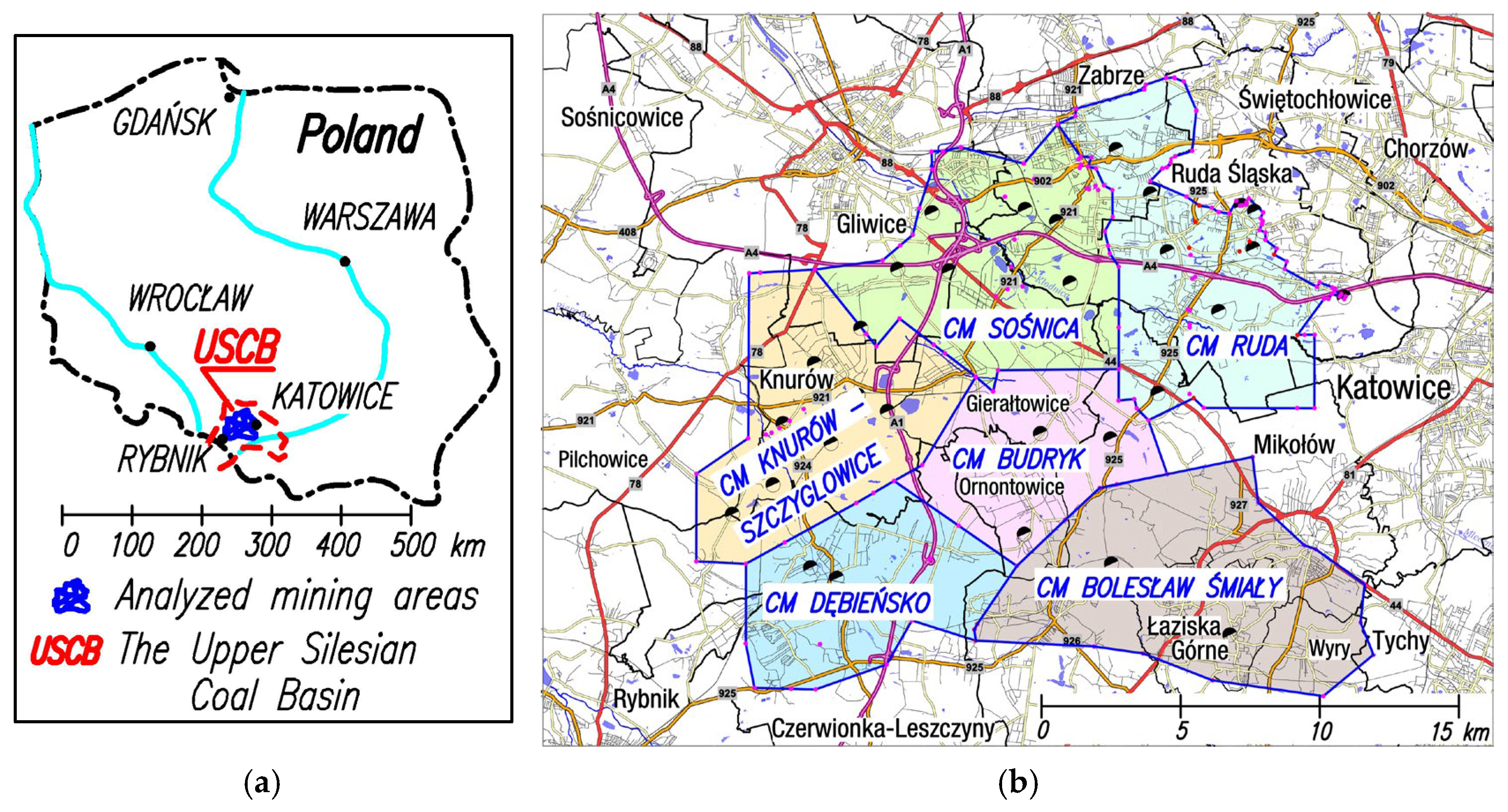
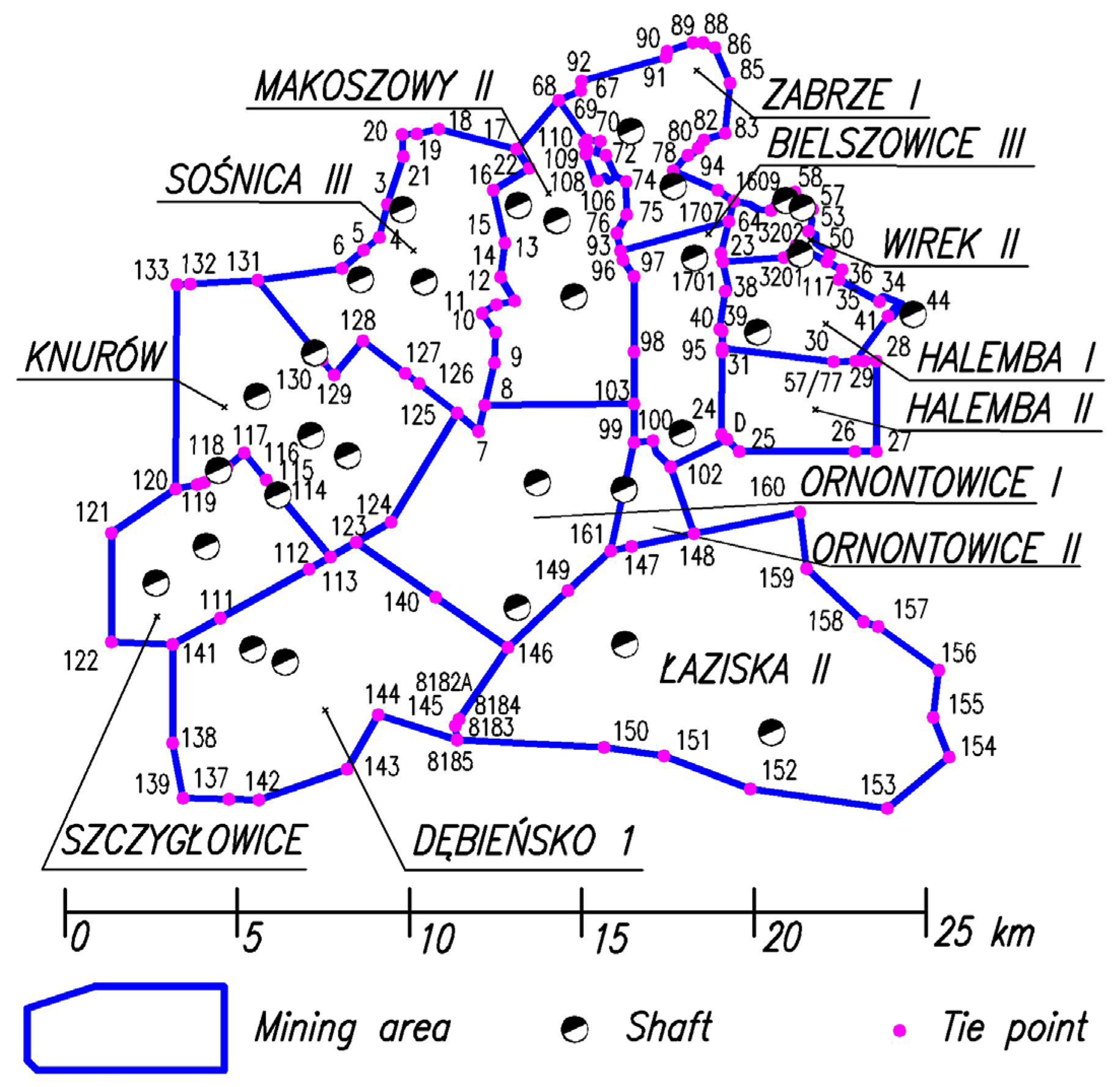
2.1. Location of the Study Area and Source Materials

The research on the subject of study was conducted in the Upper Silesian Coal Basin. This area is located in the southern part of Poland and in the Ostrava-Karviná region in the Czech Republic (Figure 1a). The total area of the basin is approximately 7250 km², including approximately 5600 km² in Poland. The total area of the documented deposits in this area is over 3049 km². Currently, 80.06% of the documented balance resources of Polish hard coals are located in this basin. The research was carried out for the areas of hard coal mines (active, closed, or in the process of being closed) adjacent to each other, located in the Polish part of the Upper Silesian Coal Basin (Figure 1b). A total of 14 mining areas of the above-mentioned mines were studied. For the purposes of implementing the transformation task, the coordinates of the boundary points of the above-mentioned mining areas and shafts located in individual areas were collected. The coordinates of boundary points were obtained in the local system (Sucha Góra 1901, 1926—Bessel ellipsoid), while the coordinates of shafts were obtained in the local system (Sucha Góra, 1901, 1926) and in the national system (PL-2000—GRS 80 ellipsoid). The data were made available by the State Mining Office (SMO) and the SMO Documentation Archive. Overall, the data were collected for 248 boundary points and 52 shafts. Figure 2 shows the boundaries of mining areas with boundary points (tie points) and the location of shafts.

Table 1. Summary of the analyzed mining areas.

No.	Name of Coal Mine (CM)	Name of Mining Area	Number of Boundary Points (Tie Points)	Number of Adjustment Points (Shafts)
1	CM Bolesław Śmiały	Łaziska II	18	3
2	CM Budryk	Ornontowice I	11	4
3	CM Budryk	Ornontowice II	7	1
4	CM Dębieńsko	Dębieńsko 1	19	2
5	CM Knurów-Szczygłowice	Knurów	19	8
6	CM Knurów-Szczygłowice	Szczygłowice	13	5
7	CM Sośnica	Makoszowy II	28	5
8	CM Ruda	Bielszowice III	18	6
9	CM Ruda	Zabrze I	30	3
10	CM Ruda	Halemba I	15	5
11	CM Ruda	Halemba II	9	-
12	CM Ruda	Halemba-East Shaft	10	1
13	CM Ruda	Wirek II	24	3
14	CM Sośnica	Sośnica III	27	6

contains information on the affiliation of individual areas to hard coal mines.

2.2. Methodology

As part of the research, the results of which are presented in the article, the transformation task of the boundary points of the neighboring mining areas was carried out using a single-stage conformal transformation of the first degree performed separately for each of the mining areas and in accordance with the developed authorial procedure, using the method of independent models. The task using a single-stage (separate) transformation was carried out in order to demonstrate that this is not a transformation that ensures the attainment of equal coordinates of identical boundary points. In the research conducted using both methods, the separate transformation and the method of independent models, “adjustment points” (in this research called shafts) are understood as points with known coordinates both in the local rectangular flat coordinate system and in the national system. In both methods, “tie points” are understood as boundary points. The difference is that, in the separate method, tie points do not affect the calculation of transformation coefficients. They are only used to calculate the extent of shift in the neighboring areas, which occur as a result of the separate transformation of each of these areas.

2.2.1. Single-Step Transformation—Separate

The transformation from the local system (Sucha Góra) to the national system PL-2000, separately for each mining area in the subject area, was performed using a single-stage, first-degree conformal transformation. The transformation parameters were determined based on the coordinates of points (shafts) in both systems (local and national), in accordance with the procedure developed as a result of the research performed from 2017 and presented in the references [10,11]:

-

The selection and analysis of adjustment points obtained from the mine or obtained as a result of direct field measurements.

-

The determination of the degree and type of transformation based on the adjustment points obtained from the mines. The first-degree conformal transformation (Helmert) was adopted in this research—due to the possibility to obtain transformation coefficients consistent with those currently used by the mine.

The equations in the matrix notation are expressed as follows (1):

$$\left[\begin{array}{c}X\\ Y\end{array}\right]=\left[\begin{array}{c}{t}_X\\ t_Y\end{array}\right]+m\left[\begin{array}{cc}cos\varphi & -sin\varphi \\ sin\varphi & cos\varphi \end{array}\right]\left[\begin{array}{c}x\\ y\end{array}\right]$$

(1)

where

X—coordinate x in the secondary (national) system;

Y—coordinate y in the secondary (national) system;

x—coordinate x in the primary (local) system;

y—coordinate y in the primary (local) system;

t_X—the shift (translation) vector in the x direction;

t_Y—the shift (translation) vector in the y direction;

m—the transformation scale change factor;

ϕ—the rotation angle of the coordinate system axes;

$\left[\begin{array}{cc}cos\varphi & -sin\varphi \\ sin\varphi & cos\varphi \end{array}\right]$—the rotation matrix.

-

Comparison of the coordinates of the adjustment points with the coordinates obtained from the transformation. The verification process should include the calculation of the differences in the x and y coordinates and the resultant difference. If the deviation exceeds the assumed maximum error values, then the transformation parameters should be re-determined.

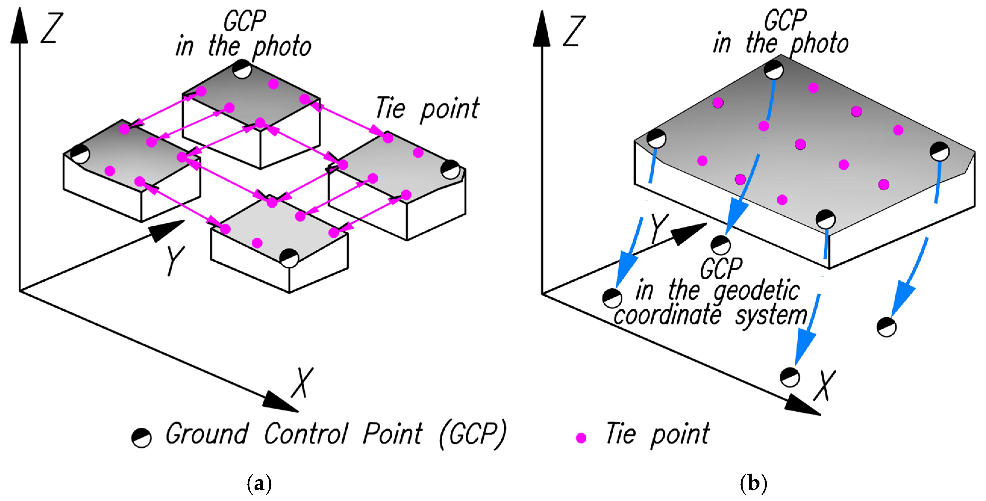
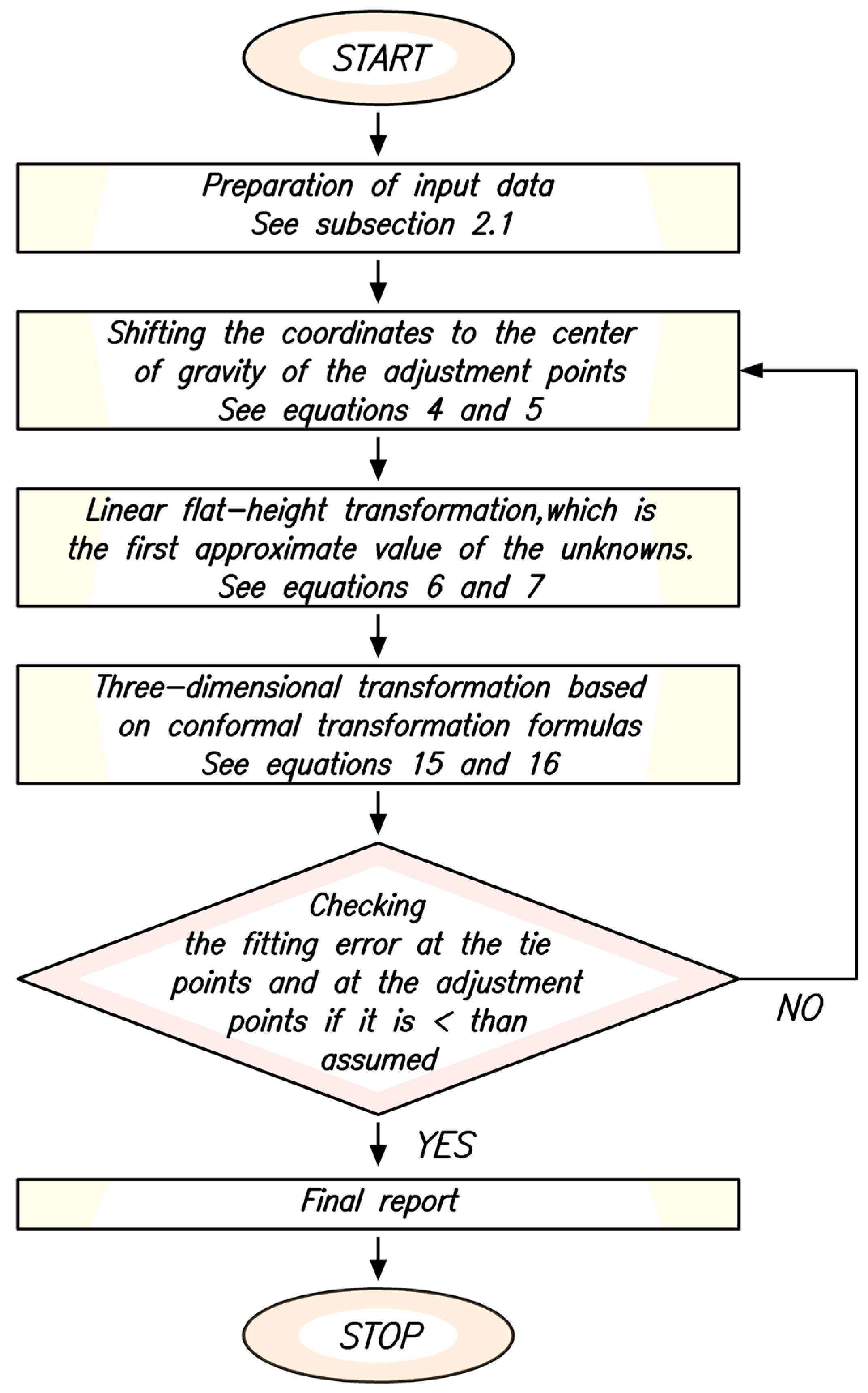
2.2.2. Transformation Using the Authorial Procedure Based on the Method of Independent Models

As already mentioned, the method of independent models (MIM) is used, among others, in photogrammetry. Photogrammetric photos can be processed using the aerotriangulation method. We can distinguish block aerotriangulation from independent models and block aerotriangulation from independent photos. The method of independent models consists of building units from pairs of photos. Each model is built in an independent spatial coordinate system. The models are then combined in the alignment process.

The standard input data are the spatial coordinates of the model points built as a result of the mutual orientation of the pairs of photos. The coordinates of the tie points, photo points, and centers of photo projections are incorporated into the model. The tie points allow for combining photos into blocks. Photo points are points with measured ground coordinates, which are visible in the photos. They allow for the perpendicular stabilization of the photos. By including the centers of the photo projections, a height stabilization of the block along the rows can be obtained. Aerotriangulation can be understood as a process of simultaneous transformation of all models to one coordinate system. For this purpose, a spatial conformal transformation is used. The transformation parameters include model rotation parameters, translation coefficients, and a scale factor. It is necessary to determine seven parameters in order to connect the models and cover the photo points with their ground location [37]. An example of connecting independent models into an aerotriangulation block is shown in Figure 3a,b.

In the presented research, as mentioned above, it was assumed that the tie points in the implementation of the task would be identical boundary points, while the shafts would be the adjustment points (Figure 4).

In the basic procedure, the transformation task was implemented according to the algorithm presented in Figure 5.

The procedure includes the following:

I. The stage of preparing input data:

-

Obtaining the coordinates of the boundary points of mining areas and shafts located in these areas;

-

Analyzing the obtained data for completeness and quality;

-

If necessary, conducting field measurements to determine the coordinates of the shafts;

-

Preparing the appropriate input files.

II. The stage where the center of gravity of the shaft coordinates is taken into account [39]:

-

Calculating the coordinates of the center of gravity in two systems: primary (x₀, y₀) and secondary (X₀, Y₀), according to the following formulas:

$$x_0={\displaystyle \frac{\sum x_i}{n}}\hspace{1em}\hspace{1em}\hspace{1em}{y}_0={\displaystyle \frac{\sum y_i}{n}}$$

(2)

$$X_0={\displaystyle \frac{\sum X_i}{n}}\hspace{1em}\hspace{1em}\hspace{1em}{Y}_0={\displaystyle \frac{\sum Y_i}{n}}$$

(3)

where

x_i, y_i—the coordinates of points in the primary system: i = 1, 2, …, n;

X_i, Y_i—the coordinates of points in the secondary system: i = 1, 2, …, n;

n—the number of adjustment points for all i = 1, 2, …, n.

-

Shifting the coordinates to the center of gravity based on the following formulas:

$${\overline{x}}_i=x_i+x_0\hspace{1em}\hspace{1em}\hspace{1em}{\overline{y}}_i=y_i+y_0$$

(4)

$${\overline{X}}_i=X_i+X_0\hspace{1em}\hspace{1em}\hspace{1em}{\overline{Y}}_i=Y_i+Y_0$$

(5)

where

$x_i$, $y_i$—the coordinates of points in the primary system shifted to the center of gravity in the primary system;

$X_i$, $Y_i$—the coordinates of points in the secondary system shifted to the center of gravity in the secondary system;

i = 1, 2, …, n (n—the number of adjustment points).

III. The stage of linear flat-height transformation, constituting the first approximate values of unknowns. In the case of using the method of independent models for approximate fitting, height transformation is not required. It is sufficient to perform linear flat transformation.

-

In the case of points with known (adjustments) coordinates:

$$\begin{gathered} a_i+u_i · x_k^i+v_i · y_k^i=X_k+{\delta x}_k \\ {b}_i+u_i · y_k^i -v_i · x_k^i=Y_k+{\delta y}_k \end{gathered}$$

(6)

-

In case of tie points:

$$\begin{gathered} a_i+u_i · x_k^i+v_i · y_k^i-a_j-u_j · x_k^j-v_j · y_k^j={\delta x}_k^{i,j} \\ {b}_i+u_i · y_k^i-v_i· x_k^i -b_j-u_j · x_k^j+v_j · y_k^j={\delta y}_k^{i,j} \end{gathered}$$

(7)

where

$a_i$, $b_i$—the translation parameters of the i-th subset;

k—point index (point number);

i, j—the index of transformation area;

$X_k$, $Y_k$—the flat coordinates of the adjustment point in the secondary system (with the index k after shifting to the center of gravity);

$x_k^i$, $y_k^i$—the flat coordinates of the point in the i-th primary system (with the index k after shifting to the center of gravity);

u_i, v_i—the transformation parameters that are a combination of rotation ϕ and scale change.

$$s (u_i=s_i · {cos\varphi }_i, v_i=s_i · {sin\varphi }_i)$$

The above-mentioned parameters a, b, u, and v are calculated from the weighted least squares principle.

Height alignment can be performed using the following formulas:

-

In the case of points with known (adjustments) coordinates:

$$c_i+s_i · z_k^i=Z_k+{\delta z}_k^i$$

(8)

-

In the case of tie points:

$$c_i-c_j+s_i · z_k^i-s_j · z_k^j={\delta z}_k^{i,j}$$

(9)

where

$c_i$, $c_i$—the height translation (shift) of the model;

$s_i$, $s_j$—the scale change coefficients determined from the flat alignment for a given model;

$Z_k$—the height ordinate of the adjustment point (with the index k) in the secondary system after shifting to the center of gravity;

$z_k^i$, $z_k^j$—the height ordinates of the point (with index k) in the local systems of the models;

k—point index (k = 1, 2, 3, …, m, where m—the number of all points transformed in a given model);

i, j—the index of transformation area (i = 1, 2, 3, …, n, j = 1, 2, 3, …, n, where n—the number of transformation areas).

The unknown parameters of the height transformation (translation) of the models can be determined in a similar way as in the case of flat alignment.

The formulas used to calculate the approximate coordinates of points in the secondary system are as follows:

$$\begin{gathered} X_k^i=a_i+u_i · x_k^i+v_i · y_k^i \\ {Y}_k^i=b_i+u_i · y_k^i-v_i · x_k^i \\ {Z}_k^i=c_i+s_i · z_k^i \end{gathered}$$

(10)

s_i is calculated using the following formula:

$$s_i=\sqrt{u_i^2+v_i^2}$$

(11)

Explanations of parameters are analogous to those in Formulas (6)–(9).

IV. After the execution of linear flat-height transformation, a three-dimensional transformation should be performed, based on the conformal transformation formulas. It is a transformation by similarity, so it does not cause the deformation of the model shape.

-

The matrix notation of the transformation equation is expressed as follows:

$$X=\lambda ·A · x+X_0$$

(12)

where

λ—model scale change factor.

The differential nature of these transformations (small rotations, displacements, and changes in scale) is possible through appropriate conditional equations.

-

Using the so-called small rotation matrix:

$$A_m=\left|\begin{array}{ccc}1& -\delta k& \delta f\\ \delta k& 1& -\delta w\\ -\delta f& \delta w& 1\end{array}\right|$$

(13)

where

$\delta k$, $\delta f$, $\delta w$—the change in rotation angle.

-

Substituting the following values:

$$\begin{gathered} \delta k’={\delta k}_i · {\delta s}_i \\ \delta f’={\delta f}_i · {\delta s}_i \\ \delta w’={\delta w}_i · {\delta s}_i \end{gathered}$$

(14)

where

${\delta s}_i$—the change in scale for the i-th model in the next iteration;

${\delta k}_i$, ${\delta f}_i$, ${\delta w}_i$—the change in rotation angle for the i-th model in the next iteration.

-

We obtain the equations of the adjustment points (15):

$$\begin{gathered} {\delta a}_i+{\delta s}_i· x_k^i-\delta k\prime · y_k^i+\delta f\prime · z_k^i+x_k^i-X_k={\delta x}_k^i \\ {\delta b}_i+\delta k\prime · x_k^i+{\delta s}_i · y_k^i-\delta w\prime · z_k^i+y_k^i-Y_k={\delta y}_k^i \\ {\delta c}_i-\delta f\prime · x_k^i-\delta w\prime · y_k^i+{\delta s}_i · z_k^i+z_k^i-Z_k={\delta z}_k^i \end{gathered}$$

(15)

where

${\delta x}_k^i$—the apparent error of the x coordinate of the k-th point in the i-th model;

${\delta y}_k^i$—the apparent error of the y coordinate of the k-th point in the i-th model;

${\delta z}_k^i$—the apparent error of the z coordinate of the k-th point in the i-th model.

-

For the tie points, Equation (16) was used:

$$\begin{gathered} {\delta a}_i+{\delta s}_i· x_k^i-\delta k^{\prime }· y_k^i+\delta f^{\prime }· z_k^i-{\delta a}_j-{\delta s}_j· x_k^j+\delta k^{\prime } · y_k^j- \delta f^{\prime }· z_k^j ={\delta x}_k^j \\ {\delta b}_i+\delta k^{\prime }· x_k^i+{\delta s}_i· y_k^i-\delta w^{\prime }· z_k^i-{\delta b}_j-\delta k^{\prime } · x_k^j-{\delta s}_j· y_k^j+ \delta w^{\prime }· z_k^j ={\delta y}_k^j \\ {\delta c}_i-\delta f^{\prime }· x_k^i+\delta w^{\prime }· y_k^i+{\delta s}_i· z_k^i-{\delta c}_j+\delta f^{\prime } · x_k^j-\delta w^{\prime }· y_k^j+ {\delta s}_j· z_k^j ={\delta z}_k^j \end{gathered}$$

(16)

The quantities $\delta k^{\prime }$, $\delta f^{\prime }$, $\delta w^{\prime }$, $\delta s$, $\delta a$, $\delta b$, and $\delta c$ are determined using the least squares method.

-

The precise orthogonal matrix corresponding to the calculated rotations is determined from Formula (17):

$$\mathit{A}=\left|\begin{array}{ccc}cos\delta f·cos\delta k& -cos\delta f·sin\delta k& sin\delta f\\ sin\delta w·sin\delta f·cos\delta k+cos\delta w·sin\delta k& -sin\delta w·sin\delta k·sin\delta k+cos\delta w·cos\delta k& -sin\delta w·cos\delta f\\ -cos\delta w·sin\delta f·cos\delta k+sin\delta w·sin\delta k& cos\delta w·sin\delta f·sin\delta k+sin\delta w·cos\delta k& cos\delta w·cos\delta f\end{array}\right|$$

(17)

After determining the precise matrix, the coordinates are calculated according to Formula (12) as well as the agreed tie points using the arithmetic mean.

V. After the execution of three-dimensional transformation, it is necessary to check and verify the deviation at the adjustment points. When additional control points exist, it also applies to these points. If the error is greater than the assumed permissible error, we use the iterative procedure and return to the linear flat-height transformation.

VI. If the error received is acceptable, a final report is generated.

For a large area, the Earth’s curvature and the applied ellipsoid should be taken into account in the calculations. For the area in question, there was no need to use this solution because the coordinates of the secondary system points (PL-2000) in the studied area already take into account the ellipsoid. The MIM algorithm iteratively fits in or in a sense deforms the entire “aeroblock” so that it fits these target points on the ellipsoid. The Earth’s curvature, regardless of the algorithm adopted, is always taken into account. However, with such a condition, one must be aware of the occurrence of a certain systematic error, and its extent depends on the dimensions of the transformed area.

3. Results

The transformation using the separate method was performed with the application of the GEOLISP v25 [40] and GEONET 2006 [41] programs. In the case of the separate method, the transformation was performed for 11 areas meeting the transformation requirements, i.e., having the appropriate number of adjustment points (shafts). The values of deviations obtained as a result of the transformation between the Sucha Góra local systems in its various versions and PL-2000 using the separate method are presented in

Table 2. Deviations of the conformal transformation of the first degree (separate) of the flat coordinates of individual mining areas.

Name of Mining Area	Deviation Values [mm]
	Sx	Sy	S	Smax
Łaziska II	0.0	0.0	0.0	0.0
Ornontowice I	0.0	0.0	0.0	0.0
Ornontowice II	-	-	-	-
Dębieńsko 1	0.0	0.0	0.0	0.0
Knurów	0.0	0.0	0.0	0.0
Szczygłowice	1.4	1.5	2.0	2.5
Makoszowy II	0.0	0.0	0.0	0.0
Bielszowice III	2.7	2.6	3.7	6.9
Zabrze I	2.7	0.5	2.8	3.4
Halemba I	1.8	2.7	3.3	5.0
Halemba II	-	-	-	-
Halemba-East Shaft	-	-	-	-
Wirek II	1.3	3.5	3.8	4.8
Sośnica III	0.0	0.0	0.0	0.0

.

When assessing the accuracy of the transformation, the permissible transformation error in those areas was assumed to be 0.05 m.

The individual values were calculated using Formulas (18)–(20):

${Sx}_i$, ${Sy}_i$—mean square deviation:

$${Sx}_i=\sqrt{{\displaystyle \frac{\left[S{x}^2\right]}{n}}}{Sy}_i=\sqrt{{\displaystyle \frac{\left[S{y}^2\right]}{n}}}$$

(18)

S—resultant deviation (transformation error):

$$S=\sqrt{{\displaystyle \frac{\left[S{x}^2\right]+\left[S{y}^2\right]}{n-\frac{u}{2}}}}$$

(19)

u—the number of unknown transformation parameters.

Smax—the maximum resultant deviation:

$$Smax=\sqrt{(S_{xi }^2+S_{yi }^2) }$$

(20)

i = 1, 2, 3, …, n.

n—point number.

The results presented in Table 2 indicate that all the tested transformations do not exceed the permissible transformation error assumed in the work.

The transformation task was carried out using independent models in accordance with the authorial procedure [23]. The GEONET Dimensional Control software v.2020 [41] was used to perform the necessary calculations. The transformation with the use of MIM was performed for the 14 areas in question. The obtained deviations d_x and d_y of individual points were obtained in the calculation report. In the transformation using MIM, the deviations are evenly distributed over each adjustment point. In the case of the MIM transformation based on a direct transition between systems (without taking into account the curvature and ellipsoid), the deviations along x range from 0.057 m to 0.058 m, and those along the y range from 0.027 m to 0.028 m. The value of the mean square deviation was 0.064 m, which, considering the area covered by the transformation, was considered satisfactory.

The differences in the coordinates of the selected identical boundary points obtained as a result of the separate transformation and the transformation using the authorial procedure presented in the article were calculated.

${∆x}_O—$the difference in the x coordinate of the identical boundary point in the separate method;

${∆y}_O—$the difference in the y coordinate of the identical boundary point in the separate method;

${∆x}_{MIM}$—the difference in the x coordinate of the identical boundary point in MIM;

${∆y}_{MIM}—$the difference in the y coordinate of the identical boundary point in MIM;

${∆xy}_O$—the difference in the resultant xy of the same boundary point in the separate method;

${∆xy}_{MIM}—$the difference in the resultant xy of the identical boundary point in MIM.

The values of the differences in the coordinates of the identical boundary point in the separate method were calculated from Formula (21):

$${\Delta x}_O=x_{Oi}-x_{Oi}\prime \hspace{1em}\hspace{1em}\hspace{1em}{\Delta y}_O=y_{Oi}-y_{Oi}\prime$$

(21)

where

$x_{Oi}$—x coordinate of the boundary point with the i-th number in the mining area 1;

$x_{Oi}\prime$—x coordinate of the identical boundary point with the i-th number in the mining area 2;

$y_{Oi}$—y coordinate of the boundary point with the i-th number in the mining area 1;

$y_{Oi}\prime$—y coordinate of the identical boundary point with the i-th number in the mining area 2.

The values of the differences in the coordinates of the identical boundary point in the independent model method were calculated from Formula (22):

$${\Delta x}_{MIM}=x_{MIMi}-x_{MIMi}\prime \hspace{1em}\hspace{1em}{\mathsf{\Delta }y}_{MIM}=y_{MIMi}-y_{MIMi}\prime$$

(22)

where

$x_{MIMi}$—x coordinate of the i-th boundary point in the mining area 1;

$x_{MIMi}\prime$—x coordinate of the identical boundary point with the i-th number in the mining area 2;

$y_{MIMi}$—y coordinate of the boundary point with the i-th number in the mining area 1;

$y_{MIMi}\prime$—y coordinate of the identical boundary point with the i-th number in the mining area 2.

The values of the resultant difference ${\Delta xy}_O$ of the identical boundary point in the separate method were calculated from Formula (23):

$${\Delta xy}_O=\sqrt{{(x_{Oi}-x_{Oi}\prime )}^2+{(y_{Oi}-y_{Oi}\prime )}^2}$$

(23)

The values of the resultant difference Δxy_MIM of the identical boundary point in the method of independent models were calculated from Formula (24):

$${\Delta xy}_{MNM}=\sqrt{{(x_{MIMi}-x_{MIM}\prime )}^2+{(y_{MIMi}-y_{MIM} \prime )}^2}$$

(24)

Table 3. Differences in coordinates of selected identical boundary points after transformations.

Point No.	Bordering Areas	“Separate”			MIM
		${\mathbf{\Delta }\mathit{x}}_{\mathit{O}}$ [m]	${\mathbf{\Delta }\mathit{y}}_{\mathit{O}}$ [m]	${\mathbf{\Delta }\mathit{x}\mathit{y}}_{\mathit{O}}$ [m]	${\mathbf{\Delta }\mathit{x}}_{\mathit{M}\mathit{I}\mathit{M}}$ [m]	${\mathbf{\Delta }\mathit{y}}_{\mathit{M}\mathit{I}\mathit{M}}$ [m]	${\mathbf{\Delta }\mathit{x}\mathit{y}}_{\mathit{M}\mathit{I}\mathit{M}}$ [m]
8185	M.A. Łaziska II—M.A Dębieńsko 1	0.850	0.542	1.008	0.000	0.000	0.000
8184	M.A. Łaziska II—M.A. Dębieńsko 1	1.937	−0.169	1.945	0.000	0.000	0.000
8183	M.A. Łaziska II—M.A. Dębieńsko 1	1.001	0.061	1.003	0.000	0.000	0.000
8182A	M.A. Łaziska II—M.A. Dębieńsko 1	0.735	0.210	0.765	−0.001	−0.001	0.001
8181	M.A. Łaziska II—M.A. Dębieńsko 1	0.860	0.217	0.887	−0.001	0.001	0.001
8181	M.A. Łaziska II—M.A. Ornontowice I	0.886	0.197	0.908	−0.001	0.000	0.001
9461	M.A. Łaziska II—M.A. Ornontowice I	0.794	0.210	0.821	0.000	−0.001	0.001
8182	M.A. Łaziska II—M.A. Ornontowice I	0.729	0.218	0.761	0.000	0.001	0.001
8181	M.A. Dębieńsko 1—M.A. Ornontowice I	0.026	−0.020	0.032	0.000	−0.001	0.001

contains a fragment of the calculation results.

In order to evaluate the obtained results, basic statistical measures were calculated: Min_ΔX (the minimum absolute difference of x coordinates), Max_ΔX (the maximum absolute difference of y coordinates), σ_ΔX (the standard deviation of the differences in x coordinates), Min_ΔY (the minimum absolute difference in y coordinates), Max_ΔY (the maximum absolute difference in yY coordinates), σ_ΔY (the standard deviation of the differences in y coordinates), Min_ΔXY (the minimum resultant difference), and σ_ΔXY (the standard deviation of resultant differences). The results are presented in

Table 4. Differences in coordinates of identical boundary points after performing separate transformation.

MinΔx [mm]	MaxΔx [mm]	${\mathsf{\sigma }}_{\mathbf{\Delta }\mathit{X}}$ [mm]	MinΔy [mm]	MaxΔy [mm]	${\mathsf{\sigma }}_{\mathbf{\Delta }\mathit{Y}}$ [mm]	MinΔxy [mm]	MaxΔxy [mm]	${\mathsf{\sigma }}_{\mathbf{\Delta }\mathit{X}\mathit{Y}}$ [mm]
0.00	1937.00	417.89	0.00	542.00	81.76	2.00	1945.00	349.23

and

Table 5. Differences in coordinates of identical boundary points after transformation using MIM.

MinΔx [mm]	MaxΔx [mm]	${\mathsf{\sigma }}_{\mathbf{\Delta }\mathit{X}}$ [mm]	MinΔy [mm]	MaxΔy [mm]	${\mathsf{\sigma }}_{\mathit{\Delta }\mathit{Y}}$ [mm]	MinΔxy [mm]	MaxΔxy [mm]	${\mathsf{\sigma }}_{\mathbf{\Delta }\mathit{X}\mathit{Y}}$
0.00	1.00	0.55	0.00	1.00	0.55	0.00	1.00	1.00

.

The values of the differences in location between the identical boundary points of the areas after the execution of conformal transformation of the first degree (separate) range from 0.002 m to 1.945 m. The standard deviation of the differences in the location was approximately 0.349 m. The difference in the coordinates Δx and Δy reached a maximum value of approximately 1.937 m and 0.542 m, respectively. On the other hand, the differences in the coordinates of identical boundary points, using the method of independent models, reached a maximum value of 0.001 m in the entire analyzed set.

Figure 6 presents the quantitative distribution of the number of identical boundary points in relation to the differences in their location after the transformation in seven class intervals: I—(0 m–0.010 m); II—(0.010 m–0.025 m); III—(0.025 m–0.050 m); IV—(0.05 m–0.10 m); V—(0.1 m–0.5 m); VI—(0.5 m–1.0 m); and VII—(1.0 m–2.0 m).

Based on the distribution shown in Figure 6, it was found that, in the case of about 60% of the boundary points, the differences were not greater than 0.05 m, and in the remaining approximately 40% of cases, the differences were within the range from 0.05 m to as much as about 2 m. However, in as many as 32 cases, the differences were above 0.50 m.

The above facts allow us to state that the method developed as a result of the research using independent models is much more advantageous from the perspective of the implementation of the transformation, with the assumed need to obtain the same coordinates of identical boundary points. Due to the fact that the differences in coordinates of a maximum value of 0.001 m result from the rounding up of significant figures, it can be assumed that the transformation procedure presented in the article ensures the acquisition of equal values of identical boundary points.

4. Discussion

The problem presented in this article, concerning the implementation of the transformation of identical boundary points of neighboring mining areas, is of key importance, especially in post-mining areas, particularly in the period of mine liquidation. It should be noted that, both in closed areas and active mines, numerous threats are observed, including the threat of surface deformation and water or seismic hazards, and the correct assessment of the possibility of such threats is crucial for making decisions regarding their management, which would ensure public safety. This is related, among other things, to the access to information on the coordinates of the boundary points of mining areas, especially the neighboring ones, where these coordinates were documented using local rectangular flat coordinate systems, and the implementation of tasks at the municipal, provincial, or national level requires access to spatial information in one binding national coordinate system. Therefore, the above fact necessitates the transformation of coordinates from the local system to the national one, including the coordinates of the boundary points of the mining areas that are adjacent to each other.

Another problem is the fact that, in the currently used solutions involving the implementation of the transformation task separately for each mining area, there is a lack of topological consistency, despite the fact that the transformation errors meet the current accuracy criteria, i.e., they do not exceed the transformation error of 0.05 m (Table 2). The minimum value of the transformation error is 0 m and the maximum value is approximately 0.04 m. The calculated coordinate differences in selected identical boundary points after transformations performed separately for each mining area are included in Table 3. The summary of basic statistical measures covering the full range of transformed points is presented in Table 4. The values of the differences in the position of identical boundary points in the analyzed areas after the transformation ranged from 0.002 m to 1.945 m, the standard deviation of the differences in the position was about 0.349 m, and the difference in the coordinates Δx and Δy reached a maximum value of about 1.937 m and 0.542 m, respectively (Table 4). The analysis of the distribution of differences in individual classes indicated that, in as many as 40% of cases, the differences in location exceeded the value of 0.05 m, and in 32 cases, they ranged from 0.50 m to about 2.00 m (Figure 6). The above situation absolutely eliminates the possibility of a correct assessment of the location of the occurrence of post-mining hazards and, consequently, their safe development.

This article presents an authorial procedure for the implementation of the transformation task based on the method of independent models that eliminates the above-mentioned problem. The transformation errors also meet the assumed accuracy requirements, and the differences in the coordinates of identical boundary points, when using the method of independent models, reach a maximum value of 0.001 m in the entire analyzed set. The standard deviation of the differences in position was also about 0.001 m, while both the difference in coordinates Δx and Δy reached a maximum value of only 0.001 m.

The analysis showed that this resulted from the rounding up of significant figures. At the same time, it can be assumed that the transformation procedure developed in this study ensures the acquisition of equal values of identical boundary points.

For the developed procedure, it does not matter what local coordinate system is used in a given area (it does not matter whether the input coordinates are in the Sucha Góra, Borowa Góra, 1965 systems, etc.). Even several systems (also in one mine) can be aligned simultaneously—each system is a separate transformation area—and it does not matter whether the areas overlap.

The separate transformation method results in boundary points that have identical coordinates before the transformation, but after the transformation, their coordinates differ. In areas where there are no adjustment points or a non-exhaustive number of them, it is not possible to use the separate transformation, or the transformation runs without control. The method of independent models ensures that there are no errors in the topology of the areas. The simultaneous use of all data provides a large number of redundant observations, which allow gross errors to be found and eliminated.

Basically, using the independent model method requires a transformation of planes parallel to each other. In this study, the span of the area covered by the transformation is about 27 km, and the angle of inclination of the most distant planes reaches a value of only 20′ relative to each other; therefore, additionally taking into account a small number of transformed points compared to the typical photogrammetric calculations, the parallelism of the planes is obtained through the iterative procedure included in the discussed transformation procedure.

The proposed procedure can be successfully applied to small areas, such as that of this study, where the total area was 420 km² and the maximum span was about 27 km. It can be assumed that the curvature of the Earth, regardless of the adopted algorithm, is always taken into account. The coordinates of the points of the secondary system (PL-2000) are based on the GRS 80 ellipsoid. The MIM algorithm iteratively fits the entire “aeroblock” to these target points on the ellipsoid. On the other hand, for a large area, the ellipsoid used should be taken into account in the calculations. The authors also developed a procedure based on MIM, which will be presented in a separate publication. The above facts allow us to state that the method using independent models developed in our research, with the assumed need to obtain the same coordinates of identical boundary points, is significantly advantageous from the implementation perspective of the transformation.

5. Summary and Conclusions

This article presents a method for solving a significant problem involving the lack of agreement of the coordinates of identical boundary points of neighboring areas, which appears in relation to the transformation of coordinates between different systems. This study involves the boundary points of neighboring mining areas located in Poland in the Upper Silesian Coal Basin region. The significance of this problem in relation to the safe development of post-mining areas is indicated.

Based on the presented analyses, it can be stated that the authorial procedure proposed in this article, using the method of independent models, allows the obtainment of consistent coordinates of identical boundary points. In the presented case, differences of only 0.001 m were found, which result from the rounding up of significant figures. Its application in the presented example allowed the elimination of differences in the coordinates of identical boundary points of the order of even several meters.

The procedure allows us to fulfill the condition of topological agreement and can also be successfully applied in the cases of transformation of coordinates of other neighboring areas. It should be noted that its application is determined by the total size of the area undergoing transformation. However, for a large area, the applied curvature of the Earth and the ellipsoid should be taken into account in the calculations. Therefore, the authors have also developed a similar procedure that takes into account the curvature of the Earth, based on the MIM. This procedure will be presented in a separate publication.

References

1. Sokoła-Szewioła, V.; Kotyrba, A.; Alheib, M. Methods on Assessment and Monitoring of Seismic Hazards in Coal Post-Mining Areas Guidelines; Sokoła-Szewioła, V., Kotyrba, A., Alheib, M., Eds.; Silesian University of Technology Publishing House: Gliwice, Poland, 2023; p. 117. Available online: https://delibra.bg.polsl.pl/Content/77017/Methods-on-assessment-and-monitoring-of-seismic-hazards_2023.pdf (accessed on 5 May 2025).
2. Dominique, P.; Aochi, H.; Morel, J. Triggered seismicity in a former flooded coal mining basin (Gardanne area). Mine Water Environ. 2022, 41, 317–334. [Google Scholar] [CrossRef]
3. Namjesnik, D.; Kinscher, J.; Contrucci, I.; Klein, E. Impact of past mining on public safety: Seismicity in area of flooded abandoned coal Gardanne mine, France. Int. J. Coal Sci. Technol. 2022, 9, 90. [Google Scholar] [CrossRef]
4. Directive 2007/2/EC of the European Parliament and of the Council of 14 March 2007 Establishing an Infrastructure for Spatial Information in the European Community (INSPIRE); European Parliament and of the Council of the European Union: Brussels, Belgium, 2007. L 108. Available online: https://eur-lex.europa.eu/eli/dir/2007/2/oj (accessed on 5 May 2025).
5. Act of March 4, 2010 on spatial information infrastructure/Ustawa z dnia 4 marca 2010 r. o infrastrukturze informacji przestrzennej. 2010. Available online: https://isap.sejm.gov.pl/isap.nsf/DocDetails.xsp?id=wdu20100760489 (accessed on 5 May 2025).
6. Act of May 17, 1989 Geodetic and cartographic law/Ustawa z dnia 17 maja 1989 r. Prawo geodezyjne i kartograficzne. 1989. Available online: https://isap.sejm.gov.pl/isap.nsf/DocDetails.xsp?id=WDU19890300163 (accessed on 5 May 2025).
7. Regulation of the Council of Ministers of October 15, 2012 on the State System of Spatial References/Rozporządzenie Rady Ministrów z Dnia 15 Października 2012 r. w Sprawie Państwowego Systemu Odniesień Przestrzennych. 2012. Available online: https://isap.sejm.gov.pl/isap.nsf/DocDetails.xsp?id=WDU20120001247 (accessed on 5 May 2025).
8. Act of June 9, Geological and Mining Law/Ustawa z Dnia 9 Czerwca 2011 r. Prawo Geologiczne i Górnicze. 2011. Available online: https://isap.sejm.gov.pl/isap.nsf/DocDetails.xsp?id=wdu20111630981 (accessed on 5 May 2025).
9. Regulation of the Minister of the Environment of October 28, 2015 on Surveying and Geological Documentation/Rozporządzenie Ministra Środowiska z dnia 28 Października 2015 r. w Sprawie Dokumentacji Mierniczo-Geologicznej. 2015. Available online: https://isap.sejm.gov.pl/isap.nsf/DocDetails.xsp?id=WDU20150001941 (accessed on 5 May 2025).
10. Sokoła-Szewioła, V. Statutory Research/Badania Statutowe BK NR 06/050/BK17/0042. Ocena DokłAdnośCi I Opracowanie Parametrów Transformacji Lo-Kalnych UkłAdów WspółRzędnych ProstokąTnych PłAskich Stosowanych W Przedsiębiorstwach Górniczych Do UkłAdu Państ-Wowego Z Oprogramowaniem W Systemie Klasy GIS; Silesian University of Technology: Gliwice, Poland, 2017. [Google Scholar]
11. Sokoła-Szewioła, V.; Poniewiera, M.; Mierzejowska, A. Coordinate transformation using the author’s software in GIS class system—Case study. Geoinf. Pol. Pr. Kom. Geoinformatyki Pol. Akad. Umiejętności 2021, 20, 7–19. [Google Scholar] [CrossRef]
12. Janssen, V. Understanding coordinate systems, datums and transformations in Australia. Int. J. Geoinf. 2009, 5, 697–715. Available online: https://www.researchgate.net/publication/228649896 (accessed on 5 May 2025).
13. James, B. A practical approach to transformation between commonly used reference systems. Aust. Surv. 2012, 35, 248–264. [Google Scholar] [CrossRef]
14. Sisman, Y. Coordinate transformation of cadastral maps using different adjustment methods. Surv. Rev. 2014, 37, 869–882. [Google Scholar] [CrossRef]
15. Sprinsky, W. Transformation of Survey Coordinates—Another Look at an Old Problem. J. Surv. Eng. 2002, 128, 200–209. [Google Scholar] [CrossRef]
16. Liu, Z.; Li, Z.; Ran, J. Robust Solution for Coordinate Transformation Based on Coordinate Component Weighting. J. Surv. Eng. 2023, 149, 3. [Google Scholar] [CrossRef]
17. Yang, R.; Deng, C.; Yu, K.; Li, Z.; Pan, L. A New Way for Cartesian Coordinate Transformation and Its Precision Evaluation. Remote Sens. 2022, 14, 864. [Google Scholar] [CrossRef]
18. Yilmaz; Tekdal, E. Analysis of Coordinate Transformation Methods for Deformation Monitoring. Surv. Land Inf. Sci. 2023, 82, 87–93. [Google Scholar]
19. Chen, Z.; Dong, X.; Li, Y.; Hu, C. Formation Design for Single-Pass GEO InSAR Considering Earth Rotation Based on Coordinate Rotational Transformation. Remote Sens. 2020, 12, 573. [Google Scholar] [CrossRef]
20. Al-Rawabdeh, A.; He, F.; Habib, A. Automated Feature-Based Down-Sampling Approaches for Fine Registration of Irregular Point Clouds. Remote Sens. 2020, 12, 1224. [Google Scholar] [CrossRef]
21. Staňková, H.; Černota, P.; Pospíšil, J. Use of the Ott’s system of coordinate for the protection of buildings and people in the Ostrava-Karvina Coal District. J. Sustain. Min. 2015, 14, 93–100. [Google Scholar] [CrossRef]
22. Staňková, H.; Černota, P.; Novosad, M. An analysis of the possibility of intersystem transformations for purposes of geo-referencing old mine workings. GeoScience Eng. 2012, LVIII, 1–12. [Google Scholar] [CrossRef]
23. Żogała, M. Zastosowanie Metody NiezależNych Modeli Do Transformacji Lokalnych UkłAdów WspółRzędnych Stosowanych W Kopalniach Węgla Kamiennego. Ph.D. Thesis, Silesian University of Technology, Gliwice, Poland, 2022. [Google Scholar]
24. Fourcade, H.G. A New Method of Aerial Surveying. Trans. R. Soc. S. Afr. 1929, 18, 237–246. [Google Scholar] [CrossRef]
25. Thompson, E.H. Review of methods of independent model aerial triangulation. Photogramm. Rec. 1965, 5, 72–79. [Google Scholar] [CrossRef]
26. Poivilliers, G. International Archives of Photogrammetry. In Proceedings of the 7th International Congress of Photogrammetry, Washington, DC, USA, 4–16 September 1952; Volume XI. [Google Scholar]
27. Thompson, E.H. Thompson-Watts plotting machine. Photogramm. Rec. 1954, 1, 5–28. [Google Scholar] [CrossRef]
28. Sitek, Z. Polskie Towarzystwo Fotogrametryczne, Photogrammetria 1958–1959. Photogrammetria 1959, XV, 177. [Google Scholar]
29. Saxena, K.C. Independent Model Triangulation—An Improved Method. Photogramm. Eng. Remote Sens. 1976, 42, 1187–1190. Available online: https://www.asprs.org/wp-content/uploads/pers/1976journal/sep/1976_sep_1187-1190.pdf (accessed on 5 May 2025).
30. Scaioni, M.; Forlani, G. Independent model triangulation of terrestrial laser scanner data. Int. Arch. Photogramm. Remote Sens. Spat. Inf. Sci. 2003, XXXIV, 308–313. Available online: https://www.isprs.org/proceedings/xxxiv/5-w12/proceedings/75.pdf (accessed on 5 May 2025).
31. Adami, A.; Guerra, F.; Vernier, P. Laser scanner and architectural accuracy text. In Proceedings of the XXI International CIPA Symposium, Athens, Greece, 1–6 October 2007. [Google Scholar]
32. Gaździcki, J. Numeryczne opracowanie aerotriangulacji przestrzennej metodą AEROBLOK. Pr. Inst. Geodez. Kartogr. 1973, XX, 46. [Google Scholar]
33. Musiał, E. Technologia numerycznego opracowania aerotriangulacji AERONET. Pr. Inst. Geodez. Kartogr 1979, XXVI, 51–89. Available online: http://bc.igik.edu.pl/Content/460/PDF/PI_1979_63_5.pdf (accessed on 5 May 2025).
34. Mizerski, W. Analiza i kryteria wyboru najwłaściwszej metody opracowania analitycznego fotogrametrycznych zdjęć naziemnych. Pr. Inst. Geodez. Kartogr. 1979, XXVI. Available online: http://212.180.216.235/Content/602/PDF/Prace_IGiK_1(61)_2.pdf (accessed on 5 May 2025).
35. Poniewiera, M. Zastosowanie metody niezależnych modeli do transformacji map numerycznych. Kartografia Numeryczna i Informatyka Geodezyjna. In Proceedings of the 1st National Scientific and Technical Conference, Rzeszów, Poland, 28–30 September 2005; pp. 193–202. [Google Scholar]
36. Wojewódzki Ośrodek Dokumentacji Geodezyjnej i Kartograficznej. Available online: www.wodgik.katowice.pl (accessed on 12 November 2024).
37. Kurczyński, Z. Fotogrametria; Wydawnictwo Naukowe PWN: Warszawa, Poland, 2014; Available online: https://repo.pw.edu.pl/info/book/WUTb5bcabea75ca4b47972709fbdb8f4429/ (accessed on 5 May 2025).
38. Bernasik, J. Elementy Fotogrametrii i Teledetekcji, 2nd ed.; AGH Publishing House: Kraków, Poland, 2003; p. 108. Available online: https://katalog.panschelm.edu.pl/index.php?KatID=0&typ=record&001=CHE%20PWSZ13000689 (accessed on 5 May 2025).
39. Jagielski, A. Geodezja II, 2nd ed.; Geodpis: Kraków, Poland, 2007; pp. 311–322. [Google Scholar]
40. System Kopalnianych Map Numerycznych Geolisp. Available online: www.geolisp.pl (accessed on 12 November 2024).
41. Algorytmy i Rozwiązania Informatyczne Dla Geodezji, Kartografii, Systemów GNSS. Available online: www.geonet.net.pl (accessed on 12 November 2024).
Figure 1. (a) Location of the Upper Silesian Coal Basin. (b) Map of the analyzed mining areas. Own study based on reference [36].
Applsci 15 05812 g001
Figure 2. Boundaries of the studied mining areas with boundary points and shafts.
Applsci 15 05812 g002
Figure 3. (a) Aerotriangulation block—combining independent models. Own work [23] based on [38]. (b) Aerotriangulation block—transformation into the geodetic system. Own work [23] based on [38].
Applsci 15 05812 g003
Figure 4. The concept of the independent model method used in this research.
Applsci 15 05812 g004
Figure 5. Authorial transformation procedure using MIM.
Applsci 15 05812 g005
Figure 6. Distribution of differences in the location of identical boundary points after transformation [m]—the separate method.
Applsci 15 05812 g006