1. Introduction
New solutions for navigation and positioning are deemed essential for autonomous driving applications [
1]. The Global Navigation Satellite System (GNSS) is the most common tool for this endeavor; however, the position error of modern systems is 30 cm in best case scenarios [
2], not reaching the under 10 cm error requirements for fully autonomous driving [
3]. Depending on the environment, it may be difficult to evaluate the position due to signal degradation, blockage, or interference [
4]. The antenna is a key component of positioning systems, but traditional antennas are static, which means they cannot adapt to the surrounding environment, which can be very dynamic (e.g., a car traveling through a city where multipath signals are abundant) [
4]. While multipath signals are an interference that happens due to the interaction between GNSS signals and the environment, there are also man-made interferences that can intentionally disable or trick the GNSS positioner. These interferences are called jamming and spoofing. Jamming consists of broadcasting signals with the same characteristics as GNSS satellite signals, but at much higher power levels, degrading the carrier-to-noise ratio of the GNSS signals and making it impossible for the GNSS receiver to acquire them. On the other hand, spoofing consists of generating fake GNSS signals with navigation data that are interpreted by the GNSS receiver, tricking it into generating an erroneous positioning and timing solution without awareness [
5]. As it becomes apparent, for fully autonomous driving solutions to be safe and reliable, it is of paramount importance to grant positioning systems resilience against these interferences.
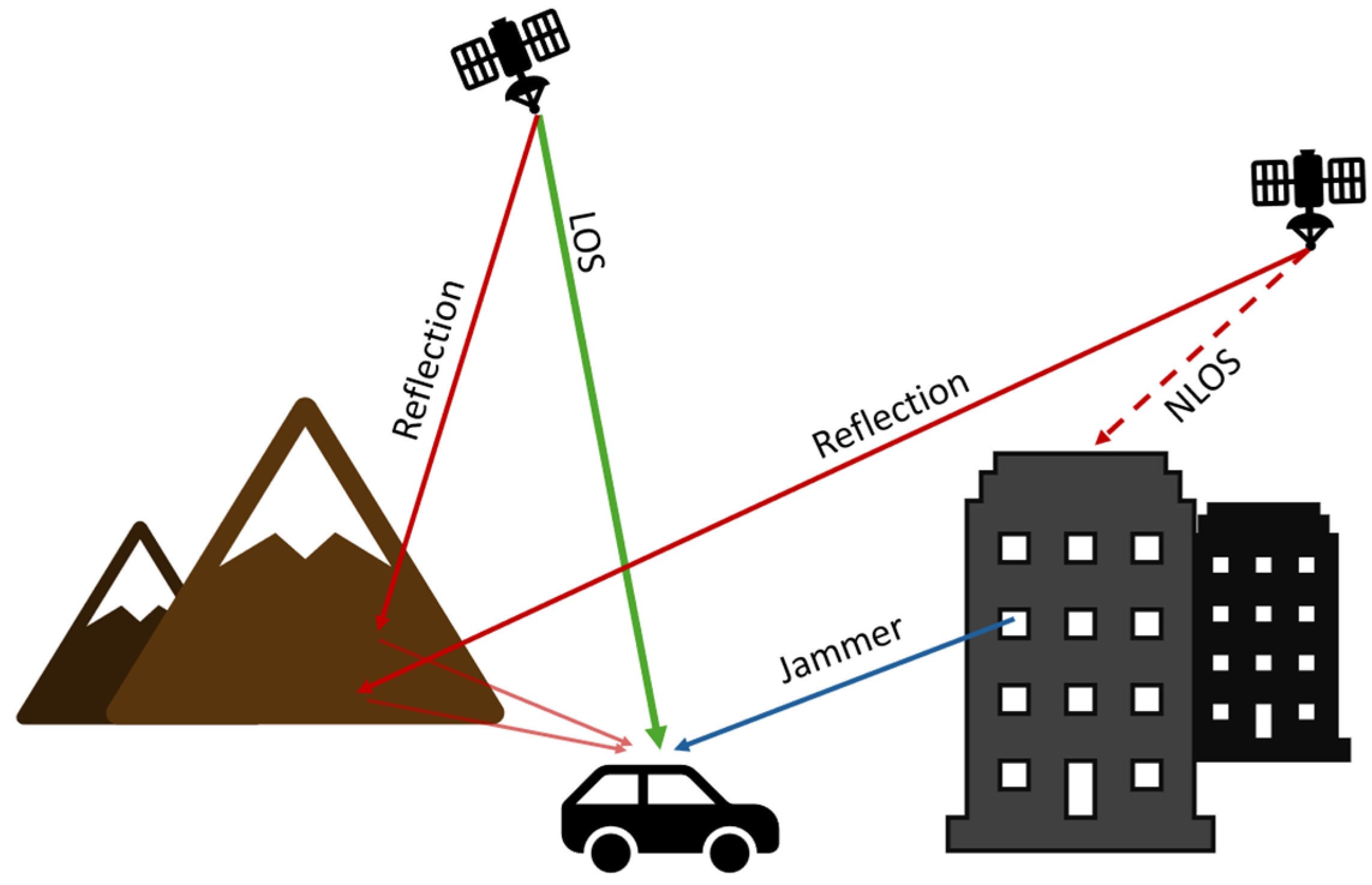
Satellite signals come predominantly from above the antenna (zenith). However, the antenna can also receive multipath signals coming from high- or low-elevation angles, as illustrated in
Figure 1. These are due to signals reflecting on the ground, on buildings, or on geological formations. Additionally, man-made interferences such as jammers can also be present. Jamming signals typically come from low-elevation angles [
6].
Choke ring antennas have concentric conductive walls that reflect signals coming from low-elevation angles, thus reducing the antenna gain in those directions. They have been proposed as solutions to effectively attenuate the unwanted interfering signals [
7,
8]. However, these antennas are static and cannot adapt to a highly dynamic environment such as the ones where autonomous vehicles will need to operate. Additionally, suppose the interferences come from higher elevation angles (such as the top of a tall building or multipath signals in an urban canyon). In this case, the efficacy of the choke ring antenna on ignoring these signals is compromised.
With the use of an antenna array, it is possible to dynamically adjust the radiation characteristics of the antenna, allowing for spatial filtering of the received GNSS signals by attenuating the multipath signals and increasing the gain of direct satellite signals [
9]. Furthermore, it is also possible to identify the Direction of Arrival (DoA) of jamming or spoofing signals and dynamically mitigate them through spatial filtering [
5].
The implementation of an antenna array is not, however, a straightforward task. The increased number of antennas that compose the array occupies a large area and requires a complex feeding network. A beamforming mechanism is also necessary. An analog beamformer uses phase shifters and variable gain amplifiers to control the phase and amplitude of the signals. At least one of each is required for each antenna element that composes the array, leading to complex and expensive setups for large arrays. Digital beamforming is achieved by sampling the incident RF signal at each antenna element using analog-to-digital converters (ADCs), allowing for the reduction in component count and providing greater control over the phase delay between feedlines, at the expense of higher computation cost [
10]. However, every antenna must be directly connected to an ADC, which must be able to sample synchronized signals at a high sampling frequency, requiring ADCs that are usually expensive, making the overall system costly and complex [
11]. Other beamforming techniques, such as Direct Digital Synthesizer and Phase Lock Loop (DDS-PLL), are also available. In DDS-PLL, the signal of each antenna is downconverted twice, with two mixers that use synchronized local oscillators (LOs). By varying the phase of the second LO relatively to the first LO, that same phase shift is induced in the output of the second mixer [
12].
The use of antenna arrays for GNSS multipath and interference mitigation has been attempted and reported in literature, with the solution based on four-antenna planar arrays being the most prominent design reported. In [
13], the authors use a 2 × 2 planar array composed of E1/E5 dual-band patch antennas placed just under λ
0/2 from each other to demonstrate the mitigation of jamming and spoofing signals in realistic scenarios with good results. Similarly, in [
14], a 190 × 190 mm 2 × 2 planar array composed of commercial off-the-shelf (COTS) patch antennas at λ
0/2 spacing was used as part of a system for multipath detection. Resorting to a software-defined radio (SDR), the MUSIC algorithm was implemented and, with beamforming, an increase in C/N
0 of up to 8 dB was achieved. In [
15], a four-element half-wavelength circular array was used in combination with a COTS GNSS receiver and an FPGA to evaluate nulling capabilities for intentional interference mitigation. A field test demonstrated that up to two sources of interference could be countered while maintaining a sufficient carrier-to-noise ratio for the GNSS receiver. In [
16] a 140 × 140 mm
2 planar 2 × 2 array of patch antennas with d = λ
0/3 was presented. Different designs can also be found, with a 1 × 4 linear array of custom-made patch antennas being presented in [
17]. Each patch is 40.9 × 40.9 mm
2 (0.21λ
0 × 0.21λ
0), and the center-to-center distance in the array is 66 mm, around 0.35λ
0 at 1.57542 GHz. The array was controlled by a hardware beamformer, and its beamforming was demonstrated. Being a linear array, the beamforming capabilities were limited from design, and mutual coupling compensation was not considered, which was a considerable design flaw given the close distance between antenna elements in the array. In [
18] a circular array of seven dual-band (L1/L2) antennas was reported. The array had a diameter of 500 mm, and the antennas were spaced by 125 mm. The array was tested for its nulling capabilities with both hardware and software beamforming systems.
However, N-antenna systems can perform nulling operations on N-1 interferences. With the commonly seen four-antenna system, this means filtering three interferences. As such, arrays with more antenna elements may be necessary to optimize the performance of GNSS receivers in complex environments like urban canyons, where multiple interferences may be present (multipath and man-made). The reported arrays are mostly composed of four antennas, since the complexity of the hardware and software required for more antennas will increase rapidly with the number of antennas. The cost is greater due to more components, not only antennas but also ADCs, amplifiers, and filters. For an increase in beamsteering capabilities, the antennas must be maintained at a certain distance from each other, also increasing volume and substrate material demands.
To the best of our knowledge, no GNSS 16-element systems have been documented in the available literature. Commercial solutions do exist, such as the Tualcom TUALAJ 16300—a 16-element Controlled Reception Pattern Antenna (CRPA). This system is capable of suppressing interference from up to 15 jamming sources, effectively generating 15 nulls across three distinct frequency bands.
To improve upon the reported system’s capabilities, in this work, we present a 16 antenna (4 × 4 planar array) solution developed resorting to a powerful FPGA-based array and beamforming development platform (ABDP), designed to expedite the development of arrays and beamforming algorithms [
19]. This approach leverages an innovative reconfigurable platform that supports the testing of any antenna array with up to 16 feeds and an unlimited number of algorithms without requiring major reconfiguration. It can also directly interface with conventional single-antenna receivers and RF test equipment. By modifying only the software layer, there is no need to develop new hardware between design iterations or across different systems. This significantly accelerates the development of complex antenna arrays and beamforming algorithms by eliminating the need to redesign the hardware layer, enabling faster progression toward dedicated solutions for industrial applications.
At this stage of development, a commercial off-the-shelf (COTS) antenna element was used to operate in the L1/E1 band (1.57542 GHz). The array must be designed to be integrated into a car’s rooftop without significantly changing its appearance; therefore, the system must have a small footprint and be as thin as possible. Additionally, the system must be compatible with standard GNSS receivers; therefore, its output signal must be compatible with what is expected from a single antenna that is fed to the receiver for correlation and tracking. The performance will be evaluated under interference constraints while directing the main beam to different directions and evaluating the system’s capabilities to perform multibeam beamforming to track multiple satellites simultaneously. The precise effect of the rooftop’s metal frame on the array’s performance is not under the scope of this paper.
Section 2 presents the design and simulation of the antenna array for GNSS applications.
Section 3 describes the beamforming mechanism [
19] employed in the ABDP and implemented in the ZCU 216 FPGA.
Section 4 presents the integration of the array and the ABDP, along with the full system’s performance evaluation in an anechoic chamber. Finally,
Section 5 discusses the conclusions of this work.
2. Antenna Array Design
To build the antenna array, we start by analyzing the performance of a COTS antenna. The ceramic antenna is a low-cost, low-form-factor passive patch antenna commercialized for GNSS applications. Owing to these attributes, along with its performance, the adequate datasheet, and 3D models that the manufacturer provides for this antenna, it was selected as the commercial antenna to consider for the design of the array. Simulations are performed with full-wave solver Computer Simulation Technology (CST) studio suite 2023 by Simulia.
2.1. Modeling of COTS GNSS Antenna
The first step after picking the antenna was to draw the antenna in CST using both the 3D CAD model and the technical drawing available online. The antenna is composed of five main structures (
Figure 2). The antenna’s position in the ground plane was chosen to be the best location specified in the datasheet by the manufacturer and corresponds to the center of the 70 × 70 × 1.5 mm
3 ground plane. To simulate real testing, a coaxial connector was also added, and the feed port was placed at the end of the connector. The Z-axis of the coordinate system (θ = 0°) is perpendicular to the patch’s surface. The dimensions and materials available in the datasheet/CAD were used.
Table 1 summarizes the antenna parameters, their values, and assigned CST materials.
In the case of the dielectric, the manufacturer only specifies that it is a ceramic. Therefore, a sweep of the dielectric constant, ε
r, was performed to match both the S
11 and axial ratio presented in the datasheet.
Figure 3 shows the results obtained with ε
r = 20.65, which agree with the results in the antenna’s datasheet [
20]. Therefore, this was the value adopted for the antenna array simulations.
The axial ratios (ARs) at 1.57542 GHz in the elevation plane for φ = 0° and φ = 90° are presented in
Figure 4. In both planes, the axial ratio is slightly above 3 dB, the desired axial ratio upper limit for circular polarized antennas on the radiating side of the patch. Although, from
Figure 3, the AR is shown to be below 3 dB, which is only marginally around the frequency of 1.57 GHz, and not at 1.57542 GHz. Note that these results were obtained from the approximated value of ε
r, meaning that they can be slightly off from the actual values.
In
Figure 5, the simulated realized gain patterns for LHCP and RHCP are presented in both φ = 0° and φ = 90° directions. In both directions, the maximum realized gain is −2.95 dBi for LHCP signals (−8.9 dBi if we consider only the top side of the patch). As for the RHCP, the maximum realized gain is 5.15 dBi, which agrees with the datasheet’s stated 5.5 dBi gain. Once again, this behavior shows the RHCP affinity of the antenna.
Finally, the antenna’s apparent phase center was estimated to be at (0.22, 1.70, 1.32) mm, very close to the geometric center of the antenna, which is the reference point (0, 0, 0). To understand the phase center variation, the plots for both the φ = 0° and φ = 90° elevation plane phase for LHCP and RHCP are presented in
Figure 6. In the case of RHCP, in the plane φ = 0°, the phase varies 5.23°, and in the plane φ = 90° it varies 0.68°, for θ between −90° and 90°. These results show that the antenna has a small phase center variation (PCV).
This antenna showed good performance in most of its characterized parameters. The antenna can mitigate LHCP with low gains when compared to RHCP signals and even has low variation in the phase center, which is important for GNSS applications.
2.2. Array Geometry
In this section, the geometry of the antenna array will be discussed, where three key deign parameters were considered: first, the gain and half power beam width (HPBW) of the array, which changes proportionally with the number of antennas; second, the complexity of a future analog or digital beamforming system, as the number of required components, computational power, and cost also increases with the number of antennas in the array; third, the size of the array increases as more antennas are used. With this in mind, a 16-antenna square array was proposed, as it is a good compromise of the three previous figures, along with the square being the most common array geometry.
The distance between elements was chosen to keep the array as small as possible, keeping in mind the limited space availability in the car, without significantly hindering performance, and considering the effect of mutual coupling. For all the accounted combinations of element spacing and array geometry that use 16 antennas, the array factor (AF) was analyzed for broadside, endfire, and in-between configurations using Matlab’ s (version 2022b) Sensor Array Analyzer toolbox.
Since the objective of the work was the development of an antenna array for GNSS signal spatial filtering, high directivity of the AF and low HPBW must be achieved. Analyzing the data concerning square arrays with different element spacing of 0.33λ
0, 0.4λ
0, 0.5λ
0, and 0.75λ
0, it was possible to verify that, as expected, the main lobe directivity increases as the distance d between the array elements increases. On the other hand, the half power beamwidth decreases. Given this, it would seem intuitive that since the goal is to obtain high directivity and low HPBW, d should be as high as possible. However, higher
values lead to more and higher grating lobes: as detailed in [
21] side lobes are small compared to the main beam when the following criteria are met:
Because the intention is to direct the main beam to values of θ ranging from 0° to 90°, from horizon to zenith, ideally
should be less than
to reduce the side lobe level (SLL), coinciding with the following statement from Balanis [
22]: “to have only one end-fire maximum and to avoid any grating lobes, the maximum spacing between elements should be less than
”.
A compromise between the directivity and HPBW of the array with d = 0.5λ
0 and the low grating lobe level achieved with d = 0.33λ
0 is achieved with d = 0.4λ
0.
Figure 7 shows why an element spacing of d = 0.5λ
0 is not ideal due to having two main beams in opposite directions at θ = 90° compared to a spacing of d = 0.4λ
0. It is also presenting the radiation pattern for θ = 0°, where the directivity difference, the HPBW, and the reducing of side lobe levels are noticeable, as mentioned above.
2.3. Array Simulation
The antenna array was designed in CST resorting to the Array Task tool and it was studied with its main beam pointing towards the following set of φ and θ angles: (0,0), (0, 45), (0,90), (45, 45), (45, 90), (90, 45), and (90, 90). This selection of directions allows for the study of the array’s characteristics and performance when pointing to the zenith (broadside) and to the horizon (endfire) in two orthogonal planes and with a step in-between. As the antennas in the array are symmetrically positioned, the performance in this 90° segment of the array is representative of the array’s performance in the remaining directions.
The 3D model of the square array of d = 0.4λ
0 and size of 305 × 305 mm
2 is presented in
Figure 8. The ground plane of each antenna element was extended so it is a single structure common to all antennas.
The simulated 3D radiation patterns of the square array pointing to the previously enumerated directions are presented in
Figure 9, and the 2D plots in the elevation plane cut are presented in
Figure 10. As can be seen, the gain is highest in the broadside direction (14.9 dBi), as expected, since both the antenna element gain and the array factor’s directivity are highest in this direction. When θ = 45°, the gain is slightly lower (13.3 dBi for φ = 0°), as both the antenna element gain and the array factor directivity are lower at this angle. This fact is also the reason why the array is not capable of adequately pointing the beam towards θ = 90°: The antenna element has much lower gain towards the horizon, thus hindering the array’s performance in this plane. However, the array is still capable of achieving a gain of 6.2 dBi for φ = 0° and θ = 90° and 5.2 dB for φ = 90° and θ = 90° while the single-antenna element can only provide a gain of −3.4 dBi and −3.0 dBi, respectively, thus accomplishing the goal of improving signal reception at low elevations.
Figure 11 presents the axial ratio of the array when the main beam is directed towards the aforementioned directions. It is possible to observe that the array maintains reasonable circular polarization (AR close to 3 dB) in the directions the main beam points to. This statement holds even for beam directions of θ = 90°, except for the case where φ = 0°, where the AR at the 90° mark is over 10 dB. This could be due to the inherent asymmetry of the antenna element on the square array, and it is a possible path to be explored in future work.
3. Beamforming System
Beamformers can be divided into their analog and digital counterparts [
23,
24]. Analog beamformers modify phase and gain through phase shifters and variable gain amplifiers, while digital beamformers change them by multiplying the sampled signals by complex weights. However, the control platform used is very similar for both. Both require a control platform used to calculate the phases or complex weights usually using very similar algorithms. In this work, we employed the ABDP platform [
19] to test digital beamforming approaches resorting to a Zynq UltraScale+ RFSoC ZCU216 evaluation board from Xilinx, which utilizes the XCZU49DR RFSoC. The objective of implementing this architecture is to expedite the development of arrays and beamforming algorithms through the design, iteration, test, and validation stages. This is achieved by providing a software-defined system that can test a multitude of configurations (array size, geometry, number of elements, frequency, etc.) and beamforming algorithms (classic and adaptive) without requiring hardware modifications. We believe that this will ultimately drive the cost of final products down by reducing development time and cost.
The block diagram of the proposed system is presented in
Figure 12, and it is composed of four major components: the ADCs, the processing system (which includes the beamforming algorithm), the programmable logic, and the DAC.
The digital samples from each antenna’s signal acquired by the ADCs are supplied to the programmable logic (PL) via the PL interface, where weights calculated by the beamforming algorithm are applied to the samples. The output of the PL contains the improved signal containing information of every satellite. Before converting the signal back to its analog form, the signal must be modulated back to the 1.57542 GHz frequency. The result is a similar signal to the one sampled, but now with improved satellite signal quality. It can then be converted to its analog form using the DAC. This analog output can then be supplied to a traditional GNSS receiver.
The calibration process for the different channels and the applied compensations to guarantee phase balance and group delay are detailed in [
19], along with a detailed description and validation. Furthermore, the configuration of the FPGA’s parameters such as sampling rate are also presented in [
19].
4. Measurement Results and Performance Analysis
The antenna array was integrated into the ABDP for testing of the full system in an anechoic chamber. Each of the antennas was connected to one of the 16 ADC channels of the ZCU216 board, and the system was placed in the anechoic chamber as demonstrated in
Figure 14. The antenna array was mounted on a foam platform facing the transmission antenna (WBH2-18S from Q-Par Angus, Leominster, UK) and the ABDP covered in panels that absorb RF waves. Additionally, the DAC to which the output of the beamforming is being routed to, was connected to PORT2 of the Vector Network Analyzer (VNA).
The azimuth plane radiation patterns of the array were first obtained for four directions at two different planes. The planes tested were φ = 0°and φ = 45 °, where the main beam was pointed towards θ = 0° (broadside), θ = 340°, θ = 45°, and θ = 300°. The same radiation pattern was simulated in CST, and the results are presented in
Figure 15 and
Figure 16.
There is a great agreement between the measured and simulated patterns. In terms of the main lobes, it was possible to point the beam at the desired positions, with a noticeable deviation at higher θ values, such as in the θ = 60° and θ = 300°, which was expected as discussed previously. Nevertheless, the measurements and the simulations present the same limitations of the system. There is a slight difference in the side lobes and the nulls between the two planes. In the φ = 45° plane, there is a slightly larger null and side lobe relative to the simulations. This can be due to mutual coupling between antenna elements that is not reproduced by the simulations, due to material imperfections, or small misalignments in the measurement setup and the array itself. It is not possible to compare the absolute gain values of the measurement with the simulation because the analog signal measured by the VNA is generated by the DAC of the ZCU216, as previously discussed. Moreover, these results are normalized to the value at φ = 0° and θ = 0°, separately for the two planes.
In addition to the single-beam tests, a multibeam radiation pattern was also simulated and measured. The three beams were pointed towards θ = 0°, θ = 45°, and θ = 330°. The azimuth plane radiation patterns are presented in
Figure 17. It is possible to observe that the proposed system successfully produced a radiation pattern with the three proposed beams. The measured multibeam radiation pattern greatly matches the predicted one. As can be seen, the maxima were pointed towards the desired θ = 0° and θ = 45° directions, while the beam towards θ = 330° was slightly shifted towards θ = 315°. Since this was predicted by the simulation, it is possible to conclude that this was due to the array’s resolution limitation. This could potentially be improved with the use of arrays with more elements. In the direction of θ = 330°, it is noticeable that the measured gain deviates slightly from the theoretical value. This can be explained by the measurement setup demonstrated in
Figure 14. When pointing towards θ = 330°, the array starts to turn towards the box containing the ABDP and the cables, which interferes with the ideally anechoic environment of the anechoic chamber, leading to a reduction in the received power.
Thanks to the use of 16 array elements, the radiation pattern performance of this system is superior compared to some of the above referenced papers using beamforming for GNSS systems. For example, in [
14], a 2 × 2 antenna array is implemented using SDR software, MUSIC. This antenna array achieves a maximum gain of approximately 11 dBi, a half-power beamwidth (HPBW) of 60°, an SLL of less than 9 dB when the main beam is steered to 30°, and a first-null-to-peak difference of 17 dB. In contrast, the proposed 16-element array achieves a significantly higher maximum gain of 14.9 dBi, a narrower HPBW of 30°, an SLL of 15 dB when the beam is pointed at boresight, and a first-null-to-peak difference exceeding 35 dB.
5. Conclusions and Future Work
In this work, a GNSS adaptive antenna array with digital beamforming was reported. The array was developed with COTS GNSS antennas. The performance of these antennas was validated via simulation in CST. The array geometry was studied resorting to Matlab, and the final array simulations were performed in CST. It was demonstrated that the proposed array can improve the gain comparatively to the traditional GNSS antenna in all directions, even close to the horizon. It was also possible to observe that the array maintains reasonable circular polarization in the directions to which the main beam points.
A digital beamforming solution was developed in Xilinx’s ZCU216, with each of the array’s 16 antennas being connected to an ADC channel. The GNSS signals, after being sampled by the ADCs, were weighed according to a beamforming algorithm that received as inputs the direction towards which the main beam was to be pointed. The full system was tested in an anechoic chamber, where good results were obtained in both single- and multibeam scenarios, with a great agreement between the simulated and measured data.
Nevertheless, desirable improvements in the system have been identified, namely the use of custom GNSS antennas with better AR over the range of interest. Furthermore, it was verified that in the multibeam approach, the results could be improved by developing an array with an improved HPBW, either by using more directive antenna elements or by geometry redesign.
The results presented in this paper validate the FPGA-based array and beamforming development platform, paving the way for the seamless and rapid design and test of numerous antenna array geometries with up to 16 channels and beamforming algorithms, including adaptive ones. This powerful and versatile tool will accelerate research on the performance improvement of GNSS reception.


