Fault Detection for Power Batteries Using a Generative Adversarial Network with a Convolutional Long Short-Term Memory (GAN-CNN-LSTM) Hybrid Model

Abstract

With the rapid proliferation of new energy vehicles, the safety of power batteries has attracted increasing attention. As a crucial approach to ensuring system stability, fault detection has become a research focus. However, strong temporal dependencies in battery operation data and the scarcity of fault samples hinder the accuracy and robustness of existing methods. To address these challenges, this paper proposes a deep learning-based fault detection model that integrates a Generative Adversarial Network (GAN) with a Convolutional Long Short-Term Memory (CNN-LSTM) network. The GAN is employed to augment minority-class fault samples, effectively mitigating the class imbalance in the dataset. Then, the CNN-LSTM module directly processes raw multivariate time-series data, combining the capability of CNN in extracting local spatial patterns with the LSTM strength in modeling temporal dependencies, enabling accurate identification of battery faults. Experiments conducted on real-world datasets collected from electric vehicles demonstrate that the proposed model achieves a Precision of 95.23%, Recall of 87.23%, and F1-Score of 91.12% for fault detection. Additionally, it yields an Average Precision (AP) of 97.45% and an Area Under the ROC Curve (AUC) of 99%, significantly outperforming conventional deep learning and machine learning baselines. This study provides a practical and high-performance solution for fault detection in power battery systems, with promising application potential.

1. Introduction

Among various power battery technologies, lithium-ion batteries have emerged as the mainstream choice for new energy vehicles due to their high energy density, long cycle life, and excellent environmental adaptability. In particular, ternary lithium batteries and lithium iron phosphate batteries are widely adopted in both battery electric vehicles (BEVs) and hybrid electric vehicles (HEVs), serving as core components to replace traditional fossil fuel systems [1]. With the advent of the intelligent driving era, the increasing demand for high-performance onboard chips, sensors, and communication equipment imposes higher requirements on the performance and stability of power supply systems. As a key energy source, the safety of power batteries is directly linked to vehicle stability and passenger safety.

However, the rapid increase in the number of new energy vehicles has brought growing concerns over battery-related safety incidents. In real-world operations, power batteries are prone to various types of faults, such as thermal runaway, lithium plating, and electrolyte leakage. These failures are often triggered by internal short circuits, overcharging, or casing damage, potentially leading to severe consequences including fires and explosions [2]. In major markets like China and the United States, battery incidents are frequently reported by government agencies and media. Since 2019, over 600 power battery-related fires have been documented in cities like New York and San Francisco alone. According to China’s Ministry of Emergency Management, more than 3000 EV-induced fire accidents occurred in 2023. Such incidents are characterized by rapid combustion and high destructiveness, leaving very limited escape time for passengers. Consequently, developing efficient battery fault detection mechanisms has become a pressing research focus in both academia and industry [3].

Current battery fault detection methods can be broadly classified into two categories: (1) physics-based approaches, which rely on thermodynamic, electrochemical, or control models to analyze battery status; and (2) data-driven approaches, which use machine learning or deep learning techniques to model and classify battery behaviors from collected data [4]. Compared with traditional methods, data-driven approaches offer automated modeling capabilities without requiring complex physical assumptions, and they exhibit stronger adaptability when handling complex, non-linear, and multivariate data. Nevertheless, two key challenges remain: first, battery operation data exhibit strong temporal dependencies, and effectively modeling these time-series correlations is critical [5]; second, fault samples are rare, resulting in highly imbalanced datasets that hinder the model’s ability to learn fault patterns, thus degrading detection performance [6].

To address the above challenges, this paper proposes a deep learning-based fault detection framework that integrates a Generative Adversarial Network (GAN) with a Convolutional Long Short-Term Memory (CNN-LSTM) network. The main contributions of this work are as follows:

1.

A GAN-based sample generation method is developed to synthesize time-consistent pseudo-fault samples by learning the distribution of real fault data, effectively alleviating class imbalance.

2.

A hybrid CNN-LSTM classification model is designed to extract both spatial and temporal features from raw battery time-series data, enabling accurate modeling of time dependencies while preserving local structures.

3.

Extensive experiments on real-world power battery charging datasets are conducted, and comparisons with traditional machine learning and various deep learning models demonstrate the proposed method’s superiority in terms of detection accuracy, robustness, and generalization performance.

2. Related Work

2.1. Overview of Fault Detection Methods for Power Batteries

Currently, fault detection methods for power batteries can be broadly categorized into two types: model-based approaches (also referred to as traditional methods) and data-driven approaches. The former relies on thermodynamic, electrochemical, and control models to provide interpretable mathematical formulations for monitoring and predicting fault conditions. In contrast, the latter leverages machine learning or deep learning techniques to learn patterns of state evolution from large volumes of battery operation data, enabling intelligent fault diagnosis and early warning.

Model-based approaches typically monitor key parameters such as voltage, current, and temperature, and trigger alarm signals through the Battery Management System (BMS) when any measurement exceeds preset thresholds [7]. Berecibar et al. provided a comprehensive review of equivalent circuit models (ECMs) and electrochemical models used in BMSs, highlighting their roles in thermal management and overcharge protection [8]. Sun et al. proposed an internal short-circuit detection method based on residual voltage, capable of identifying latent faults under real driving conditions [9]. Although these approaches can achieve high accuracy under ideal or well-defined conditions, they are heavily dependent on model parameters and often struggle to adapt to non-linear battery behaviors, aging effects, and variable operating conditions.

In contrast, data-driven methods have gained increasing attention in recent years due to their strong capability in capturing complex patterns. These methods learn the distributions of fault and normal conditions from historical battery data and build classifiers for fault detection [10]. Zhang S et al. reviewed the applications of traditional machine learning techniques such as Support Vector Machines (SVMs), decision trees, and random forests in battery health evaluation, noting their good generalization performance in low-dimensional scenarios [11]. With the rise of deep learning, researchers have explored using convolutional neural networks (CNNs) and recurrent neural networks (RNNs) for battery fault diagnosis [12]. Zou et al. integrated incremental capacity analysis (ICA) with CNNs to develop a deep feature-driven early fault detection method that significantly improved classification performance [13]. Arévalo and Zhang Y, from a model perspective, systematically reviewed the applications of artificial intelligence in BMSs, and highlighted the importance of LSTM networks, autoencoders, and reinforcement learning in life prediction and state monitoring [14,15]. Zhao et al. constructed a deep neural network framework based on incremental voltage topology to efficiently identify multiple types of battery faults [16]. Zheng et al. improved detection accuracy by combining segmented regression with gated recurrent units (GRUs) [17], while Liu et al. proposed a hybrid algorithm based on symmetric deviation point (SDP) patterns and CNNs to detect typical failures such as overcharging, over-discharging, aging, and leakage [18].

In summary, model-based approaches provide strong interpretability and theoretical grounding and are well-suited to scenarios with well-understood mechanisms and clearly defined structures. However, their performance is limited when dealing with real-world conditions involving multivariate coupling, non-linear dynamics, and complex operating environments. Data-driven methods, while more sensitive to data quality and model selection, offer greater flexibility, adaptability, and predictive accuracy in modeling non-linear relationships and identifying complex features, thus demonstrating superior robustness and practical value in power battery fault detection.

2.2. Overview of Imbalanced Data Handling Methods

The class imbalance problem is prevalent across many domains, including fault detection, medical diagnosis, financial fraud detection, and natural language processing. When the number of minority class samples is significantly lower than that of the majority class, classification models tend to be biased toward the majority class, leading to poor recognition of critical minority instances and severely degrading overall performance and generalization capability.

To address this issue, researchers have proposed various sample reconstruction strategies, among which undersampling and oversampling are the most common. Undersampling aims to achieve class balance by strategically reducing the number of majority class samples. Batista et al. developed several undersampling algorithms based on clustering and nearest neighbors to improve the classification of minority instances [19]. However, this approach may risk losing valuable information, making it less suitable for high-dimensional and complex tasks.

In contrast, oversampling generates synthetic minority samples to achieve balance without discarding original data, and is therefore more widely adopted. The most representative technique is SMOTE (Synthetic Minority Oversampling Technique), which interpolates between existing minority samples to create new ones, effectively enhancing the model’s ability to learn from minority data. Based on SMOTE, researchers have proposed improved variants such as Borderline-SMOTE and ADASYN, which place greater emphasis on boundary samples and adaptive sample generation, respectively [20,21].

In recent years, with the advancement of deep learning, generative models such as Generative Adversarial Networks (GANs) and Variational Autoencoders (VAEs) have been introduced into imbalanced learning. Mariani et al. combined GAN and VAE to generate high-quality minority class samples, offering a more diverse and realistic data distribution than traditional interpolation-based methods [22]. Other approaches—such as attention mechanisms to enhance focus on critical features, multi-branch network designs, transfer learning, and self-supervised learning—have also been explored to mitigate data imbalance [23].

In the context of power battery fault detection, the minority class typically represents fault data, which are much less abundant than normal operation data. Considering the rarity and difficulty of acquiring fault samples, this study adopts a GAN-based oversampling strategy to balance class distribution while preserving feature integrity, thereby providing a more reliable foundation for classifier training.

2.3. Overview of Multivariate Time-Series Classification Methods

The operation of power batteries in new energy vehicles generates large volumes of data across multiple dimensions, including voltage, current, temperature, internal resistance, and time. These data exhibit strong temporal dependencies and multivariate coupling characteristics, forming a typical multivariate time-series structure. For such complex data, traditional univariate models often fail to effectively capture inter-variable interactions and dynamic patterns, thereby limiting classification performance.

In recent years, deep learning methods have demonstrated significant advantages in modeling multivariate time-series data. Various network architectures have been proposed to jointly extract temporal and spatial features. Originally designed for image processing, convolutional neural networks (CNNs) have proven effective in local pattern extraction and have been adapted for time-series tasks. By treating time-series data as pseudo-image structures and applying one-dimensional convolutions (1D-CNNs) along the temporal axis, CNNs can efficiently capture local dependencies and spatial features [24]. On the other hand, recurrent neural networks (RNNs) are more suitable for handling sequential data with strong temporal correlations. In particular, Long Short-Term Memory (LSTM) networks, with their gated mechanisms that selectively retain or forget past information, excel at capturing long-range dependencies. For instance, Fawaz et al. employed a bidirectional LSTM architecture for multivariate time-series classification tasks such as ECG signal analysis and human activity recognition, achieving notable success in real-world applications [25].

Therefore, in the context of power battery fault detection, the selected deep learning model must be capable of modeling the strong inter-feature coupling, temporal dependencies, and non-linear structure inherent in multivariate time-series data.

Compared with traditional machine learning approaches and existing deep learning methods, our proposed approach addresses class imbalance by employing a GAN to generate minority class samples that better fit the true data distribution, rather than using simple interpolation methods. For the classifier, we adopt a hybrid CNN-LSTM structure, which enables effective extraction of both fine-grained local variations (via CNN) and long-term temporal dependencies (via LSTM) from raw battery time-series data, minimizing information loss while improving classification performance. Experimental results demonstrate that our method consistently outperforms baseline models—including Random Forest, Logistic Regression, and standalone CNN-LSTM—in terms of Precision, Recall, and AUC, showing superior accuracy and robustness.

3. Data and Preprocessing

The dataset used in this study was provided by a new energy vehicle manufacturer. It consists of power battery operation data collected during the charging phase from multiple vehicles of the same model. Notably, the dataset includes several battery samples that were retrospectively confirmed to have experienced faults. These faults were not successfully detected by the conventional Battery Management System (BMS) during actual operation, making the data particularly valuable for research purposes.

The dataset contains a total of 28,389 samples, each represented as a multivariate time series with a shape of (256, 8). This indicates that eight key features are recorded across 256 time steps, namely, voltage, current, State of Charge (SOC), maximum cell voltage, minimum cell voltage, highest cell temperature, lowest cell temperature, and timestamp.

Each sample is associated with a label: a label of 1 indicates that the vehicle subsequently experienced a fault (positive class), while a label of 0 denotes a normal charging process (negative class).

This dataset realistically reflects the battery’s operational status under diverse conditions and includes key samples in which faults went undetected by traditional BMS, providing a solid foundation for evaluating the effectiveness of deep learning methods in early fault diagnosis.

Statistical analysis of the dataset reveals 23,735 normal (negative) samples and 4654 faulty (positive) samples, resulting in a class ratio of approximately 1:5. This pronounced class imbalance may bias classification models toward the majority class during training, impairing their ability to identify the critical minority class (i.e., fault samples). Therefore, to ensure effective learning and reliable fault identification, it is necessary to introduce appropriate data balancing strategies to mitigate the adverse effects of class imbalance.

Subsequently, a data integrity check was performed on the raw dataset, and no missing values or formatting errors were detected. To eliminate the influence of differing physical scales among features, Z-score normalization was applied to all variables, enhancing feature comparability and accelerating model convergence.

Given that power battery data represent a type of multivariate time series, analyzing the correlations among features is crucial for effective modeling. In this study, correlation analysis was conducted from two perspectives:

(1)

intra-sample feature relationships, and

(2)

statistical correlations across the entire dataset.

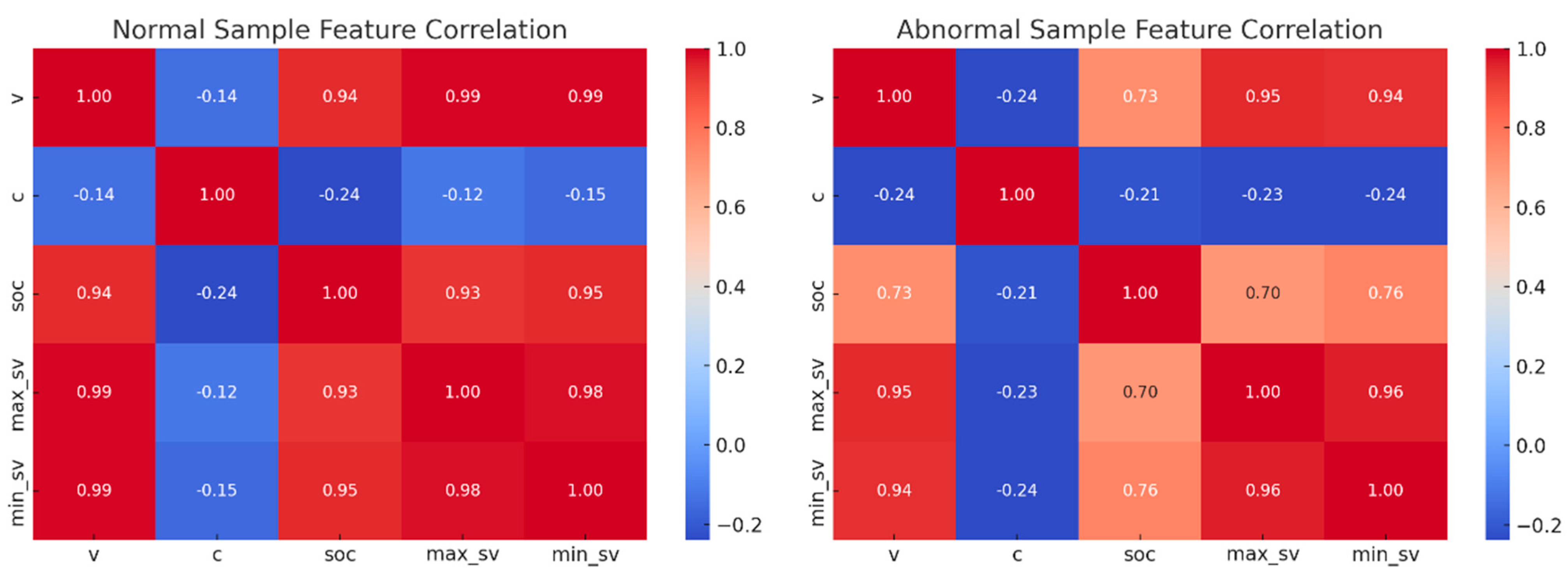
For intra-sample analysis, we selected one normal sample and one faulty sample and calculated the Pearson correlation coefficients among the eight time-series variables. As shown in Figure 1, both samples exhibit strong correlations among most features (such as voltage, current, and SOC), except for maximum/minimum cell temperature and timestamp.

A closer inspection reveals differences in the correlation coefficients between the selected normal and faulty samples, for example, the correlation between current and SOC has changed, suggesting that faults may alter the inter-feature relationships in the battery data.

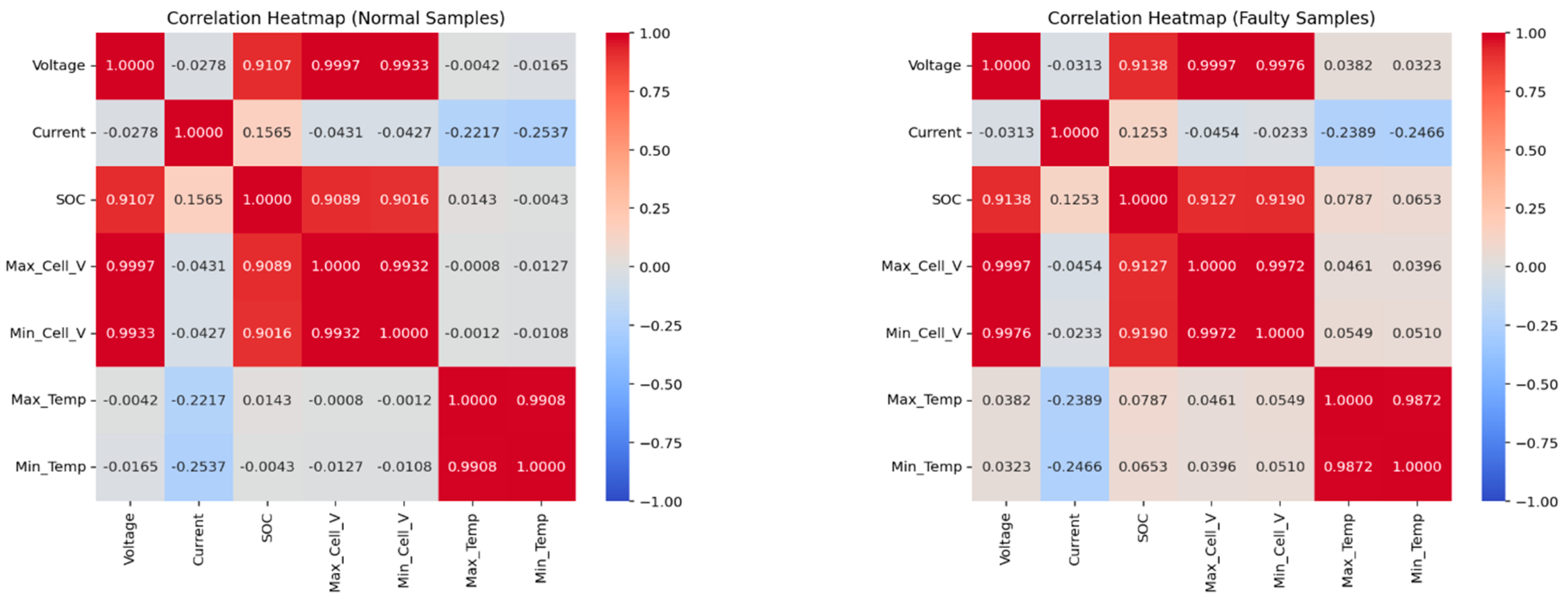
To further examine whether battery faults lead to changes in inter-feature relationships, we computed the pairwise correlation coefficients for all features across the full sets of normal and faulty samples. The resulting correlation heatmaps, shown in Figure 2, reveal observable differences between the two groups, although most changes are relatively small in magnitude. We also performed statistical significance testing using the Fisher r-to-z transformation, and the results indicate that all feature pairs exhibit statistically significant differences in correlation coefficients between normal and faulty samples (p < 0.001).

This finding suggests that battery faults induce subtle but detectable structural changes in feature relationships. Therefore, it is essential for subsequent classification models to be sensitive enough to capture these minor shifts in data characteristics, which could enhance fault detection performance.

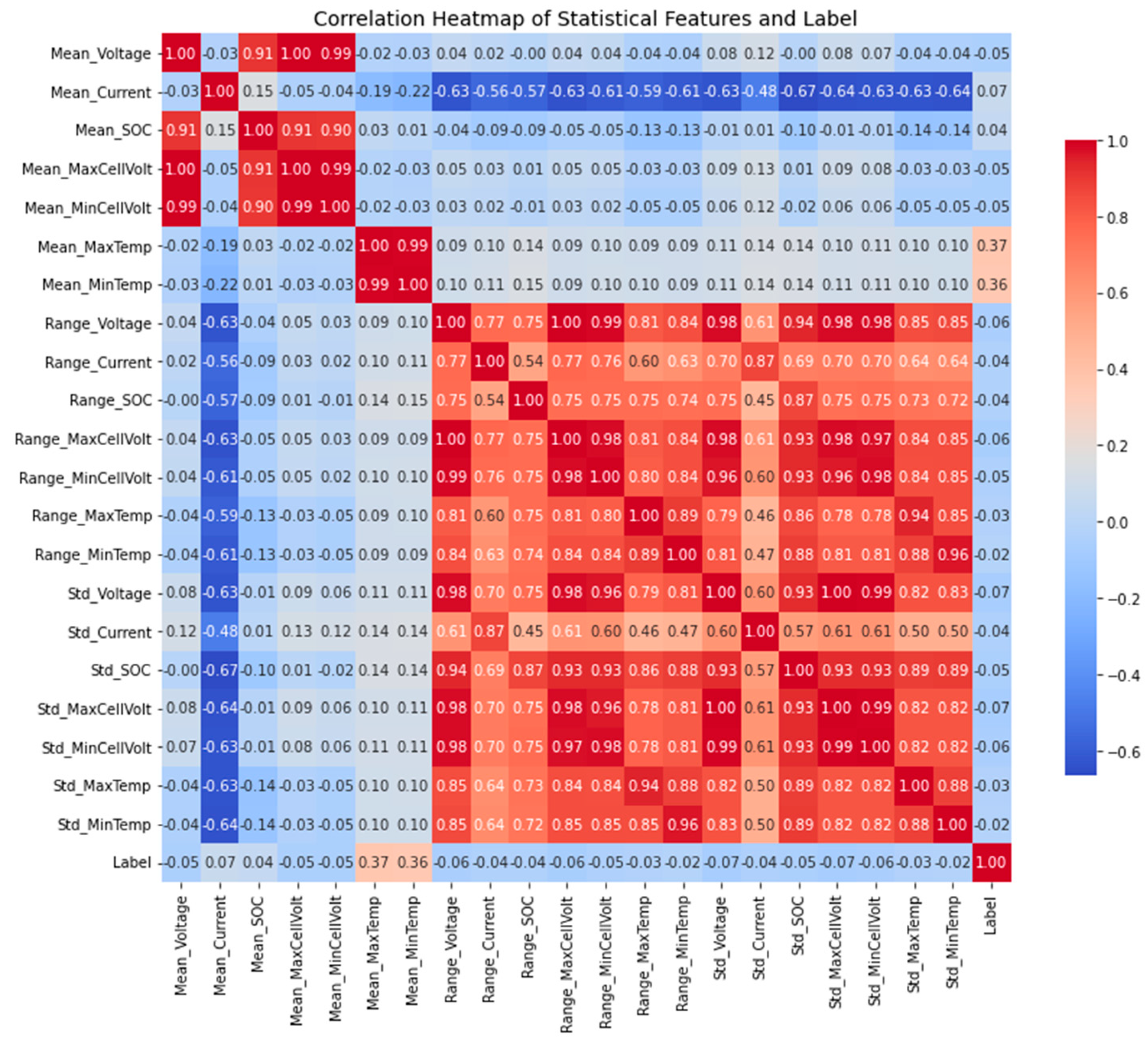
At the full-dataset level, we extracted statistical features from each sample sequence, including mean, range, and standard deviation for each of the seven measurable variables (excluding the non-comparable timestamp). This process compressed the original sample dimension from (28,389, 256, 7) to (28,389, 21). Subsequently, sample labels were incorporated into the correlation analysis, and a Pearson correlation heatmap was generated to illustrate global feature-label relationships, as shown in Figure 3.

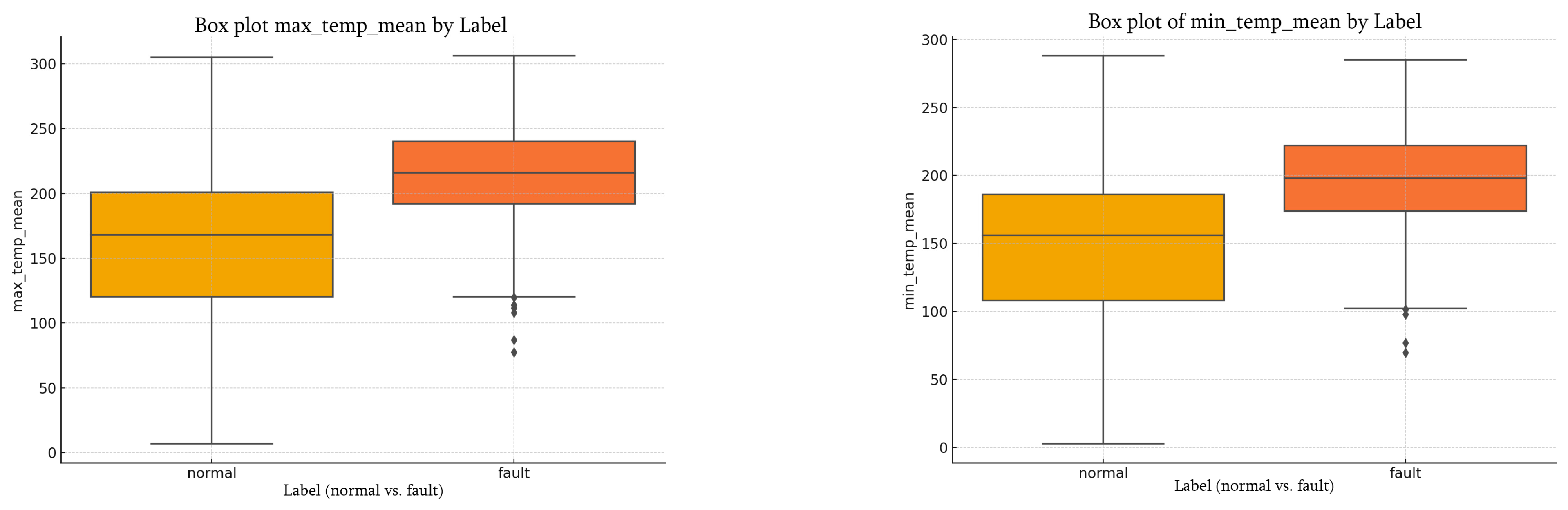
The results indicate that many features in the battery operation data exhibit varying degrees of correlation with the fault label. For instance, as shown in Figure 4, the mean values of maximum and minimum cell temperatures in faulty samples are generally higher than those in normal samples, potentially reflecting risks of thermal runaway or overheating. To confirm the statistical significance of these differences, independent two-sample t-tests and Mann–Whitney U tests were performed on the per-sample mean values, yielding p-values less than 0.001, thus indicating a highly significant difference.

Overall, the correlation analysis demonstrates that battery faults can lead to subtle changes in intra-sample feature relationships, and, at the population level, all measured features provide useful discriminative information for fault detection. Therefore, in subsequent model development, we retain all original features without dimensionality reduction or feature selection, enabling the deep learning model to capture spatial coupling and weak abnormal signals among multivariate time-series data.

4. Methodology

4.1. Overall Framework

Traditional fault detection methods for power batteries often rely on manually defined threshold rules to identify anomalies. However, such methods struggle to deliver satisfactory performance when faced with the complex, dynamic, and non-linear nature of real-world battery operation. To address these limitations, this study proposes a two-stage hybrid model based on deep learning, aiming to effectively detect faults in power battery operational data.

Power battery data typically exhibit strong time-series characteristics and are subject to severe class imbalance between normal and faulty samples. To tackle these two key challenges, we design a detection framework that integrates a Generative Adversarial Network (GAN) for data augmentation and a Convolutional Long Short-Term Memory (CNN-LSTM) network for sequence modeling and classification.

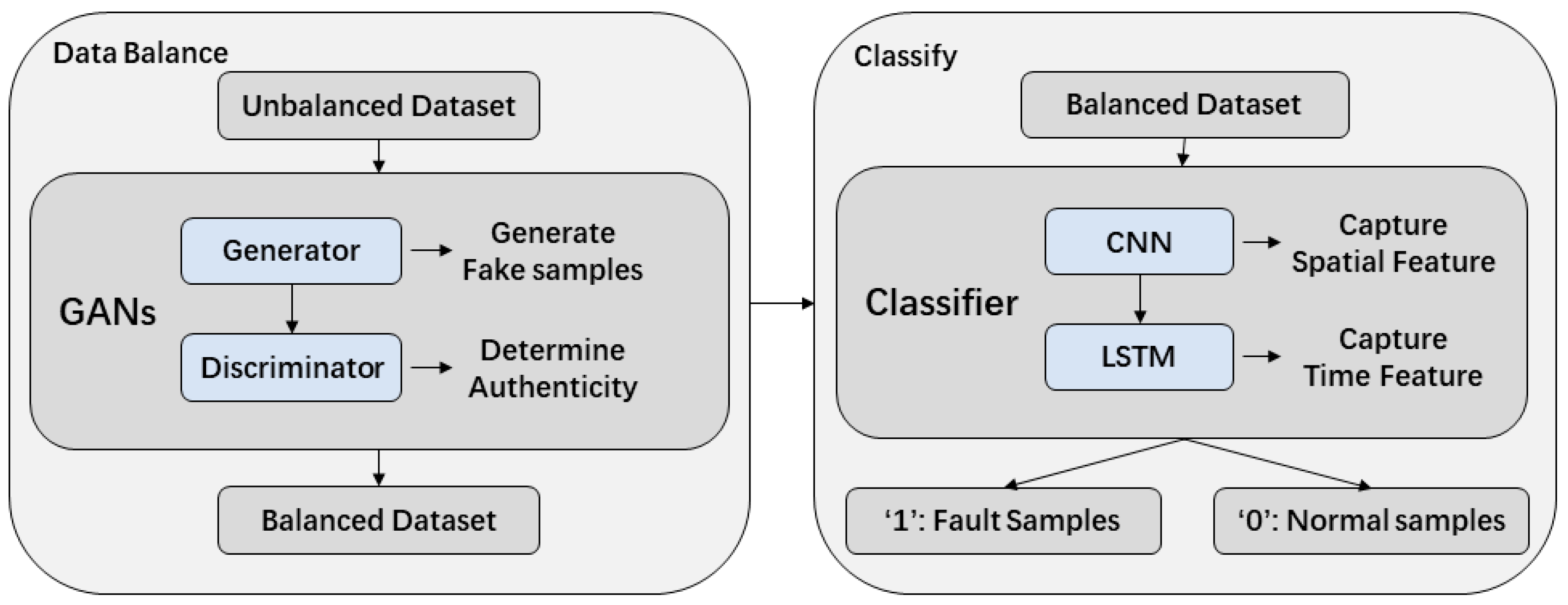
The overall architecture of the proposed model is illustrated in Figure 5.

In the first stage, the GAN module—comprising a generator and a discriminator—operates through adversarial training, where the generator is iteratively optimized to synthesize new samples that closely resemble the distribution of real faulty data. Once trained, the generator is used to augment the minority fault class, producing a balanced dataset in which the number of fault and normal samples is approximately equal.

In the second stage, the CNN-LSTM module is responsible for modeling and classifying the balanced multivariate time-series data. The CNN component extracts local spatial patterns from the battery operation sequences, while the LSTM network captures temporal dependencies and dynamic evolution across time steps. Through this joint architecture, the model achieves accurate identification of battery fault states.

4.2. Generative Adversarial Network (GAN) Module

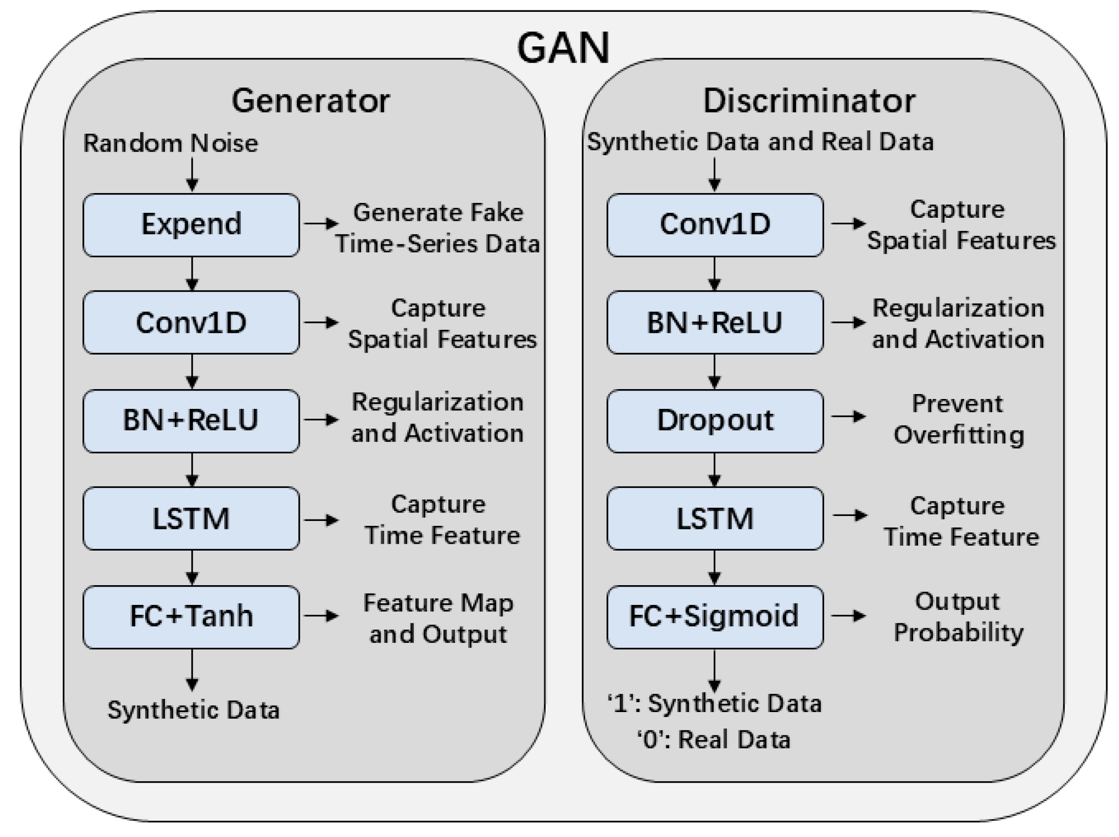
To address the issue of insufficient fault samples and severe class imbalance, this study introduces a Generative Adversarial Network (GAN) to perform data augmentation for the minority class. A GAN consists of a generator and a discriminator, which are optimized through adversarial training to produce synthetic samples that approximate the distribution of real data. The overall architecture is illustrated in Figure 6.

The generator takes a random noise vector as input and outputs synthetic fault samples that match the shape of real charging time-series data. The discriminator receives both real and generated samples and aims to distinguish whether the input comes from the true data distribution. To ensure consistency in data structure, the generator’s output is designed to match the original sample with shape (256, 8).

Specifically, the generator is composed of the following five modules:

• Expand module: Expands the input noise vector into a pseudo time series with shape (256, latent_dim) to simulate the multivariate temporal structure.
• Conv1D module: Applies one-dimensional convolution to extract spatial features from local time windows, enhancing the model’s ability to capture short-term dynamics such as sudden voltage or current fluctuations.
• BN + ReLU module: Uses Batch Normalization to stabilize training and ReLU activation to introduce non-linearity.
• LSTM module: Models long-term temporal dependencies and captures trends, lags, and cross-time behaviors throughout the charging process.
• FC + Tanh module: Maps the encoded features to the target output dimension using a fully connected layer, followed by a Tanh activation function to constrain the output within [−1, 1], ensuring consistency with the real sample range.

This generator design effectively captures both local and global features in time-series data, improving the realism of the generated samples. The specific network layer details and parameter settings for each layer of module are shown in

Table 1. Generator network architecture and settings.

Module	Content	Parameter Setting	Output Size (B = Batch Size)
1	Input (Latent Noise)	latent dim = 64	(B, latent_dim)
	Repeat		(B, 256, latent_dim)
	Permute		(B, latent_dim, 256)
2	Conv1D	in channels = 8 kernel = 3 padding = 2 out channels = 64	(B, 64, 256)
3	BatchNorm +ReLU Permute		(B, 64, 256)
			(B, 256, 64)
4	LSTM	input size = 64 hidden = 128	(B, 256, 256)
5	Linear + Tanh	input size = 256 output size = 8	(B, 256, 8)

.

The discriminator shares a similar architecture to the generator and is designed to distinguish whether an input sequence is real or generated. Its network includes the following components:

• Conv1D module: Extracts key features from short time-series segments.
• BN + ReLU module: Regularizes convolution outputs and introduces non-linear representational capacity.
• Dropout module: Randomly disables a portion of neurons during training to mitigate the risk of overfitting.
• LSTM module: Further models long-range dependencies in the input sequences.
• FC + Sigmoid module: Compresses the encoded sequence into a single probability value representing the confidence that the input is real.

This design enhances the discriminator’s ability to capture temporal structures and feature distributions, making it more effective in differentiating real from synthetic data. The specific discriminator’s network layer details and parameter settings for each layer of module are shown in

Table 2. Discriminator network architecture and settings.

Module	Content	Parameter Setting	Output Size (B = Batch Size)
1	Input (Time-series data)	in channels = 8 kernel = 5 padding = 2 out channels = 64	(B, 256, 8)
	Permute		(B, 8, 256)
	Conv1D		(B, 64, 256)
2	BatchNorm + ReLU		(B, 64, 256)
3	Dropout	p = 0.3	(B, 64, 256)
4	Permute	input size = 64 hidden size = 128	(B, 256, 64)
	LSTM		(B, 256, 256)
5	TimeStep Extract Linear Sigmoid	input size = 256 output size = 1	(B, 256)
			(B, 1)
			(B, 1)

.

To generate high-quality synthetic samples, this study employs a standard adversarial training mechanism, where the generator and discriminator are optimized in an alternating fashion. During training, the parameters of both networks are updated independently via backpropagation. In each iteration, the discriminator is first trained using real fault samples to enhance its discrimination ability, encouraging it to assign high confidence scores to real data. Then, with the discriminator’s parameters fixed, the generator receives random noise vectors and produces synthetic samples in an attempt to “fool” the discriminator, i.e., to make it mistakenly classify the fake samples as real.

Throughout this adversarial game, the generator continuously adjusts its parameters to improve the realism of its outputs, while the discriminator is iteratively optimized to strengthen its ability to distinguish between real and fake data. Eventually, a dynamic equilibrium is reached, in which the generator produces samples that closely match the distribution of real data, making it increasingly difficult for the discriminator to accurately identify their origin.

In this process, the generator aims to maximize the probability that the discriminator classifies generated (fake) samples as real, whereas the discriminator seeks to correctly predict the authenticity of input samples, i.e., maximize the probability of identifying real samples correctly and minimize the probability of misclassifying fake samples as real. This adversarial objective can be formulated through corresponding loss functions, as expressed in the following Equations (1) and (2):

$$L\_G=-E\_\{z\sim p\_z(z\left)\right\}\left[log\right(D\left(G\right(z\left)\right)\left)\right]$$

(1)

$$L\_D=-(E\_\{x\sim p\_\left\{data\right\}\left(x\right)\left\}\right[log\left(D\right(x\left)\right)]+E\_\{z\sim p\_z\left(z\right)\left\}\right[log(1-D(G\left(z\right)\left)\right)\left]\right)$$

(2)

Here, $L\_G$ denotes the loss function of the generator and $L\_D$ denotes the loss function of the discriminator. The notation $z\sim p\_z\left(z\right)$ represents a random noise vector sampled from a prior distribution, while $x\sim p\_\left\{data\right\}$ denotes a real sample drawn from the distribution of fault data. $G\left(z\right)$ refers to the synthetic sample generated by the generator from the input noise $z$, and $D\left(x\right)$ represents the probability assigned by the discriminator that input $x$ is real. Therefore, the overall loss functions of the GAN model are defined as Equation (3):

$$L\_\left\{GAN\right\}=E\_\{x\sim p\_\{data\left\}\right(x\left)\right\}\left[log\right(D\left(x\right)\left)\right]+E\_\{z\sim p\_z(z\left)\right\}\left[log\right(1-D\left(G\right(z\left)\right)\left)\right]$$

(3)

The loss function consists of two components: the first term encourages the discriminator to classify real samples as true, i.e., to output values as close to 1 as possible; the second term encourages the discriminator to classify synthetic (generated) samples as false, i.e., to output values as close to 0 as possible.

To improve training stability, we adopt the binary cross-entropy (BCE) loss function in our experiments. The formulation is given as Equation (4):

$$BCE(p, y)=-[y·log(p)+(1-y)·log(1-p\left)\right]$$

(4)

Here, $y\in \left\{\mathrm{0,1}\right\}$, where 0 denotes a generated sample and 1 denotes a real sample.

During training, the Adam optimizer is used to update the parameters of the generator and discriminator independently. Adam combines the advantages of AdaGrad and RMSProp, providing adaptive learning rates and momentum, which improves both the speed and stability of deep neural network training [26]. Moreover, Adam has been widely adopted in the training of GANs and has demonstrated robust convergence and stability in practice [27].

In each training epoch, the generator’s parameters are first fixed while the discriminator is trained using both real and generated samples. Then, the discriminator’s parameters are fixed, and the generator is updated to enhance its sample generation capability. This alternating optimization continues until the adversarial process converges, allowing the generator to produce high-quality synthetic fault samples in a stable manner.

After training is complete, the generator is used to generate synthetic fault samples in quantities comparable to the normal samples. These generated samples are then combined with the original real fault samples and normal samples to construct a new, class-balanced dataset. This augmented dataset serves as the training foundation for the subsequent CNN-LSTM classification model.

To evaluate the effectiveness of this data augmentation strategy, the experimental section compares classification performance under both non-augmented and GAN-augmented conditions using the same classification model framework. This allows for a comprehensive assessment of the GAN practical impact on mitigating the class imbalance problem.

4.3. Convolutional Neural Network with a Long Short-Term Memory (CNN-LSTM)-Based Classification Module

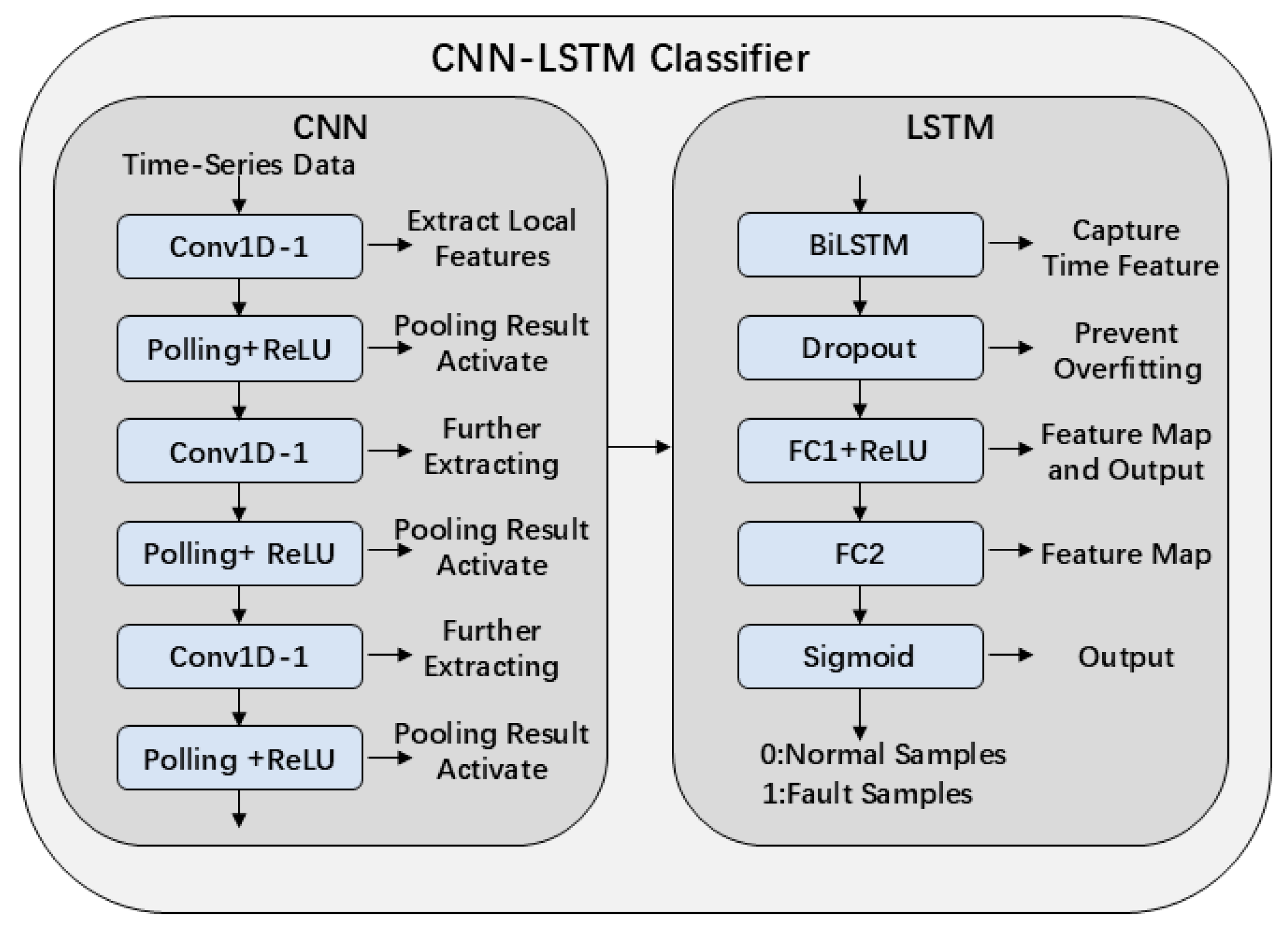
To effectively classify the augmented power battery operation data, this study constructs a deep learning model that combines a Convolutional Neural Network (CNN) with a Long Short-Term Memory (LSTM) network. This hybrid model leverages the ability of CNN to extract local features and the LSTM strength in modeling temporal dependencies, enabling fault detection within multivariate battery charging time-series data. The overall architecture of the model is illustrated in Figure 7.

The input format of this module is consistent with that used in the GAN model, namely, a multivariate time series with shape [256, 8]. Each sample contains 256 time steps and eight feature channels, corresponding to the following: voltage, current, State of Charge (SOC), maximum/minimum cell voltage, maximum/minimum cell temperature, and timestamp. The model outputs a probability value within the range [0, 1], indicating the likelihood that the sample represents a faulty charging process.

The model architecture consists of two main components: a CNN-based feature extraction module and a BiLSTM-based temporal modeling module.

In the CNN module, three sets of 1D convolutional layers (Conv1D) followed by max pooling operations are applied to progressively extract local temporal features from the input sequence. Each convolutional layer uses a kernel size of 3 and padding of 1 to capture local variations at different time scales—effectively detecting short-term patterns such as sudden voltage drops, SOC fluctuations, or abrupt temperature rises. Each convolutional layer is followed by a ReLU activation function to introduce non-linearity, and a max pooling operation to reduce the temporal dimension, thereby improving feature compactness and robustness.

In the LSTM module, the three-dimensional feature tensor output by the convolutional layers is reshaped to match the input requirements of the LSTM network and then passed into a bidirectional LSTM (BiLSTM) layer. This structure captures both forward and backward temporal dependencies, enabling the model to learn sequential patterns such as SOC progression, voltage oscillations, and other evolving trends during the charging process. The final hidden states from both directions of the BiLSTM are concatenated to form a global temporal feature representation.

The resulting temporal feature vector is fed into a two-layer fully connected network. The first layer applies non-linear compression and incorporates dropout regularization to reduce the risk of overfitting. The final layer uses a Sigmoid activation function to output a scalar probability indicating whether the current sample is classified as a fault. The specific network layer details and parameter settings for each layer of module are shown in

Table 3. CNN-LSTM classification network architecture and settings.

Module	Content	Parameter Setting	Output Size (B = Batch Size)
CNN	Input (Time-series data) Permute Conv1D-1	in channels = 8 out channels = 32 kernel size = 3 padding = 1	(B, 256, 8) (B, 8, 256) (B, 32, 256)
	MaxPool1D	kernel_size = 2	(B, 32, 128)
	Conv1D-2	in channels = 32 out channels = 64 kernel size = 3 padding = 1	(B, 64, 128)
	MaxPool1D	kernel_size = 2	(B, 64, 64)
	Conv1D-3	in channels = 64 out channels = 128 kernel size = 3 padding = 1	(B, 128, 64)
	MaxPool1D	kernel_size = 2	(B, 128, 32)
LSTM	Permute BiLSTM	input size = 128 hidden size = 64	(B, 32, 128) (B, 32, 128) (B, 128)
	Dropout	p = 0.5	(B, 128)
	FC-1 + ReLU	input size = 128 output size = 64	(B, 128) (B, 64)
	FC-2	input size = 64 output size = 1	(B, 64)
	Sigmoid	output size = 1	(B, 1)

.

The model is trained on the balanced dataset augmented by the GAN, with input samples in the form of time series with shape (256, 8), and outputs representing the probability of each sample being either faulty or normal. The binary cross-entropy (BCE) loss function—consistent with that used in the GAN module—is employed for optimization. BCE loss is widely recognized as the standard loss for binary classification tasks, as it measures the divergence between the predicted probability distribution and the true labels, and provides well-behaved gradients that facilitate stable and efficient model training [28]. The Adam optimizer is selected, with an initial learning rate of 0.001, and the batch size is set to 64.

In the subsequent experimental section, this model will be compared with other classification approaches to evaluate its performance in the task of power battery fault detection.

5. Experiments and Results

5.1. Experimental Setup and Evaluation Metrics

To validate the effectiveness of the proposed GAN-based data augmentation method and the CNN-LSTM classification model in power battery fault detection, a series of experiments were conducted using a real-world dataset collected from new energy vehicles. All experiments follow a standard train/validation/test split strategy to ensure stable training and comprehensive evaluation of model performance.

All experiments were implemented using the PyTorch 2.4.1 framework and conducted on a workstation equipped with an NVIDIA GPU.

Prior to training, the original dataset was divided into three subsets: train set, validation set, test set. The test set remained untouched during both training and data augmentation, preserving the original data distribution for fair and objective performance evaluation. From the training set, all normal samples and labeled fault samples were extracted separately. The fault samples were used as real anomaly data to train the GAN model, enabling it to learn the latent distribution of abnormal sequences. Subsequently, the trained generator was used to produce synthetic fault samples, increasing the number of fault instances to approximately match the number of normal samples, thereby achieving class balance.

Finally, the synthetic fault samples, real fault samples, and normal samples were combined to form a balanced training set, which was used to train the CNN-LSTM classification model. During training, the loss value and accuracy metrics were monitored in real-time on the validation set to guide decisions on the number of training epochs and optimization strategy, helping to prevent overfitting. After training, the model was evaluated on the test set to assess its final performance.

To comprehensively evaluate the classification performance of the model, four commonly used binary classification metrics are adopted: Accuracy, Precision, Recall, and F1-Score. Accuracy measures the proportion of correctly predicted samples among all samples. Precision evaluates the proportion of correctly identified fault samples among all samples predicted as faulty. Recall assesses the proportion of actual fault samples that are successfully detected by the model. F1-Score is the harmonic mean of precision and recall, serving as an important metric for balanced performance evaluation.

The mathematical definitions of these metrics are as follows Equations (5)–(8):

$$Accurany={\displaystyle \frac{TP+TN}{TP+TN+FP+FN}}$$

(5)

$$Precision={\displaystyle \frac{TP}{TP+FP}}$$

(6)

$$Recall={\displaystyle \frac{TP}{TP+FN}}$$

(7)

$$F1=2\times {\displaystyle \frac{Precision\times Recall}{Precision+Recal}}$$

(8)

where:

• $TP$ (True Positive): the number of fault samples correctly predicted as faulty.
• $TN$ (True Negative) the number of normal samples correctly predicted as normal.
• $FP$ (False Positive): the number of normal samples incorrectly predicted as faulty.
• $FN$ (False Negative): the number of fault samples incorrectly predicted as normal.

In imbalanced classification tasks, models tend to learn the characteristics of the majority class (i.e., normal samples) more easily, often leading to high accuracy for normal samples but poor detection of fault samples. Given that this study focuses on identifying abnormal battery behavior, the Precision, Recall, and F1-Score of the positive class (fault samples) are considered the core evaluation metrics, reflecting the model’s practical effectiveness in fault detection.

5.2. Fault Detection Experiments Based on the Generative Adversarial Network with a Convolutional Long Short-Term Memory (GAN-CNN-LSTM)

To evaluate the effectiveness of the proposed GAN-CNN-LSTM-based method for power battery fault detection, we first divided the full dataset into training, validation, and test sets in a 6:2:2 ratio. The test set remained fixed throughout the experiments and was not subjected to any data augmentation. After splitting, the training set contained 17,033 samples, and the validation set contained 5678 samples. Within the training set, 14,241 were normal samples and 2792 were fault samples. The test set also contained 5678 samples.

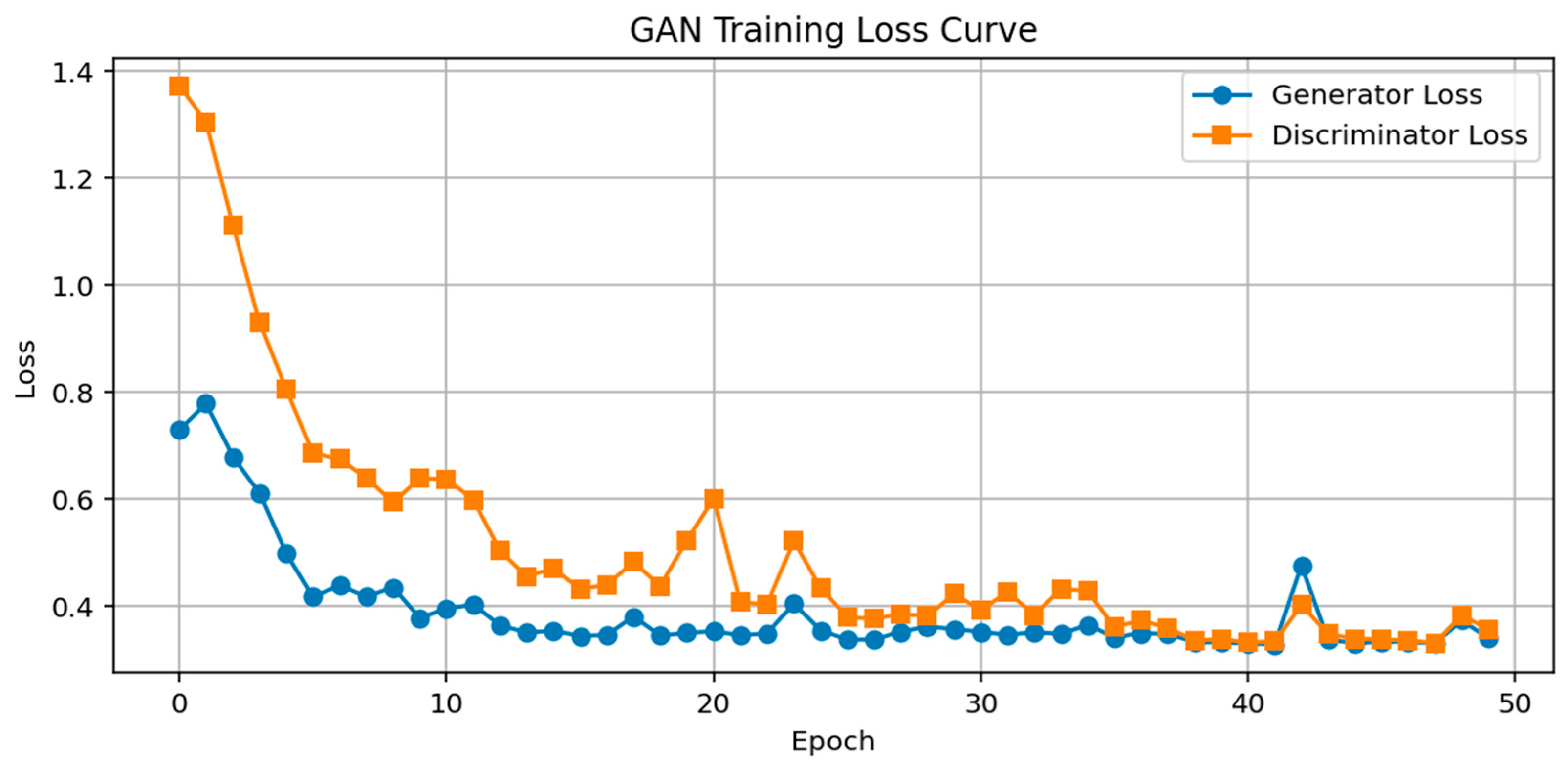
The proportion of fault samples is relatively low, resulting in significant class imbalance in the training data. To address this issue, we constructed a GAN model as detailed in Figure 6 and trained it using all fault samples extracted from the training set. As shown in Figure 8, after 25 training epochs, the loss curves of both the generator and discriminator stabilized with mild oscillations, indicating that the adversarial training reached a balanced state. At this point, the generator was able to produce synthetic data resembling real fault samples, while the discriminator found it increasingly difficult to distinguish between real and fake data.

To balance the training set, we calculated the shortfall in fault samples relative to normal samples (11,449 samples) and determined the number of synthetic samples needed. By feeding random noise into the trained generator, we generated 11,449 synthetic fault samples, which were then combined with the real fault samples and the normal samples to construct a balanced training set of 28,482 samples for subsequent model training and evaluation.

In our experiments, the GAN model was trained for 50 epochs. This number was determined based on preliminary trials, where both the training and validation loss curves were observed to stabilize within about 50 epochs, and the quality of the generated samples became comparable to the real samples. Further increasing the number of epochs resulted in negligible improvements but increased computational costs.

To intuitively demonstrate the effectiveness of the trained GAN in generating realistic fault samples, we visualized the distributions of real and synthetic samples using both t-SNE and PCA (see Figure 5). t-SNE and PCA provide non-linear and linear dimensionality reduction, respectively, allowing for the visualization of high-dimensional data in two-dimensional space. As shown in Figure 9, the distributions of the fake samples (yellow) and the real samples (blue) largely overlap, indicating that the generator successfully captures the key characteristics of the real fault data and is able to produce high-quality synthetic samples. This also suggests that our GAN does not suffer from severe mode collapse during training.

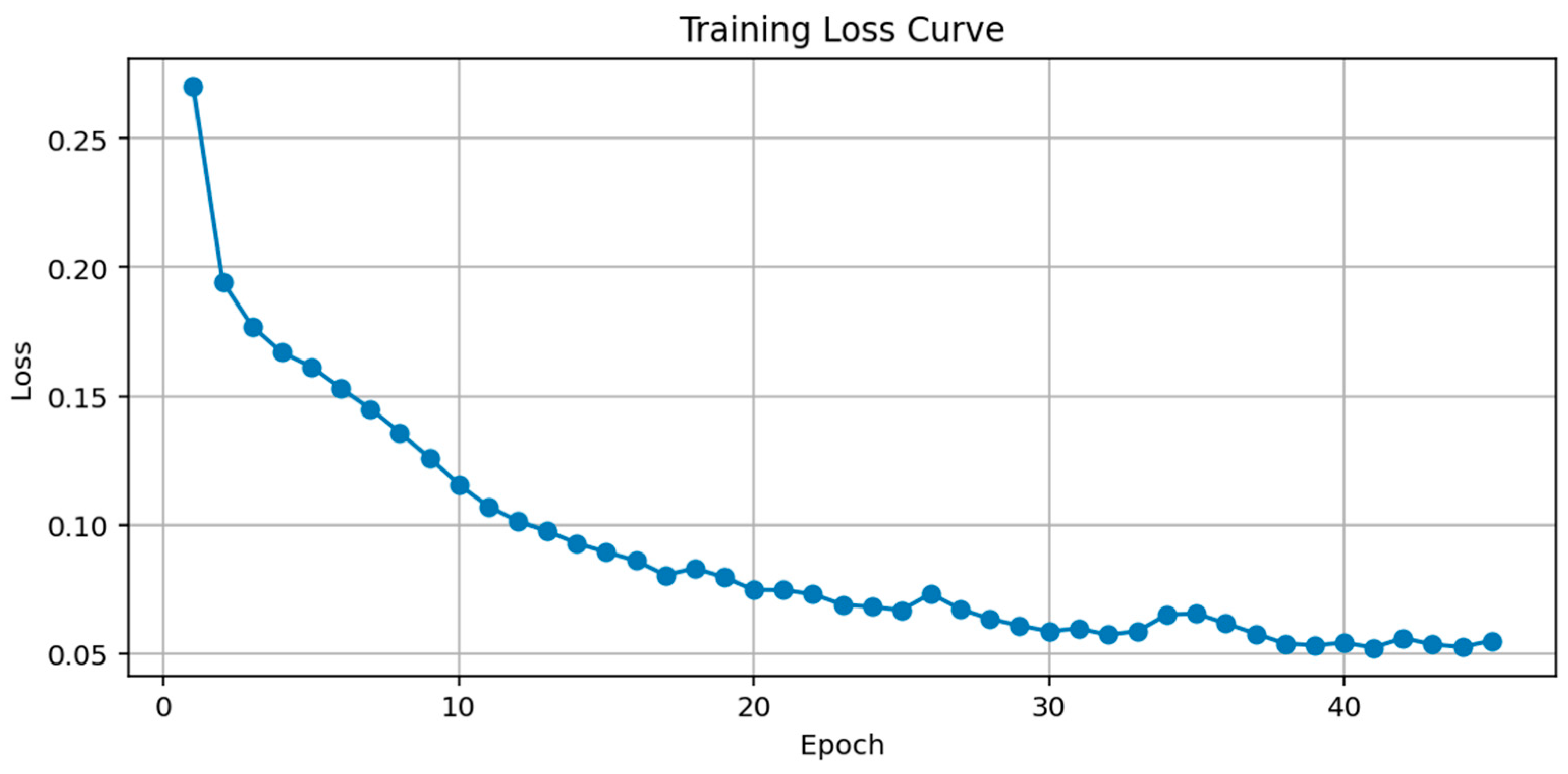
To verify the effectiveness of the CNN-LSTM classification module within the GAN-CNN-LSTM framework, we trained the classifier using the balanced dataset constructed above. As shown in Figure 10, after approximately 30 training epochs, the model’s loss values stabilized with slight fluctuations, indicating convergence and a stable training process.

Next, we fed the fixed test set into the trained classifier to evaluate its fault detection capability. The test results are summarized in

Table 4. Classification results of the GAN-CNN-LSTM model on the test set.

Label	Precision	Recall	F1-Score	Accuracy
0	97.56%	99.18%	98.36%	97.23%
1	95.38%	87.23%	91.12%

, reflecting the model’s classification performance across different sample types.

We separately recorded the model’s classification metrics on both normal samples and fault samples (i.e., positive class). For normal samples, the Precision, Recall, and F1-Score all exceeded 97%, and the overall test Accuracy reached 97.23%. More importantly, for the fault detection task, which is the primary focus of this study, the model achieved a Precision of 95.23%, Recall of 87.23%, and a comprehensive F1-Score of 91.12% on the positive class—demonstrating strong performance in identifying fault samples.

To further validate the classification performance of the proposed model, we plotted the PR (Precision-Recall) curve and ROC (Receiver Operating Characteristic) curve of the GAN-CNN-LSTM model, as shown in Figure 11. The trends of these curves indicate that the proposed model demonstrates excellent classification performance in the fault detection task.

Furthermore, to assess the stability and reliability of the proposed GAN-CNN-LSTM model, a bootstrap analysis (n = 1000) was conducted to estimate the confidence interval for the AUC metric. The results show that the average AUC of GAN-CNN-LSTM is 0.9927, with a 95% confidence interval of [0.9909, 0.9942], indicating highly robust and consistent fault detection performance on the test set.

To assess the deployment feasibility of the proposed model, we measured the inference time and model size on a workstation equipped with an NVIDIA RTX 4090 GPU and an Intel i9-14900K CPU (single-threaded, batch size = 1, sequence length = 256, feature dimension = 8). The average inference time per sample is approximately 0.44 milliseconds on the CPU, and the total number of model parameters is 81,889. Given that typical BMS systems have data acquisition intervals of several seconds, our model’s latency is orders of magnitude faster than real-time requirements, making it well-suited for integration into embedded or edge computing environments in battery management systems.

In summary, the proposed GAN-CNN-LSTM model exhibits outstanding overall classification accuracy and, more critically, shows high robustness and practical utility in detecting battery faults. These results validate the model’s effectiveness in the power battery fault detection task.

5.3. Comparative Experiments with Deep Learning Models

To further validate the advantages of the proposed model, we designed three groups of comparative experiments to assess the fault detection performance of different deep learning architectures without data augmentation. The three configurations tested are as follows:

• A CNN-LSTM classifier trained without GAN-based data augmentation;
• A classifier using only CNN;
• A classifier using only LSTM.

All models were trained on the original (imbalanced) training set, while the test set remained fixed, consistent with the previous GAN-CNN-LSTM experiment. The network structures of each model were kept consistent with their respective components in the GAN-CNN-LSTM model, with only minor adjustments to input dimensions to satisfy CNN or LSTM input requirements. The final results are summarized in

Table 5. Comparative classification results of deep learning models.

Model	Label	Precision	Recall	F1-Score	Accuracy
CNN-LSTM	0	97.08%	95.01%	96.03%	93.43%
	1	76.88%	85.28%	80.86%
CNN	0	94.70%	98.57%	96.60%	94.19%
	1	90.68%	71.65%	80.05%
LSTM	0	94.65%	97.08%	95.85%	92.96%
	1	82.67%	71.75%	76.83%

.

Experimental results show that all three models achieved strong performance on the negative class (normal samples), with overall Accuracy around 95%. However, their performance on the positive class (fault samples) varied significantly, making this the primary focus of our analysis.

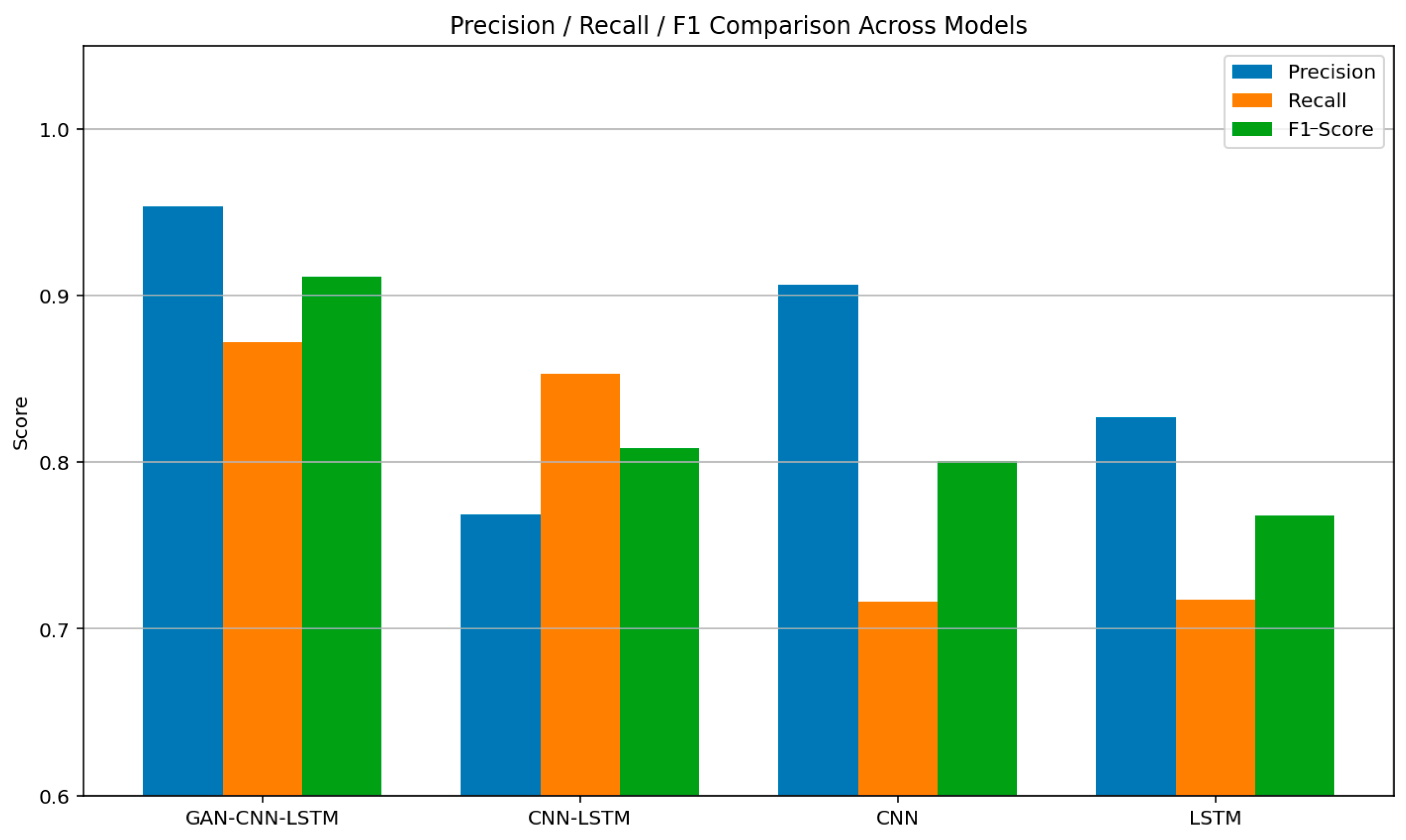
As illustrated in Figure 12, we compared the GAN-augmented CNN-LSTM model with the above three models. After data augmentation, the classification metrics on fault samples significantly improved. Notably, Precision increased from 76.88% to 95.38%, indicating a substantial improvement in the model’s ability to accurately identify fault samples. Recall improved by approximately 2%, and the F1-Score increased by about 11%, confirming that data augmentation greatly enhanced the model’s detection capability for the positive class. This experiment strongly supports the effectiveness of using GAN-based sample generation to address the class imbalance problem.

Additionally, a comparison among the three deep learning architectures shows that the CNN-LSTM model outperformed both CNN and LSTM when detecting fault samples, achieving an F1-Score of 80.86%, compared to 80.05% for CNN and 76.83% for LSTM. Although the CNN-only model performed similarly in terms of F1-Score, its Recall was approximately 14% lower than that of the CNN-LSTM model, indicating limited sensitivity to fault samples. The LSTM model exhibited a similar limitation.

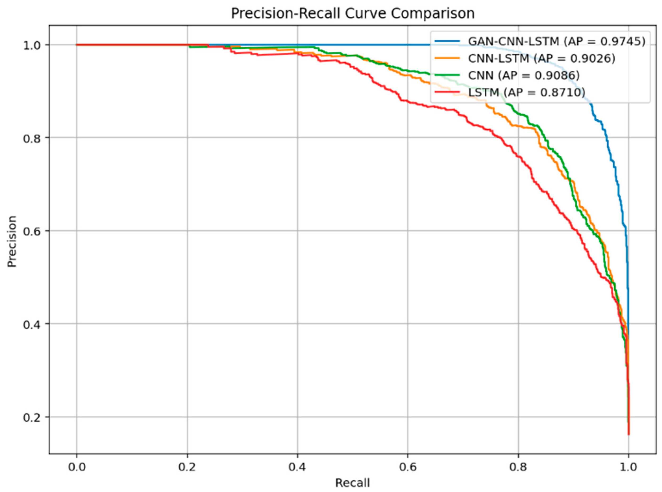
To further evaluate the models’ performance across different classification thresholds, we plotted the Precision-Recall (PR) curves and calculated the Average Precision (AP) for each model. As shown in Figure 13, the PR curve of the GAN-CNN-LSTM model encloses the largest area, with an AP of 0.9745, significantly higher than the other three models. The CNN-LSTM, CNN, and LSTM models achieved AP values of 0.9026, 0.9086, and 0.8710, respectively, with the LSTM model performing the worst.

These results further demonstrate the effectiveness of data augmentation in improving model stability and generalization capability. In particular, when dealing with imbalanced fault detection tasks, the GAN-CNN-LSTM model not only achieves superior F1-Score, Precision, and Recall at a fixed threshold, but also shows a clear advantage in overall classification ability as reflected by the PR curve.

In conclusion, the deep learning model comparison experiments clearly demonstrate the significant benefit of GAN-based data augmentation in enhancing the model’s ability to detect fault samples. Moreover, the CNN-LSTM architecture proves more effective than standalone CNN or LSTM models in capturing both temporal and spatial features of battery operation data.

5.4. Comparative Experiments with Machine Learning Models

As power battery operational data are inherently structured multivariate time-series data, traditional machine learning methods still possess a certain degree of modeling capability for such data. To further evaluate the advantages of the proposed approach, we conducted comparative experiments using five classical machine learning models: K-Nearest Neighbors (KNNs), Random Forest (RF), Naive Bayes (NB), Logistic Regression (LR), and Support Vector Machine (SVM).

Since traditional machine learning algorithms cannot directly process two-dimensional time-series inputs, we adopted a flattening approach to convert the data format. Specifically, each original sample with shape (256, 8) was flattened into a (1, 2048) vector. This transformation preserves as much temporal feature information as possible while satisfying the requirement of fixed-size inputs for machine learning models. Compared to statistical feature engineering, this method retains the structure of the original sequence without introducing significant manual bias.

The flattened training and test datasets were then used to train and evaluate the five machine learning models mentioned above. The same evaluation metrics—Precision, Recall, and F1-Score—used in the deep learning experiments were applied here for consistent comparison. The results are summarized in

Table 6. Comparative classification results of machine learning models.

Model	Label	Precision	Recall	F1-Score	Accuracy
Random Forest	0	93.99%	97.62%	95.77%	92.78%
	1	84.73%	67.86%	75.36%
Logistic Regression	0	90.26%	94.76%	92.46%	87.06%
	1	63.76%	47.40%	54.38%
Naive Bayes	0	90.21%	59.51%	71.71%	60.69%
	1	24.27%	66.77%	35.60%
KNN	0	95.73%	95.69%	95.71%	92.81%
	1	77.86%	98.03%	77.95%
SVM	0	94.26%	92.85%	93.36%	89.46%
	1	81.26%	51.75%	63.05%

.

Experimental results show that KNN and Random Forest performed relatively well in detecting fault samples, achieving F1-Scores of 77.95% and 75.36%, respectively, indicating a moderate capability for fault identification. In contrast, Naive Bayes yielded the worst performance, with an F1-Score of only 35.60%, indicating its inability to detect faults effectively.

Logistic Regression and SVM showed high classification performance on the negative class (normal samples), with Precision and Recall both exceeding 90%. However, their Recall scores on the positive class (fault samples) were only around 50%, suggesting that they struggle with fault detection—a critical task in this domain—and thus may fall short of practical application requirements.

In summary, although some traditional machine learning methods (such as KNN and Random Forest) achieved modest performance on structured fault data, their overall classification capabilities remain significantly inferior to deep learning models like GAN-CNN-LSTM, particularly in terms of detecting fault samples. These results further confirm the advantage of deep learning models in capturing complex temporal and spatial patterns in power battery operational data.

5.5. Overall Performance Comparison of Models

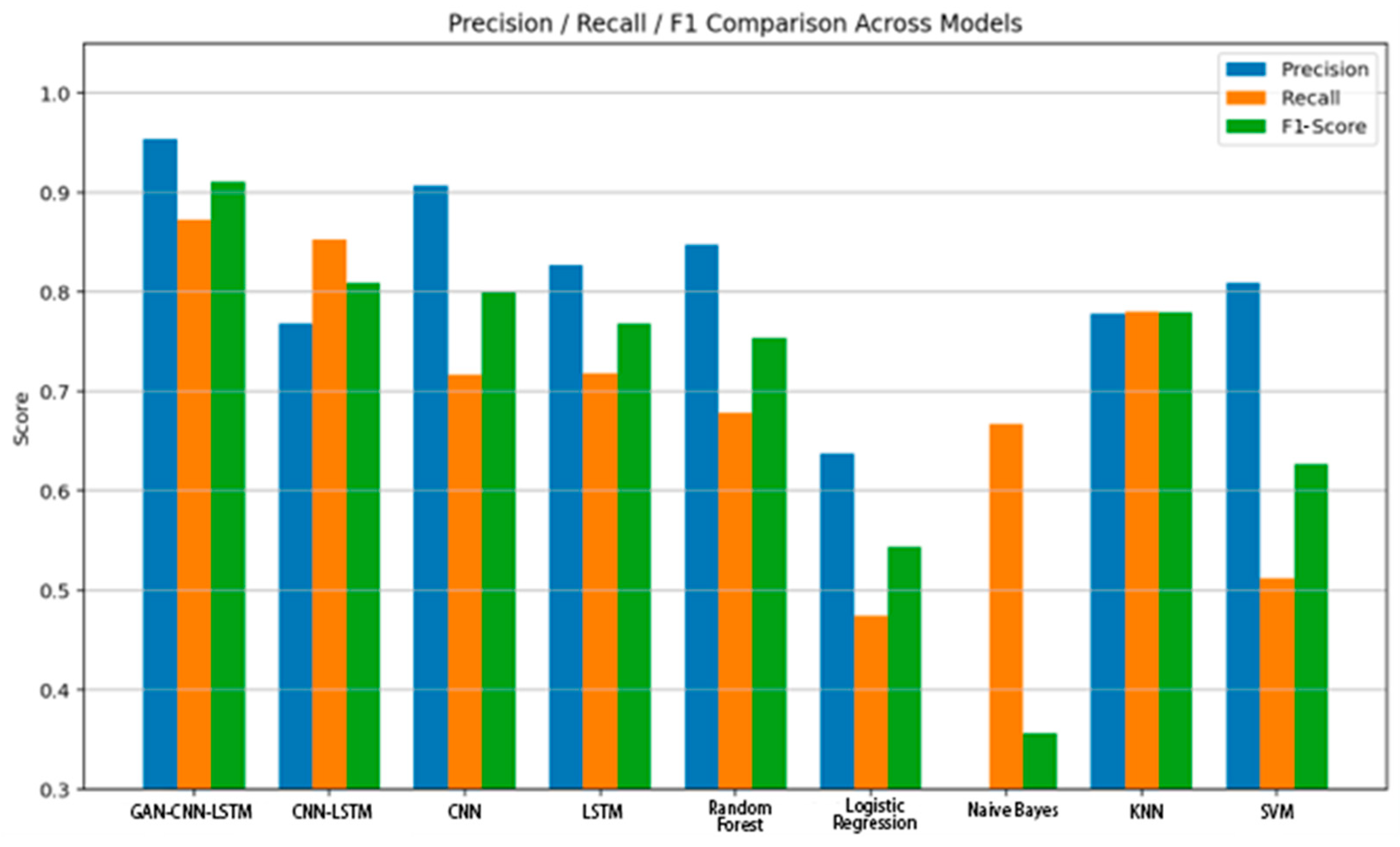
To more intuitively demonstrate the performance advantages of the proposed GAN-CNN-LSTM model in the task of power battery fault detection, we present a consolidated summary of the key experimental results. As shown in Figure 14, the GAN-CNN-LSTM model achieved the highest scores across all three key metrics—Precision, Recall, and F1-Score—significantly outperforming both the other deep learning models and traditional machine learning models.

A comparison between deep learning and traditional machine learning models reveals that, although certain machine learning methods (e.g., Random Forest and KNN) show some classification capability for structured battery operation data, their overall detection performance remains noticeably lower than that of deep learning models capable of directly modeling time-series features.

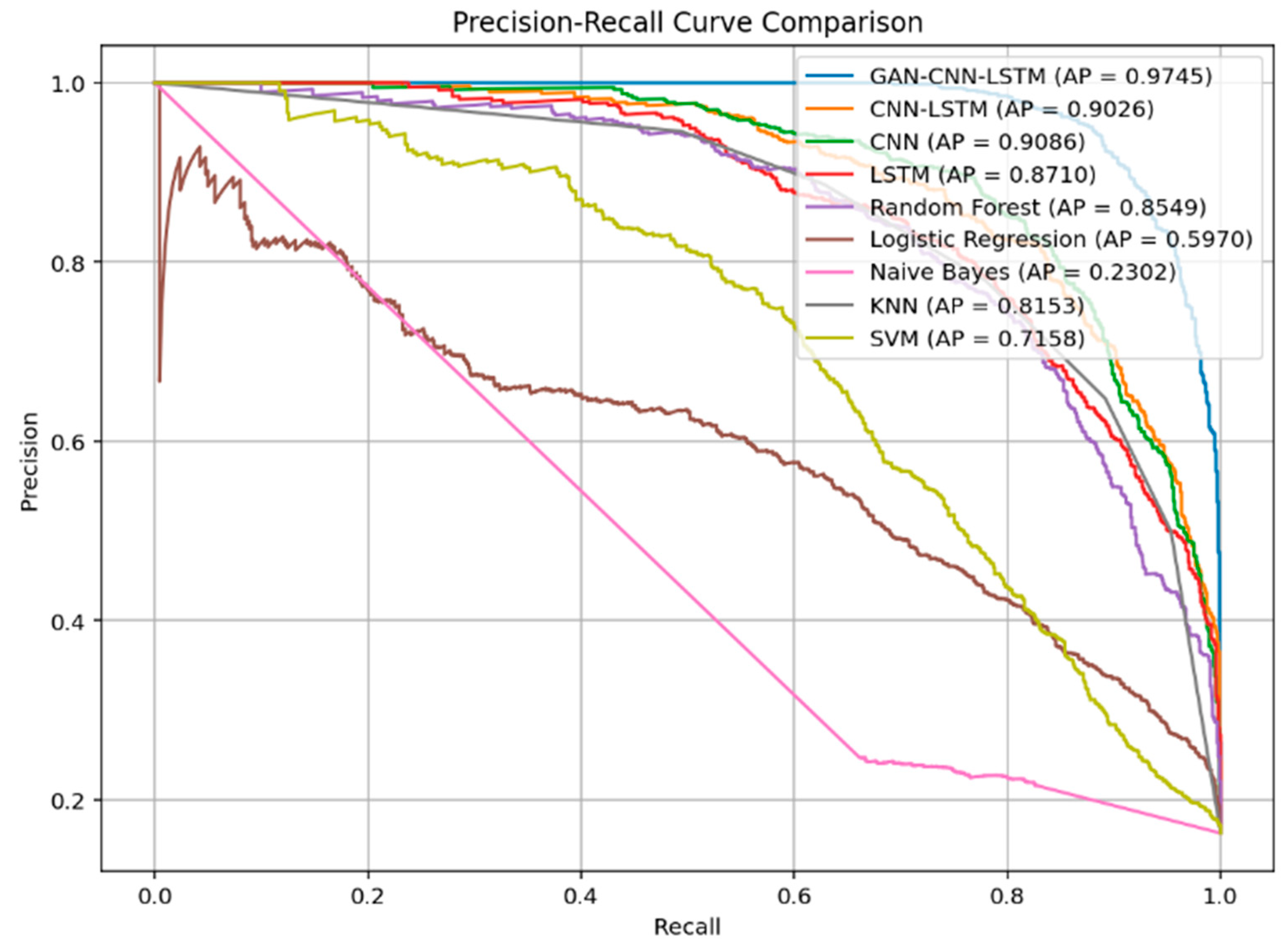
Furthermore, we plotted the Precision-Recall (PR) curves and Receiver Operating Characteristic (ROC) curves for all models, as shown in Figure 15 and Figure 16, respectively. Among the machine learning models, Random Forest achieved the highest Average Precision (AP) at 85.49%, while Naive Bayes performed the worst with an AP of only 0.23. In contrast, even the lowest-performing deep learning model (LSTM) achieved an AP of 87.10%, which still exceeded the performance of all traditional methods.

The results of the ROC curves further support this trend. All deep learning models achieved higher Area Under the Curve (AUC) values than their machine learning counterparts. Notably, the GAN-CNN-LSTM model reached an AUC of 0.99, the highest among all models tested, demonstrating its outstanding discrimination capability in the fault detection task.

To quantitatively evaluate whether the proposed GAN-CNN-LSTM model significantly outperforms baseline methods, we performed statistical significance testing on the Area Under the ROC Curve (AUC) using the bootstrap resampling method (n = 1000). As shown in

Table 7. Bootstrap test results.

Model	Mean_Diff	CI_Lower	CI_Upper
CNN-LSTM	0.018	0.015	0.022
CNN	0.019	0.015	0.023
LSTM	0.027	0.023	0.031
Random Forest	0.034	0.029	0.039
Logistic Regression	0.116	0.105	0.127
Naive Bayes	0.338	0.323	0.355
KNN	0.043	0.037	0.052
SVM	0.116	0.103	0.130

, for each comparison between GAN-CNN-LSTM and the baseline models—including CNN-LSTM, CNN, LSTM, Random Forest, Logistic Regression, Naive Bayes, KNN, and SVM—the mean difference in AUC, along with its 95% confidence interval, was calculated.

For all comparisons, the mean AUC difference was positive, and the 95% confidence intervals did not include zero. For example, the AUC of GAN-CNN-LSTM exceeds that of CNN-LSTM by an average of 0.018 (95% CI: 0.015–0.022), and exceeds Random Forest by 0.034 (95% CI: 0.029–0.039). The improvement over Naive Bayes is even larger, with a mean difference of 0.338 (95% CI: 0.323–0.355). These results demonstrate that the proposed model achieves robust and significant gains in fault detection performance compared with both deep learning and classical machine learning baselines.

In summary, the proposed GAN-CNN-LSTM model, enhanced through GAN-based data augmentation, exhibits clear advantages in handling structured time-series data. By effectively mitigating the class imbalance problem through fault sample generation, the model significantly outperforms unaugmented CNN, LSTM, and CNN-LSTM combinations, as well as traditional machine learning methods, in terms of both classification performance and robustness for power battery fault detection.

6. Conclusions and Future Work

With the rapid adoption of new energy vehicles, power battery safety has become an increasingly important research focus. Among related technologies, fault detection plays a critical role in ensuring the stable operation of battery systems and is gaining attention as a prominent topic in the academic community. In recent years, data-driven deep learning methods have shown great potential in battery fault detection. However, two major challenges remain in practical applications:

(1)

the strong temporal dependencies inherent in battery data;

(2)

the extreme scarcity of fault samples, leading to severe class imbalance.

To address these challenges, this paper proposes a GAN-CNN-LSTM-based deep learning fault detection model. The model takes real-world charging process data from electric vehicles as input and automatically learns both spatial and temporal features to determine whether a battery fault has occurred. The GAN module generates high-quality synthetic fault samples by learning the distribution of a small number of real fault cases, thereby balancing the dataset. The CNN-LSTM module directly models the multivariate time-series input—without the need for feature extraction or flattening—preserving the original structure and enabling efficient classification.

Experiments were conducted on a real-world dataset collected from battery operations. Results demonstrate that the proposed model achieved excellent fault detection performance. For fault samples (positive class)—the core target—the model achieved a Precision of 95.23%, Recall of 87.23%, and F1-Score of 91.12%, all significantly outperforming baseline models. For normal samples, all three metrics exceeded 97%. In addition, the model achieved outstanding results under PR and ROC curve evaluations, with an Average Precision (AP) of 97.45% and Area Under the Curve (AUC) of 99.00%, further validating its strong detection capability and overall classification performance.

Despite these promising results, this study still has certain limitations. First, the proposed model has not yet been deployed and validated in real vehicle environments. In future work, we plan to integrate the model into actual Battery Management Systems (BMSs) and evaluate its stability under dynamic operational conditions.

Second, the dataset used in this study is derived from a single manufacturer and vehicle type. This may limit the generalizability of the model to other vehicles or usage scenarios. Therefore, we aim to expand our dataset to include data from multiple manufacturers, vehicle types, and driving conditions, in order to systematically evaluate and enhance the robustness and transferability of the proposed method.

Additionally, combining mechanism-based diagnostic methods with data-driven models could help establish a multi-modal, hierarchical fault detection framework, further improving the model’s generalizability and practical utility in complex real-world scenarios.