Article

Supersonic Pulse-Jet System for Filter Regeneration: Molecular Tagging Velocimetry Study and Computational Fluid Dynamics Validation

1
Dominion Engineering, 12100 Sunrise Valley Dr., Suite 220, Reston, VA 20191, USA
2
Department of Mechanical and Aerospace Engineering, The George Washington University, 800 22nd Street NW, Washington, DC 20052, USA
3
Department of Nuclear Engineering and Radiological Sciences, University of Michigan, 2355 Bonisteel Blvd., Ann Arbor, MI 48109, USA
*
Author to whom correspondence should be addressed.
Current address: Metroscope Inc., 201 N Union St Suite 110, Alexandria, VA 22314, USA.
Current address: MPR Associates, 320 King St, Alexandria, VA 22314, USA.
Appl. Sci. 2025, 15(10), 5764; https://doi.org/10.3390/app15105764
Submission received: 10 April 2025 / Revised: 7 May 2025 / Accepted: 16 May 2025 / Published: 21 May 2025
(This article belongs to the Section Fluid Science and Technology)

Abstract

:

Featured Application

The validated CFD model and accompanying experimental insights presented in this study are directly applicable to the design and optimization of pulse-jet cleaning systems used in industrial gas filtration. By providing high-resolution velocity and shock structure data, this work supports improved modeling accuracy, which can lead to enhanced cleaning efficiency, reduced energy consumption, and extended filter life in industrial applications.

Abstract

This paper provides shadowgraphy and molecular tagging velocimetry (MTV) acquisition results and validates a computational fluid dynamics (CFDs) simulation for an underexpanded supersonic gas jet in a plenum pointed toward a wall with an aligned converging pipe outlet. Flow configurations of this type are encountered in pulse-jet systems for online industrial gas filter regeneration. Although previous CFD validation efforts for pulse-jet systems have relied on static pressure measurements, this work expands the validation data using high-resolution flow visualization and velocimetry techniques. Simulations were performed with an axisymmetric two-dimensional Reynolds-averaged Navier-Stokes model and are in close agreement with the shadowgraphy and MTV data, including the description of Mach disks, barrel shocks, and reflected shocks in the underexpanded jet. The CFD model was finally applied to study the role of the converging tube downstream of the jet.

1. Introduction

This work studies the flow configuration of a supersonic gas jet in a plenum pointed toward a wall with a converging outlet pipe opening aligned with the jet. This configuration is industrially relevant for pulse-gas filter regeneration systems that perform periodic backwash pulses to remove solid cake from the filtering media.
In these systems, gas pulses lasting less than a second (50 to 1000 ms) are directed toward the filtering media in the reverse direction compared to the filtration process to enable backwash of the media. This regeneration [1] is performed without interrupting the main process flow, cleaning a subset of the total filtering media each time. Such an online regeneration capability allows the avoidance of periodic shutdowns and manual disassembly to clean the filters. The capability of regenerating the filters during operation is especially desirable in systems processing hazardous materials or in systems with a high loading rate of solid particulates in the gas.
The optimization of pulse-jet system designs often relies on prototyping and testing. However, the adoption of computational fluid dynamics (CFDs) reduces the cost of individual steps in parametric exploration, thus allowing enhanced optimization at a reduced cost.
The suitability of CFD for pulse-jet applications has been supported by numerous validation studies. The studies often tested two-dimensional or three-dimensional Reynolds-averaged Navier–Stokes (RANS) models against pressure measurements collected in pulse-jet system experiments [2,3,4]. The present work extends CFD validation to flow visualization and velocity measurements acquired inside the supersonic jet through a combination of shadowgraphy and velocimetry. To the best knowledge of the authors, this paper presents the first application of high-resolution measurements for a filter pulse-jet configuration.
Flow velocity is measured with molecular tagging velocimetry (MTV). MTV is an optical time-of-flight technique that transforms fluid molecules into temporary tracers through resonance excitation by photons (of a set wavelength). While particle image velocimetry (PIV) requires the injection of solid particles acting as tracers, in MTV, the gas molecules themselves are converted into tracers; thus, the inertial effects on tracers are minimal, and shock waves are captured faithfully.
MTV techniques (under different names) have been widely used to measure supersonic gas jets [5,6,7]; see Pitz and Danehy [8] for a recent detailed review. Similarly, CFD methods have been widely compared with high-resolution data in supersonic jets [9].
Prior CFD validations for pulse-jet configurations have focused mainly on systems with fabric filters, displaying challenges in accurately predicting pressure in the ramp-down period as the filter deforms [3]. This work focuses on solid-mesh filters. Fabric filters can be backwashed more easily than solid-mesh filters because pulse jets cause the fabric to inflate and reach its elastic limit, resulting in rapid deceleration and release of accumulated cake. However, fabric filters are not suitable for high-temperature (hot gas) filtration, for which rigid self-supporting media are necessary to ensure mechanical, chemical, and thermal stability [1]. Backwash of solid-mesh filters relies solely on the direct interaction between the fluid flow and the filter cake, which is established through design optimization.
The performance of backpulse in solid filters has been extensively evaluated in the literature based on theoretical and experimental evaluations [10] and the evaluation of effects on the filter cake [11].
A key component of the backpulse system, whose role has been debated, is the pipe connecting the filter outlet flange to the downstream plenum (defined considering the direction of normal filtration). This pipe is present in systems with both fabric and solid-mesh filters and industrially referred to as a “Venturi” due to the commonly encountered converging–diverging cross-section. However, the shape of the Venturi varies between systems: the device is sometimes a straight pipe. The goal of the Venturi is to maximize the effect of the pulse jet, allowing the jet and the entrained gas to enter the filter but not easily escape, and at the same time ensuring a low-pressure drop during normal operation [12]. Furthermore, in hot gas filters, the Venturi helps mix between cold pulse jet gas and hot fluid entrained to reduce the thermal stresses on the filter compared to direct exposure to cold gas [1]. Liu and Shen [13] and Liu and Shen [13] evaluated theoretically and experimentally the performance of different Venturi geometries in terms of pressure versus flow rate for fabric filters.
The system studied in this paper, hereby called “reference system”, is the process gas filter component of the Integrated Waste Treatment Unit (IWTU) in Idaho, United States. This facility treats a highly contaminated gaseous waste stream at a temperature over 550 °C and uses silicon carbide filtering media.

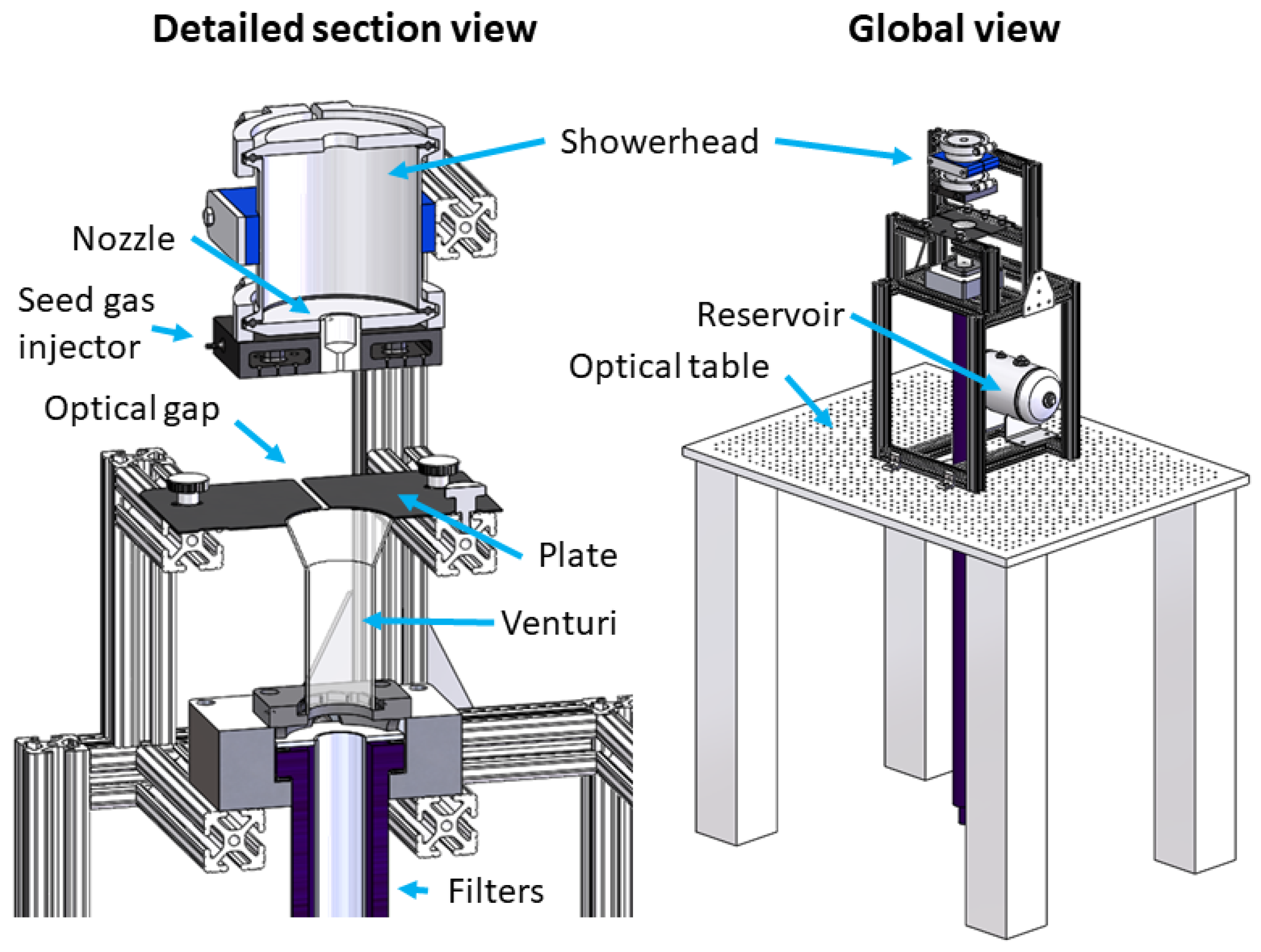
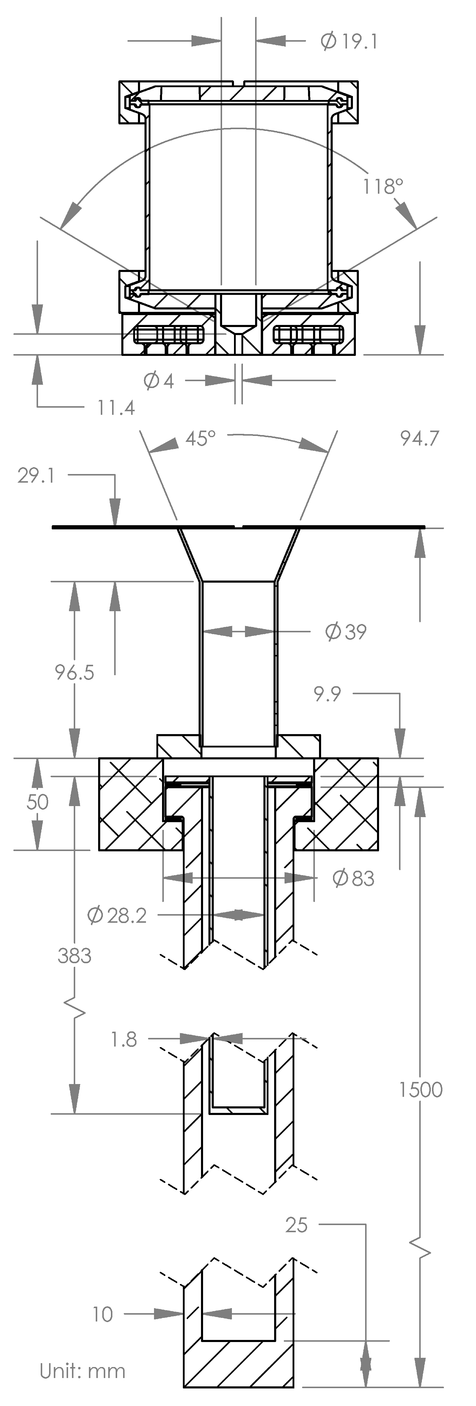
2. Experimental Setup

2.1. Test Rig

Experimental acquisitions were performed using a test rig that replicates at full scale the geometry of a single filter element in the reference industrial system. The rig operates at ambient temperature but at the same (ambient) pressure encountered in the reference system.
Figure 1 shows the experimental rig. The supersonic nozzle is mounted at the bottom of a plenum or “showerhead” and faces down toward the Venturi. The Venturi sits above the throat of the filter housing.
As shown in Figure 2, the nozzle throat has the geometry of a 4 mm diameter, 11.4 mm long tube. Upstream of that throat is a cone with a 118 angle opening. When a solenoidal valve is triggered, high-pressure gas from a 3.9-L reservoir is released into the showerhead, producing a supersonic jet past the nozzle. 12.7 mm (1/2 in) tubing (1 m long) connects the reservoir to the 0.85-L showerhead. The MTV seed gas, chosen as N 2 O , is mixed in low concentration with the compressed air in the reservoir when the reservoir is filled.
Below the showerhead, a plastic “seed gas injector” built through additive manufacturing injects N 2 O through small holes at very low flow rates. This injection ensures that the volume surrounding the jet is also seeded. This is necessary for MTV to resolve the flow entrained and mixed by the jet. This is particularly important for measurements in the far field of the nozzle, i.e., near the Venturi entrance.
The so-called Venturi is a conical converging channel followed by a straight segment; it is located 94.7 mm downstream of the nozzle exit. The conical angle is 45 . To enable probing the flow inside the Venturi, the latter was fabricated out of thin-wall UV-transparent fused quartz, which guarantees a 70% transmittance for MTV conducted there. A flat plate around the top of the Venturi seals the air path that would bypass the Venturi’s entrance. The plate contains a narrow gap needed as a path for lasers used in velocimetry acquisitions.
Downstream of the Venturi, two concentric filter candles are present: an inner stainless steel filter and an outer silicon carbide one. During normal filter operation, gas would flow radially from the outside to the inside and then axially to the downstream plenum, resulting in the accumulation of solid particulate on the outside surface. When regeneration is triggered, the pulse jet is directed axially to the internal cavity of the cylindrical filter from the downstream “clean side” plenum, causing reverse mass flux through the filter mesh and filter regeneration. The porous viscous resistance across each of the two filters is available from the manufacturers as indicated below. Respectively, for the inner and outer filter:
Δ p ρ ν u = 1.4 × 10 8 m 1 ,
Δ p u = 81,434 kg m 2 s 1 .
Both equations include pressure drop Δ p and velocity u, and the first one also includes density ρ and kinematic viscosity ν .

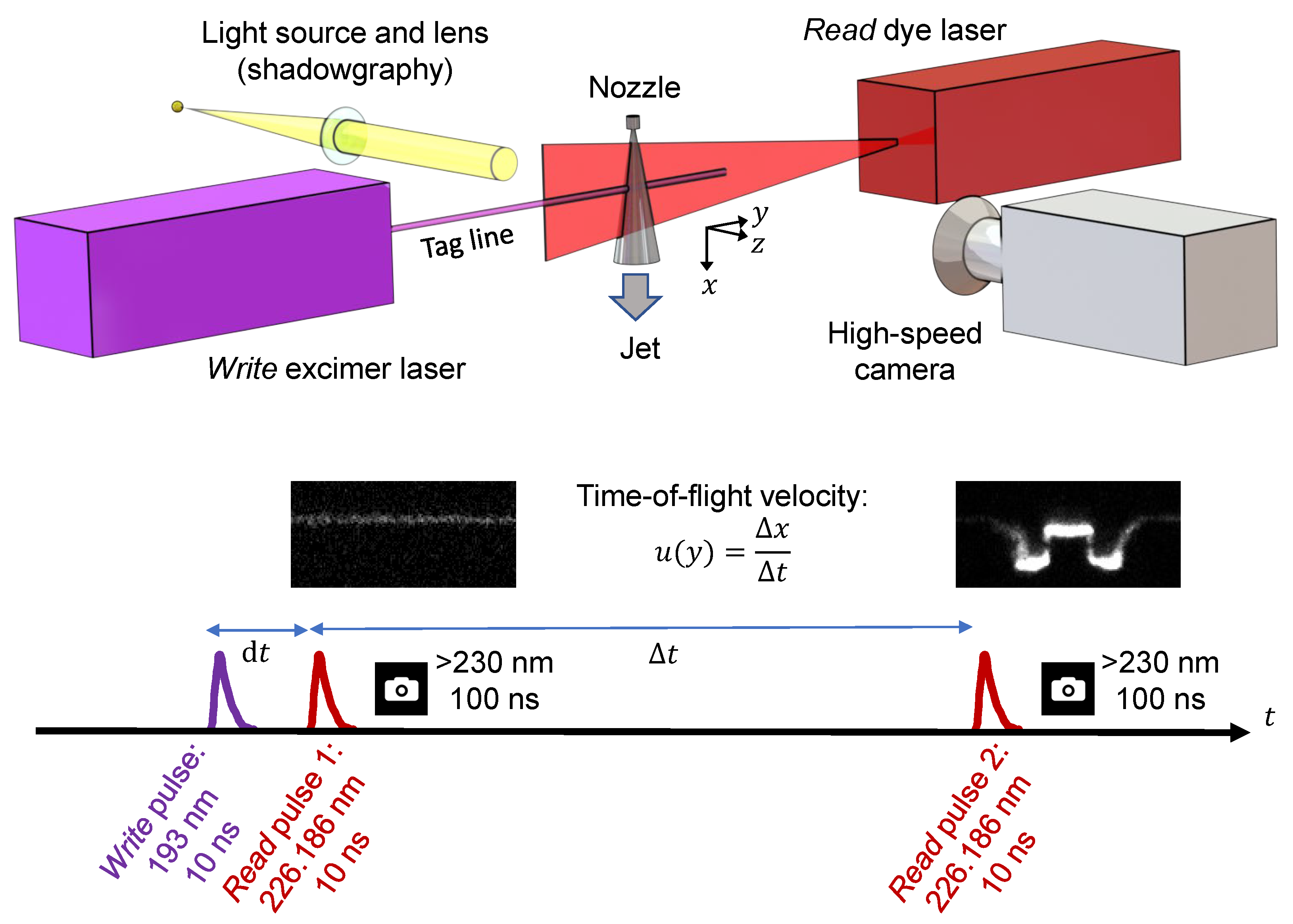
2.2. Shadowgraphy Configuration

Flow visualization inside the jet is performed using a shadowgraphy setup. A lens is used to direct light from an intense source through the supersonic jet normal to the direction of the flow and then into a high-speed camera (Phantom v710). The light source and camera are at a sufficiently long distance from the flow such that light can be considered collimated. This configuration is illustrated in the upper left portion of Figure 3. Nonuniformities in transparent air, such as shock waves, display large variations in refractive index; those regions appear dark (shadows) on a bright illuminated background. The camera acquires images at a rate of 9000 frames per second with a 512 × 384 pixel field of view (FOV) and a magnification of 0.11 mm/pixel. The images in Figure 4 are cropped to 6.8 × 20 mm 2 and averaged over 90 instantaneous frames (10 ms).

2.3. Molecular Tagging Velocimetry Configuration

The MTV configuration adopted for this work is illustrated in Figure 3 and briefly described here; more details are available in André et al. [14]. A nitrous oxide ( N 2 O ) seed gas is premixed with the pulse gas (compressed air) and dispersed around the jet region before the pulse. A write 10-ns 193-nm ArF excimer laser pulse decomposes molecules of N 2 O via photodissociation and creates NO tracers with a predetermined regular spatial pattern, such as a horizontal line across the jet. Then, a read tunable dye laser with a wavelength of 226.186 nm and a pulse duration of 10 ns is triggered within a short time interval d t from the write laser on a cross section of the flow to induce fluorescence of the NO tracer molecules formed through the write step. Both lasers operate at 10 Hz, and the beam energy at the jet location is 5 mJ/pulse and 0.5 mJ/pulse for the write and the read laser, respectively.
The location of displaced tracers was recorded with a QImaging QIClick CCD camera coupled with a LaVision IRO image intensifier and a Nikon UV-Nikkor 105 mm f/4.5 lens. A long-pass filter (230-nm cutoff from Layertec) mounted on the lens transmits the fluorescent signal and rejects the scattered laser light. The camera was translated on a motorized linear stage for precise alignment at three locations downstream of the nozzle: 6.45 mm (close to the nozzle), 47.01 mm (in the middle of the free jet), and 90.42 mm (right above the Venturi). The FOV is 1392 × 1000 pixel ( 85 × 61 m m 2 ) with a 61 μ m /pixel magnification. The camera does not allow for a very short interframe gap, and therefore, we were not able to acquire an image read pair for each write pulse. Instead, for each measurement station, the initial read image (with d t 0 ) was recorded first, and then a series of deformed profiles (at Δ t ) was acquired.
Based on the high-speed shadowgraphy data, the jet flow was found to be highly repeatable from pulse to pulse following the initial valve opening. This repeatability enabled the acquisition of phase-averaged data across the pulse duration. To enhance image contrast and facilitate the automatic detection of the bright MTV line by our algorithm, between four and seven instantaneous frames (each from independent runs/gas pulses) were averaged at each measurement location and phase. Due to the comparatively higher cost of both acquisition and processing for MTV measurements, the number of such runs was limited. The camera captures ten frames per second (one frame every 100 ms), and five phases with 11 ms delay are acquired by shifting the laser pulses in time using a digital delay/pulse generator. Figure 4 shows the time sequence of the phase-averaged MTV frames during a 0.8 s gas pulse with a 138 psig (10.5 bar) starting pressure in the reservoir. One, two, and five phases were acquired at the top (6.45 mm below the nozzle), middle (0.34 mm above the middle plane), and bottom (4.28 mm above the Venturi) measurement stations, respectively. The number of phases studied for each location was adapted between one and five to limit the number of experimental runs. The timing between the write and read pulses ( Δ t ) was also adapted for each location; it was 5 μ s , 6 μ s , and 8 μ s for the top, middle, and bottom measurement station, respectively. To capture the slower flow around the Venturi ( | y | > 9 mm), images with a longer Δ t = 32 μ s were also recorded at the bottom location.The read laser pulse before the jet starts was used as the reference Y-position of the tagged tracers. The underformed MTV lines (Figure 3) were 380 μ m wide.
The velocity was reconstructed from the Δ t intervals and recorded displacement. The latter was found with the following algorithm: the intensity profile across the MTV lines is locally fitted with a Gaussian profile whose maximum is used as the local (sub-pixel) position of the line. The reconstructed velocity values are determined based on the displacement of the continuous lines of molecular tracers from the seeded location to the new location after the Δ t interval. The imaged continuous MTV lines are displacement profiles directly visible on the camera frames.
For the very short Δ t intervals used in this study, molecular diffusion effects are negligible [14]. The timing unit offers a resolution of 250 ps, and the lasers exhibit a jitter of less than 0.5 ns with pulse durations under 10 ns, resulting in a negligible overall timing error. The MTV line position is detected with sub-pixel accuracy corresponding to 11 μ m , which translates to a velocity uncertainty of 1.3 to 2.2 m/s across the three measurement stations; this is less than 0.45% of the local peak velocity.
As discussed in Section 4, the combination of shadowgraphy and MTV data allows us to divide the temporal evolution of the gas pulse into three regimes: an initial transient phase, a quasi-steady phase, and a declining jet phase. This segmentation provides a comprehensive view of the pulse dynamics. However, the primary focus of this work is the validation of a CFD simulation that models only the quasi-steady regime.
Furthermore, although the jet is turbulent and our dataset does not permit full statistical convergence with respect to turbulence, velocity profiles obtained from different runs at the same phase, as well as from successive phases within the quasi-steady regime, show a strong overlap. This suggests robust repeatability in the time-averaged flow features. Our analysis focuses on the primary jet structure (especially the first Mach disk) and on capturing key trends and characteristic magnitudes rather than resolving fine-scale turbulence features. Confidence intervals and quantitative error bars are not included in the MTV-derived velocity plots, as the variability is clearly illustrated through the inclusion of multiple overlaid profiles.

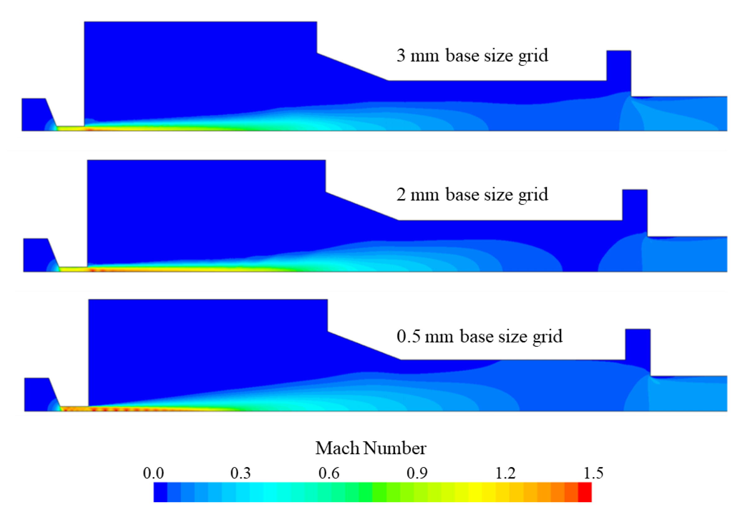
3. Computational Methods

The supersonic jet was modeled using a 2D axisymmetric computational fluid dynamics solver. The modeled fluid domain begins in the small cylindrical region immediately upstream of the showerhead nozzle and ends downstream of the plenum past the filter, as shown in Figure 5, with component dimensions, as shown in Figure 2.
The two filters were modeled using porous baffle interfaces. The porous viscous resistance values used in the solver, whose unit is m/s, were derived by dividing Equation (1) by ρ and Equation (2) by ρ ν .
A steady-state solver was used, as supported by the quasi-steady nature of the jet. Evidence of this quasi-steady nature is abundantly available in the experimental results that follow; see, for example, the interval between 0.12 s and 0.24 s.
Simulations were performed using the commercially available code STAR-CCM+ version 2020.1. A coupled implicit solver was employed, utilizing the realizable k ε two-layer RANS turbulence closure [15]. The ideal gas equation of state and a transport equation for energy were also used.
The transport equation for turbulent kinetic energy (k) is given by:
( ρ k ) t + ( ρ k u i ) x i = x j μ + μ t σ k k x j + G k + G b ρ ε Y M + S k .
The transport equation for the turbulent dissipation rate ( ε ) is:
( ρ ε ) t + ( ρ ε u i ) x i = x j μ + μ t σ ε ε x j + ρ C 1 S ε ρ C 2 ε 2 k + ν ε + C 1 ε ε k G b + S ε .
The turbulent viscosity ( μ t ) is calculated using:
μ t = ρ C μ k , ε , S k 2 ε , where C μ = 1 A 0 + A s U * k / ε .
For detailed definitions of the terms and coefficients, please refer to Shih et al. [15]. A 2D polyhedral grid mostly made of hexagons is used for spatial discretization, with a thin near-wall prism layer sufficient to ensure y + < 1 at the wall. Mach number values for three different grid sizes are shown in Figure 6, which highlights how finer shockwaves appear with a smaller mesh base size. A grid base size of 0.5 mm was adopted in the present work.

4. Results

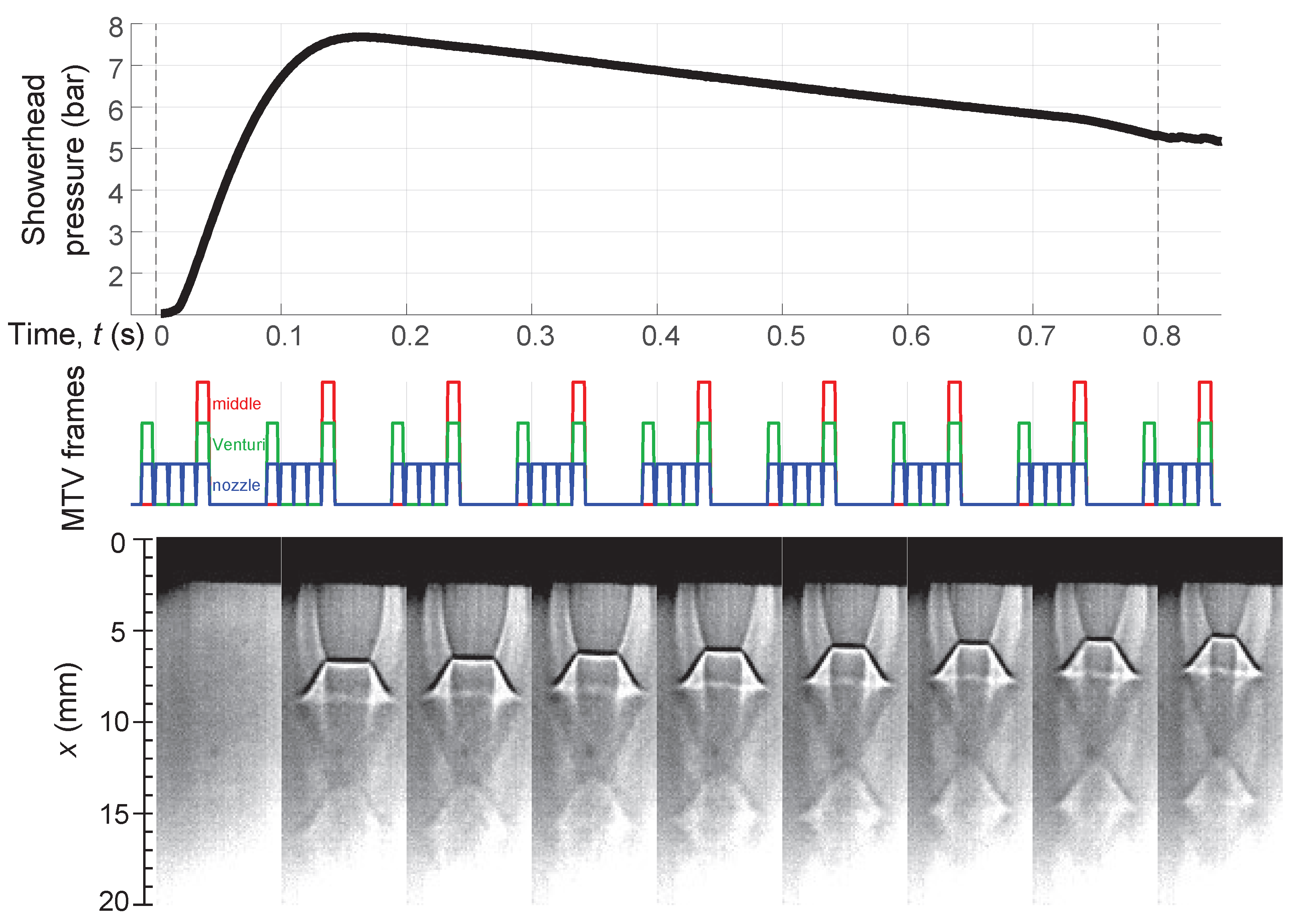
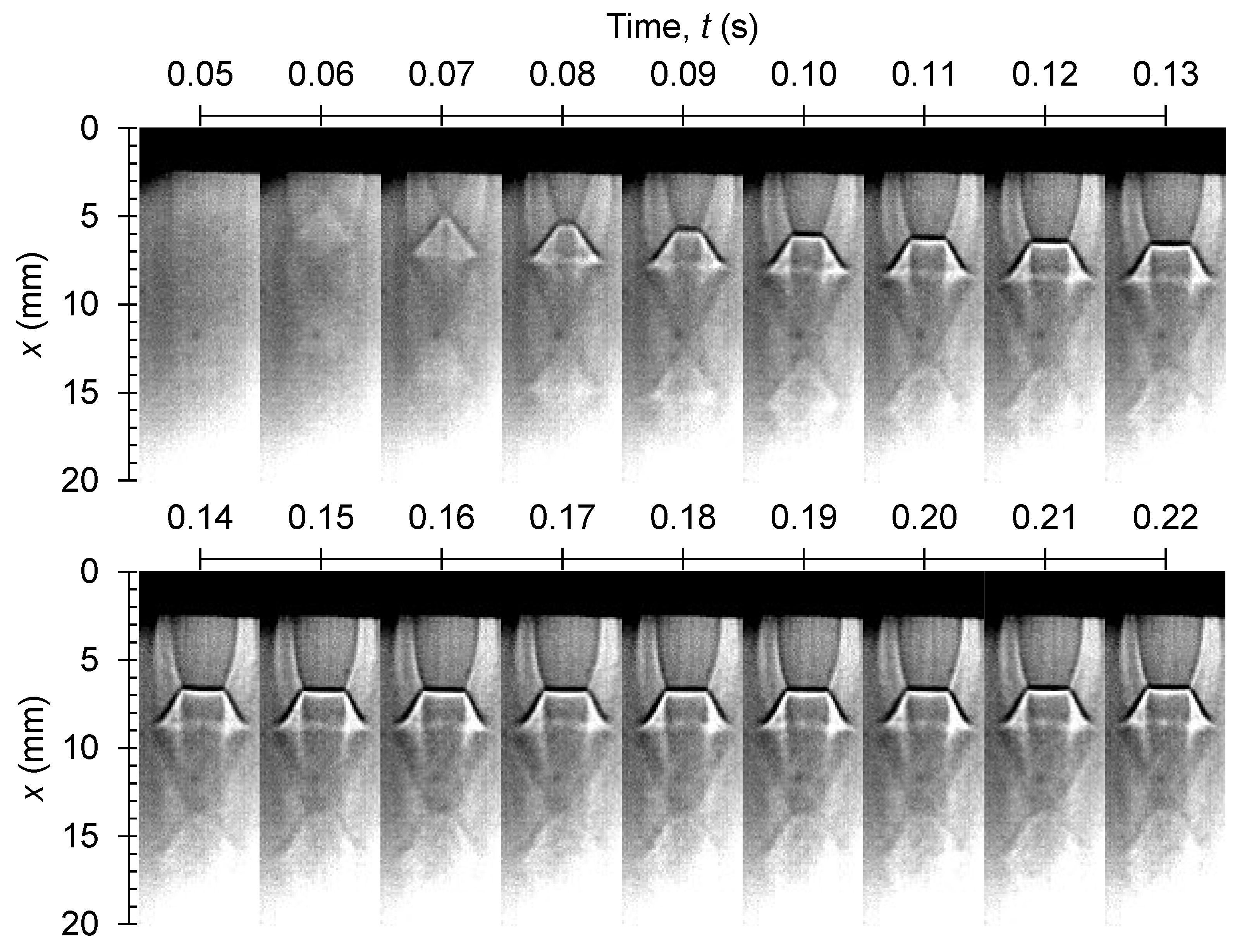
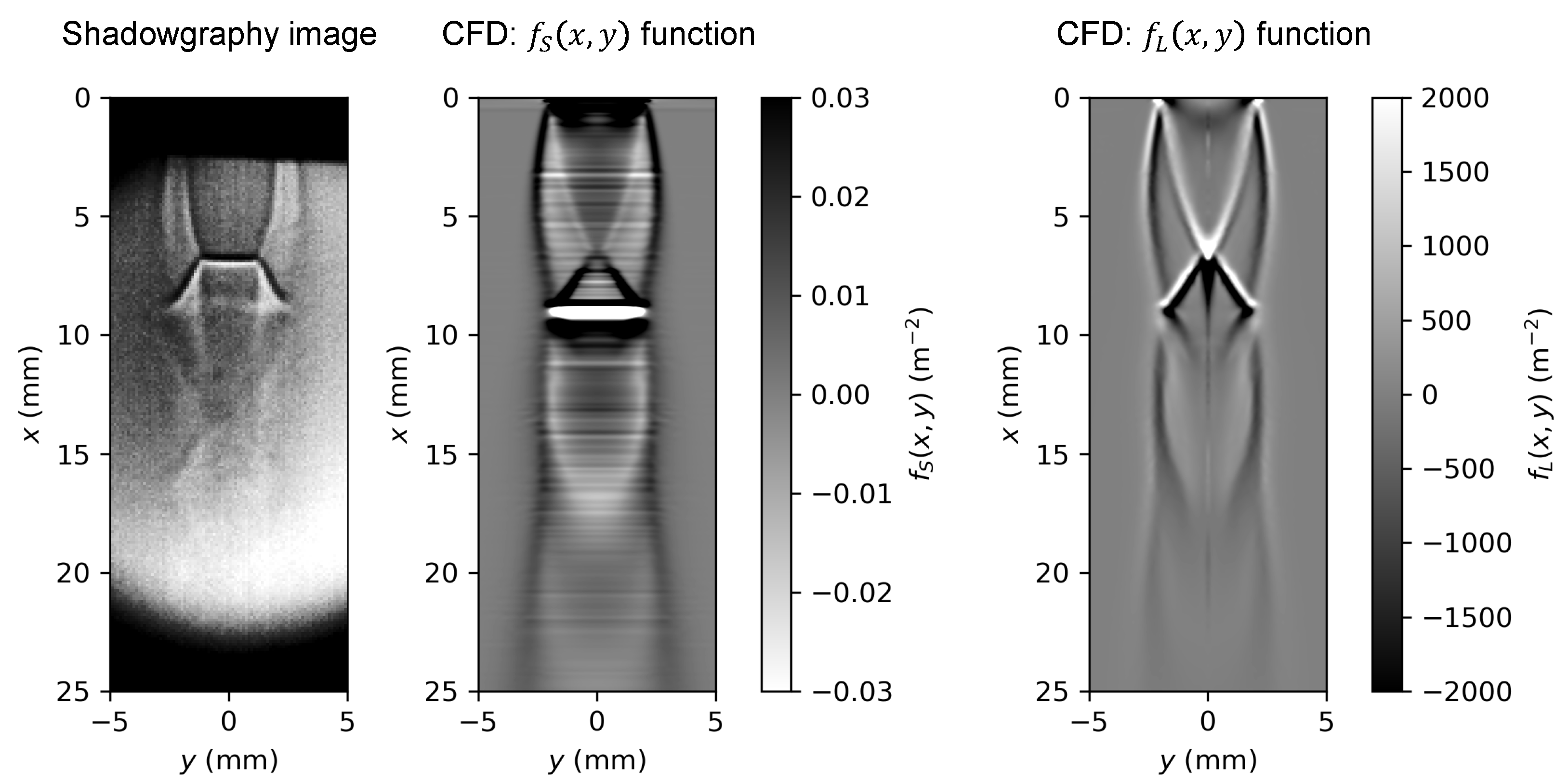
4.1. Shadowgraphy Results

Figure 4 shows the results from the shadowgraphy acquisitions during a 0.8 s pulse. Each frame is an average of 90 raw images (10 ms), and the figure displays one frame every 0.1 s from 0.05 to 0.85 ms after the gas pulse starts. The figure also shows the pressure measured in the showerhead volume upstream of the nozzle during the pulse (top). From the pressure time history, three regimes can be identified during one pulse. First, a transient is visible in the first 0.1 s as the pressure builds up in the showerhead. The pressure is then nearly steady between 0.12 and 0.24 s; this is the quasi-steady phase of the jet. Finally, the jet declines after 0.3 s as the pressure decreases exponentially.
At the entrance of the straight nozzle, a vena contracta develops, which allows the jet to transition to supersonic. Because the throat is not controlled, this results in an underexpanded supersonic jet, whose topology is recognizable in Figure 7. The three phases of the jet identified from the pressure history are confirmed by the shadowgraphy visualizations. Figure 7 presents additional shadowgraphy frames at the beginning of the pulse with shorter temporal increments. The bottom frames are for time 0.14 to 0.22 s and are nearly identical. There, the upstream pressure is high and the flow is highly underexpanded, leading to a sharp first Mach disk at x = 6.8 mm followed by additional Mach disks with reduced intensity and size. Typical features of an underexpanded jet are observed, including barrel shocks and reflected shocks. The pressure in the showerhead peaks at 97 psig (7.7 bar). As the upstream pressure decreases after 0.3 s, the width of the first Mach disk and its distance from the nozzle also decrease. We have developed an intensity-based single-pixel-accuracy algorithm to track the lateral extent (width) and X-location of the main Mach disk on the shadowgraphy frames. Figure 8 shows the discrete results as grey circles, along with further smoothing using a moving average. The three regimes are distinctly observable in the figure, with the first Mach disk reaching a maximum depth of 6.8 mm and a maximum width of 2.4 mm.
A comparison with CFD results is shown in Figure 9 for the quasi-steady phase of the jet. In the shadowgraphy images, the pixel intensity changes as the rays from the light source are deflected by local variations of the refractive index through the jet. Two quantities from the CFD results are displayed in the figure: the variable f S x , y that relates to the divergence of ray deflection and the simplified function f L ( x , y ) , which consists of the Laplacian of the refractive index (see definitions in Appendix A).
The CFD result predicts the approximate axial position of the first Mach disk within 0.5 mm, as well as its approximate size. The modeled Mach disk appears to be narrower compared to the experimental one, while the reflected shocks appear to have comparable sizes. The modeled f S x , y quantity in Figure 9 exhibits signs of numerical oscillation that can be addressed in future work by testing advanced numerical schemes such as those in the ROUND family [16,17].

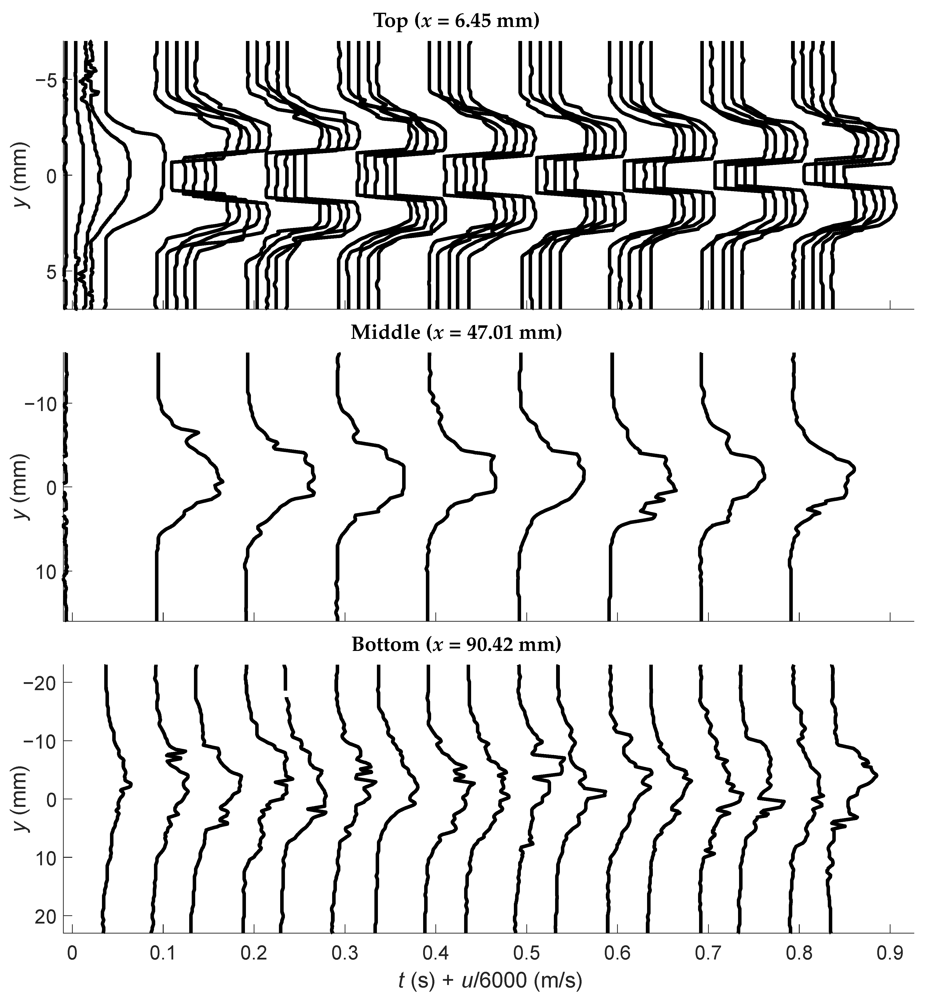
4.2. Molecular Tagging Velocimetry Results

Figure 10 shows the evolution of the instantaneous velocity profiles measured by MTV at the three locations. The MTV results confirm the findings from the shadowgraphy study (Figure 4 and Figure 7) as the signature of the Mach disk appears in the velocity profiles as early as 0.09 s after the gas pulse starts. The maximum measured velocity at the first MTV measurement station (a few millimeters below the nozzle) is 489 m/s (Mach 1.43); Figure 3 shows the raw MTV image with the deformed tagged line. This maximum speed decreases to 438 m/s (Mach 1.28) and 296 m/s (Mach 0.86) at the two other measurements downstream. The Reynolds number based on the 4 mm nozzle diameter is on the order of 10 6 , as calculated, for the sake of simplicity, using the measured 489 m/s velocity and ideal gas air properties inside the reservoir at 7.7 bar. The temporal evolution of the MTV profiles is divided into the three regimes identified above. Figure 11 highlights the three regimes by stacking multiple velocity profiles on a single plot. The transient leading to the existence of the Mach disk below the nozzle is shorter than 0.09 s after the gas pulse starts. A quasi-steady regime is then observed for t = 0.12 0.24 s, and the jet finally decreases after that: the Mach disk retracts laterally, and the peak flow velocity decreases. It should be noted that the first MTV measurement location is very close to the location of the main Mach disk in the quasi-steady regime; the subsonic center part of the velocity profile is characteristic of the subsonic flow in the jet core downstream of the Mach disk.
Figure 12 displays the validation of CFD versus MTV results in the quasi-steady regime. The quantities compared in that plot are streaklines. Streaklines indicate the destination position of fluid parcels that start along a given line in the domain after a given Δ t has elapsed; this is essentially a simulation of the MTV signal. For simplicity, those results are shown in Figure 12 with the dimension of velocity, representing the ratio between the distance from the starting line and Δ t . For the steady-state CFD results, well-converged streaklines are obtained by post-processing the velocity results using a time-marching Lagrangian algorithm and 100 iterations. The MTV velocity profiles plotted in the figure are the same as in Figure 11 (middle), obtained between 0.12 and 0.14 s. There are seven profiles for the top location ( x = 6.45 mm), one in the middle ( x = 47.01 mm), and three at the bottom location ( x = 90.42 mm).
General agreement in terms of trends and approximate magnitudes is observed between the CFD and MTV results at all three locations in which data are available. At the top line, both CFD and MTV show a dual-peaked streakline profile. MTV data show a low-velocity central feature a few millimeters wide that is not present in CFD results. This observation is consistent with the narrower Mach disk modeled by CFD as observed in Section 4.1.
Potential reasons justifying the narrower modeled Mach disk relative to the experiment may include the axisymmetric assumption applied to a complex three-dimensional geometry, limitations of the k ε turbulence model in the complex flow at hand, and steady-state modeling versus the inherently unsteady nature of shock structures.
Furthermore, while the 2D RANS method performs acceptably in the quasi-steady regime encountered in these tests, underexpanded jets that are not quasi-steady should be treated with unsteady models. In the domain of transient modeling, see, for example, the large-eddy simulation (LES) work by Vuorinen et al. [18] and Hamzehloo and Aleiferis [19].

5. Conclusions

MTV and shadowgraphy data were acquired for a filter pulse-jet cleaning underexpanded supersonic gas jet. Air was ejected at a pressure of up to 7.7 bar through a 4 mm diameter nozzle and directed towards a filtration system to mimic filter cleaning operation. A 489 m/s (Mach 1.43) pulse was measured by MTV 6.45 mm below the nozzle exit. The experimental data were compared to steady-state axisymmetric results from a coupled implicit realizable k ε CFD model.
A general similarity was observed between simulation and experiment. In both cases, the flow topology is identified as an underexpanded supersonic jet with a sharp first Mach disk 6-8 mm below the nozzle. The width of this first Mach disk is larger in experimental data compared to CFD, while reflected shocks appear to have comparable sizes. Besides this difference, streaklines from CFD are similar in trends and magnitudes to MTV data.

Author Contributions

Conceptualization, G.L., M.A.A., R.E.J., P.M.B. and C.R.M.; methodology, G.L., C.F., M.A.A. and P.M.B.; software, G.L., C.F. and V.P.; validation, G.L., C.F., M.A.A. and V.P.; formal analysis, G.L., C.F., M.A.A. and V.P.; investigation, G.L., C.F. and P.M.B.; resources, P.M.B.; writing—original draft preparation, G.L.; writing—review and editing, C.F., V.P. and P.M.B.; visualization, C.F.; supervision, R.E.J., P.M.B. and C.R.M.; project administration, R.E.J.; funding acquisition, R.E.J. All authors have read and agreed to the published version of the manuscript.

Funding

This research received financial support provided by the US Department of Energy Office of Environmental Management.

Institutional Review Board Statement

Not applicable.

Informed Consent Statement

Not applicable.

Data Availability Statement

The raw data supporting the conclusions of this article will be made available by the authors on request.

Acknowledgments

The authors are grateful to the Idaho Cleanup Project team working at the IWTU site for funding this project and providing inputs and recommendations. Members and consultants of that team include Craig Porter, Seabury Zolman, Stephen King, Robert Gross, James Fitch, Elizabeth Bush, Afshin Kazeminezhad, Gerald Zeininger, Allyson Ferry, and Rick Farnsworth. The authors also acknowledge invaluable support in portions of this project from Sean Lockard, who designed the test rig, and Daniel Hardy, who supported experimental acquisitions.

Conflicts of Interest

Authors Giancarlo Lenci, Ryan E. Jones and Chuck R. Marks were employed by the company Dominion Engineering. The remaining authors declare that the research was conducted in the absence of any commercial or financial relationships that could be construed as a potential conflict of interest.

Appendix A. Numerical Shadowgraphy Functions

CFD results have been converted in the functions shown in Figure 9 based on the following physical considerations that follow the equations in Settles [20] and applied to asymmetric cylindrical coordinates.
Features in shadowgraphy images are driven by changes in the fluid’s refractive index n. Such an index varies with the gas density ρ as described by the following linear relationship:
n 1 = k ρ ,
where k is the Gladstone–Dale coefficient (about 0.23 cm 3 / g for air at standard conditions). The angular ray deflection for light collimated in the z direction crossing a medium can be decomposed into x and y components and is obtained by integrating the respective gradients along the z direction:
ε x = 1 n 0 z n x d z ,
ε y = 1 n 0 z n y d z ,
where n 0 is the refractive index of the surrounding medium.
For an asymmetric geometry in cylindrical coordinates with x being the axial direction, y the radial direction, and z the direction of the collimated rays, Equations (A2) and (A3) correspond, respectively, to the following two equations:
ε x x , y = 2 n 0 y R n x x , y cot acos y R d y ,
ε y x , y = 2 R n 0 y R n y x , y y cot acos y R d y .
In shadowgraphy images, the pixel intensity shifts with changes (gradients) in this ray deflection. Therefore, the divergence of ray deflection,
f S x , y = ε x x , y x + ε y x , y y ,
is typically used to compare numerical results to shadowgrams. The variable f S x , y is used to convey the results in Figure 9. The figure also shows a simplified function that is often adopted in the literature, consisting of the Laplacian of the refractive index,
f L ( x , y ) = 2 n .
This function implies that the target has a thin planar geometry. Although this is an incorrect assumption, results using this variable are still provided for the reader’s benefit due to the ease of reproduction.

References

  1. Heidenreich, S. Chapter Eleven—Hot Gas Filters. In Progress in Filtration and Separation; Tarleton, S., Ed.; Academic Press: Oxford, UK, 2015; pp. 499–525. [Google Scholar]
  2. Ito, S. Pulse jet cleaning and internal flow in a large ceramic tube filter. In Gas Cleaning at High Temperatures; Clift, R., Seville, J.P.K., Eds.; Springer: Dordrecht, The Netherlands, 1993; pp. 266–279. [Google Scholar]
  3. Lo, L.M.; Hu, S.C.; Chen, D.R.; Pui, D.Y.H. Numerical study of pleated fabric cartridges during pulse-jet cleaning. Powder Technol. 2010, 198, 75–81. [Google Scholar] [CrossRef]
  4. Andersen, B.O.; Nielsen, N.F.; Walther, J.H. Numerical and experimental study of pulse-jet cleaning in fabric filters. Powder Technol. 2016, 291, 284–298. [Google Scholar] [CrossRef]
  5. Hsu, A.G.; Srinivasan, R.; Bowersox, R.D.; North, S.W. Two-component molecular tagging velocimetry utilizing NO fluorescence lifetime and NO2 photodissociation techniques in an underexpanded jet flowfield. Appl. Opt. 2009, 48, 4414–4423. [Google Scholar] [CrossRef] [PubMed]
  6. Inman, J.; Danehy, P.; Bathel, B.; Nowak, R. Laser-induced fluorescence velocity measurements in supersonic underexpanded impinging jets. In Proceedings of the 48th AIAA Aerospace Sciences Meeting Including the New Horizons Forum and Aerospace Exposition, Orlando, FL, USA, 4–7 January 2010. [Google Scholar]
  7. Parziale, N.J.; Smith, M.S.; Marineau, E.C. Krypton tagging velocimetry of an underexpanded jet. Appl. Opt. 2015, 54, 5094–5101. [Google Scholar] [CrossRef]
  8. Pitz, R.W.; Danehy, P.M. Molecular tagging velocimetry. In Optical Diagnostics for Reacting and Non-Reacting Flows: Theory and Practice; Steinberg, A., Roy, S., Eds.; AIAA: Reston, VA, USA, 2023; pp. 539–588. [Google Scholar]
  9. Stewart, J.R. CFD modelling of underexpanded hydrogen jets exiting rectangular shaped openings. Process Saf. Environ. Prot. 2020, 139, 283–296. [Google Scholar] [CrossRef]
  10. Hata, M.; Kanaoka, C.; Furuuchi, M.; Inagaki, T. Analysis of Pulse-Jet Cleaning of Dust Cake from Ceramic Filter Element; Technical Report; Kanazawa University: Kanazawa, Japan, 2002. [Google Scholar]
  11. Laux, S.B.H.U.; Giernoth, B.; Bulak, H.; Renz, U. Aspects of pulse-jet cleaning of ceramic filter elements. In Gas Cleaning at High Temperatures; Clift, R., Seville, J.P.K., Eds.; Springer: Dordrecht, The Netherlands, 1993; pp. 203–224. [Google Scholar]
  12. Morris, K.; Cursley, C.J.; Allen, R.W.K. The role of venturis in pulse-jet filters. Filtr. Sep. 1991, 28, 33–36. [Google Scholar] [CrossRef]
  13. Liu, X.; Shen, H. Effect of venturi structures on the cleaning performance of a pulse jet baghouse. Appl. Sci. 2019, 9, 3687. [Google Scholar] [CrossRef]
  14. André, M.A.; Burns, R.A.; Danehy, P.M.; Cadell, S.R.; Woods, B.G.; Bardet, P.M. Development and application of molecular tagging velocimetry for gas flows in thermal hydraulics. Nucl. Technol. 2019, 205, 262–271. [Google Scholar] [CrossRef]
  15. Shih, T.-H.; Liou, W.W.; Shabbir, A.; Yang, Z.; Zhu, J. A new k-ϵ eddy viscosity model for high Reynolds number turbulent flows. Comput. Fluids 2016, 24, 227–238. [Google Scholar] [CrossRef]
  16. Deng, X. A unified framework for non-linear reconstruction schemes in a compact stencil. Part 1: Beyond second order. J. Comput. Phys. 2023, 481, 112052. [Google Scholar] [CrossRef]
  17. Deng, X. A new open-source library based on novel high-resolution structure-preserving convection schemes. J. Comput. Sci. 2023, 74, 102150. [Google Scholar] [CrossRef]
  18. Vuorinen, V.; Yu, J.; Tirunagari, S.; Kaario, O.; Larmi, M.; Duwig, C.; Boersma, B.J. Large-eddy simulation of highly underexpanded transient gas jets. Phys. Fluids 2013, 25, 016101. [Google Scholar] [CrossRef]
  19. Hamzehloo, A.; Aleiferis, P.G. Numerical modelling of transient under-expanded jets under different ambient thermodynamic conditions with adaptive mesh refinement. Int. J. Heat Fluid Flow 2016, 61, 711–729. [Google Scholar] [CrossRef]
  20. Settles, G.S. Basic Concepts. In Schlieren and Shadowgraph Techniques: Visualizing Phenomena in Transparent Media; Springer: Berlin/Heidelberg, Germany, 2001; pp. 25–38. [Google Scholar]
Figure 1. Experimental setup and main components.
Applsci 15 05764 g001
Figure 2. Key dimensions (in mm) of flow boundaries in the test rig.
Applsci 15 05764 g002
Figure 3. Overview of the MTV and shadowgraphy setup.
Applsci 15 05764 g003
Figure 4. (Top figure): measured showerhead pressure vs. time during the discharge transient. (Middle figure): time sequence of the phase-averaged MTV frames recorded at three different heights downstream of the nozzle at 10 Hz frequency during the 0.8 s gas pulse. One, two, and five phases are acquired at the (top) (nozzle), (middle,bottom) (Venturi) measurement stations, respectively. (Lower figure): shadowgraphy images averaged over 10 ms show the evolution of the Mach disk below the nozzle from t = 0.05 to 0.85 s.
Applsci 15 05764 g004
Figure 5. CFD simulation domain visually compressed in the axial direction.
Applsci 15 05764 g005
Figure 6. Mach number in the portion of the simulation domain closest to the nozzle for three different grid sizes.
Applsci 15 05764 g006
Figure 7. Time evolution of shadowgraphy results in 10 ms increments from time 0.05 to 0.22 s; each frame is an average of 90 raw images captured during the 10 ms time window. The figure shows the evolution and quasi-steady nature of the Mach disks below the nozzle.
Applsci 15 05764 g007
Figure 8. Temporal evolution of the lateral extent (width) and X-location of the main Mach disk. The grey circles are obtained at single-pixel accuracy from the shadowgraphy images and the solid dark line smooths the data using a moving average.
Applsci 15 05764 g008
Figure 9. Comparison between shadowgraphy (left) and CFD density field (center, right) in a vertical slice of the flow domain. The figure highlights similarities and differences between the experimental and numerical fields for the Mach disk structure.
Applsci 15 05764 g009
Figure 10. Evolution of the instantaneous velocity profiles and their evolution in time measured by MTV at the three vertical locations, one for each plot. The figure shows the quasi-steady nature of the flow structures.
Applsci 15 05764 g010
Figure 11. Temporal evolution of the MTV profiles at three different heights downstream of the nozzle (top station at x = 6.45 mm, middle station at x = 47.01 mm, and bottom station at x = 90.42 mm). The three plots shown divide the gas pulse history into three regimes.
Applsci 15 05764 g011
Figure 12. Comparison between MTV (solid lines colored as in Figure 4) and CFD (filled circles) streaklines at three vertical elevations downstream of the nozzle (top station at x = 6.45 mm, middle station at x = 47.01 mm, and bottom station at x = 90.42 mm). The MTV velocity profiles are the same as in Figure 11 in the quasi-steady regime.
Applsci 15 05764 g012
Disclaimer/Publisher’s Note: The statements, opinions and data contained in all publications are solely those of the individual author(s) and contributor(s) and not of MDPI and/or the editor(s). MDPI and/or the editor(s) disclaim responsibility for any injury to people or property resulting from any ideas, methods, instructions or products referred to in the content.

